Epileptic Seizure Data Classification Using RBAs and Linear SVM

Published by Oriental Scientific Publishing Company © 2019

This is an Open Access article licensed under a Creative Commons license: Attribution 4.0 International (CC-BY).

Epileptic Seizure Data Classification Using

RBAs and Linear SVM

Alpika Tripathi

_{, Geetika Srivastava}

_{, K.K. Singh}

_{and P.K. Maurya}

1_{Department of Computer Science and Engineering, ASET, Amity University, Lucknow, India,} 2_{Department of Physics and Electronics, Dr. RML Avadh University, Faizabad, India.}

3_{Department of E&CE, ASET, Amity University, Lucknow, India.} 4_{Department of Neurology, RML Institute of Medical Sciences, Lucknow,India.}

*Corresponding autho E-mail: [email protected] http://dx.doi.org/10.13005/bpj/1674

(Received: 15 April 2019; accepted: 18 June 2019)

The objective of this paper is to make a distinction between EEG data of normal and epileptic subjects. Methods: The dataset is taken from 20-30 years healthy male/female subjects from EEG lab of Dept. of Neurology, Dr. RML Institute of Medical Sciences, Lucknow (India). The feature extraction has been done using the Hilbert Huang Transform (HHT) method. The experimental EEG signals have been decomposed till 5th level of Intrinsic Mode Function (IMF) followed by calculation of high order statistical values of each IMF. Relief algorithm (RBAs) is used for feature selection and classification is performed using Linear Support Vector Machine (Linear SVM). Findings: This paper gives an independent approach of classifying Epileptic EEG data with reduced computational cost and high accuracy. Our classification result shows sensitivity, specificity, selectiv ity and accuracy of 96.4%, 79.16%, 84.3% and 88.5% respectively. Application: The proposed method has been analyzed to be very effective in accurate classification of epileptic EEG data with high sensitivity.

Keywords: Epilepsy, EEG, Hilbert Huang Transform (HHT), Relief-based feature selection algorithms (RBAs), Linear Support Vector Machine (SVM).

E

PILEPSY

is a physical condition

that occurs in the brain and affects the nervous

system. According to the 2009 report by the World

Health Organization around 70 million people

worldwide have epilepsy

_{. Around 90% of this}

population lives in developing countries, and about

three fourths of them do not have access to the

necessary treatment. Epilepsy is defined by two

or more such unprovoked seizures

_{. The seizures}

are commonly defined as abnormal electrical and

chemical activities in the brain. Like many other

neurological disorders, epilepsy can be assessed by

the electroencephalogram (EEG). The EEG signal

is highly non-linear and non-stationary in nature,

and hence, it is difficult to characterize and interpret

it using conventional frequency domain analysis

_.

EEG is recording of the electrical

activity of the brain from the scalp. The recorded

waveforms reflect the cortical electrical activity

and helps in identification of brain conditions. The

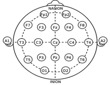
The system is based on the relationship

between the location of an electrode and the

underlying area of outer layer of the brain. The

number ‘10’ & ‘20’ refer to the distance between

adjacent electrode to be either 10% or 20% of the

total front-back or right-left distance of the scalp .

The electrode placement is shown in Fig.1.

In this paper authors have given a method

for classification of epileptic and normal EEG data.

The proposed method uses a combination of Hilbert

Huang Transform (HHT) for features extraction,

RBAs for feature selection and Linear SVM based

classification of neural network modeling.

Hilbert-Huang Transform is a time

frequency technique consisting of two parts, the

Empirical Mode Decomposition (EMD), and

the Hilbert Spectral Analysis (HSA)

_{. EMD}

decomposes an EEG signal into a finite set of

band-limited signals termed intrinsic mode functions

(IMFs), which are oscillatory components of input

data. In the first step the mean frequency (MF)

for each IMF has been computed using

Fourier-Bessel expansion

_{. The IMF oscillates in a narrow}

frequency band which is a reflection of

quasi-periodicity and nonlinearity. The non-constant

frequency means non-stationary. MF measure of

the IMFs has been used as one of the features to

differentiate between healthy and epileptic EEG

signals. In the second part, the Hilbert transform

is applied to the IMF, yielding a time-frequency

representation (Hilbert spectrum) for each IMF

_.

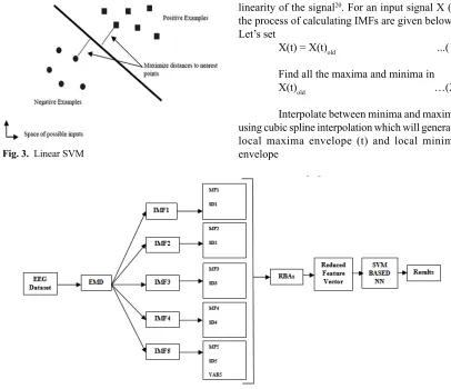
For feature selection authors have

used Relief algorithm

_{. Relief is an algorithm}

in which a filter-method approach is used for

feature selection that is notably sensitive to

feature interactions. It was originally designed

for application to binary classification problems

with discrete or numerical features. Relief was

also described as generalizable to polynomial

classification by decomposition into a number of

binary problems.

Relief calculates a feature score for each

feature which can then be applied to rank and

select top scoring features for feature reduction.

Alternatively, these scores may be applied as

feature weights to guide downstream modeling.

Relief feature scoring is based on the identification

of feature value differences between nearest

neighbor instance pairs. If a feature value difference

is observed in a neighboring instance pair with the

same class (a ‘hit’), the feature score decreases.

Alternatively, if a feature value difference is

observed in a neighboring instance pair with

different class values (a ‘miss’), the feature score

increases shown in Fig.2.

The Support Vector Machine (SVM) is

a popular classifier that can handle linear as well

as non-linear class boundaries with the help of

kernel functions

_{. In this paper authors have used}

Linear SVM for data classification. The SVM tries

to identify the maximum-margin hyper plane that

separates the different classes. However, if the data

cannot be linearly separated, non-linear kernel

functions are used to transform the feature space,

allowing a maximum-margin hyper plane to be

established

_.

HHT based feature extraction

The Hilbert–Huang transform (HHT) is

an empirical data-analysis method. Its basis of

expansion is adaptive, so it produces physically

meaningful representations of data from nonlinear

and non-stationary processes

_{. Traditional}

data-analysis methods are all based on linear and

stationary assumptions like Fourier transformation

makes assumption of the signal period which

creates spectral leakage. As is well known, the

natural physical processes are mostly nonlinear

and non-stationary like EEG signals from brain,

yet the conventional data analysis methods provide

very limited options for examining data from

such processes. The available methods are either

for linear but non-stationary, or nonlinear but

stationary and statistically deterministic processes.

It is known that frequency of sinusoidal

waveform is a well defined quantity. However,

in practice, signals are not purely sinusoidal or

stationary. Thus representing such non stationary

signals as combination of different sinusoidal

components will be a compromise with the accurate

assessment of an event. For such signal the term

frequency loses its effectiveness and a need for a

parameter which accounts for the varying nature

of the phenomena arises.

This gives rise to an idea of instantaneous

frequency (IF) – which means the signal is either

composed of a single frequency or a narrow band

of frequencies. For each component instantaneous

frequency can be defined.

HHT was motivated by the need to

describe nonlinear distorted waves in detail, along

with the variations of these signals that naturally

occur in non-stationary processes.

The empirical mode decomposition

method is necessary to deal with data from

non-stationary and nonlinear processes

_.

EMD decomposes signal X (t) into a number of

oscillatory component which is known as intrinsic

mode function through a shifting process. Each

IMF has its own distinct time scale. Furthermore

EMD does not consider the stationary and the

linearity of the signal

_{. For an input signal X (t)}

the process of calculating IMFs are given below:

Let’s set

X(t) = X(t)

...(1)

Find all the maxima and minima in

X(t)

…(2)

Interpolate between minima and maxima

using cubic spline interpolation which will generate

local maxima envelope (t) and local minima

envelope

Fig. 3. Linear SVM

Fig. 5. IMFs of Normal EEG Signal Fig. 6. IMFs of Epileptic EEG Signal

el(t)

...(3)

Calculate the mean of envelopes

emean = ((t) + el (t))/2

...(4)

Now subtract emean from X(t)

we will

get X(t)

as,

X(t)

= X(t)

- emean

...(5)

Now set

X(t)

= X(t)

...(6)

Repeat the process (2 to 4) until standard deviation

SD = (

S |

X(t)

–X(t)

|

_/

_S

_X(t)

) <

a

...(7)

Where

a

is value that between 0.2-0.3

The first IMF is defined as IMF1 = X(t)

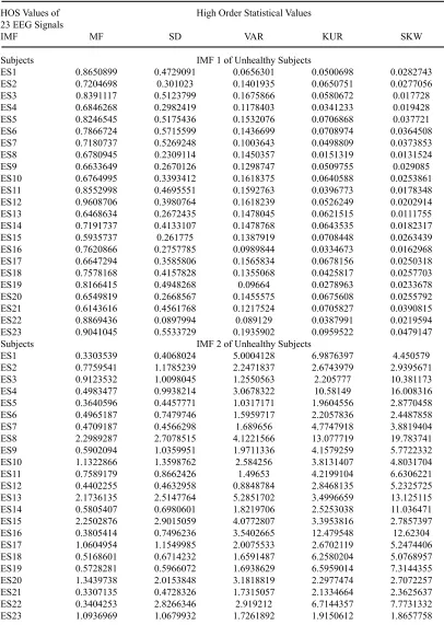
Table 1 . High Order Statistical Values of 29 EEG signal of Normal Subjects upto 5th _IMF

HOS Values of High Order Statistical Values

29 EEG Signals

IMF MF SD VAR KUR SKW

Subjects IMF 1 of Healthy Subjects

NS1 0.794014 0.194748 0.0808656 0.0574944 0.0275939

NS2 0.7134649 0.3835633 0.1539171 0.0777196 0.0382288

NS3 0.7120425 0.392048 0.125765 0.0633654 0.0277442

NS4 0.6561924 0.3911876 0.1600673 0.0619577 0.0186501

NS5 0.7923439 0.39687 0.1419385 0.0608046 0.0248904

NS6 0.69531 0.3801633 0.1490987 0.0560318 0.0249986

NS7 0.6191468 0.3552116 0.1217889 0.0628417 0.0204335

NS8 0.6190132 0.2576959 0.1470799 0.0867544 0.0133281

NS9 0.7279635 0.3972242 0.1589645 0.0708214 0.0291047

NS10 0.6938438 0.3249872 0.1626327 0.0611141 0.0319724

NS11 0.6037114 0.2716271 0.1364642 0.0631772 0.0158963

NS12 0.5959096 0.2387053 0.1123194 0.0494584 0.0204792 NS13 0.7039527 0.3296545 0.1480881 0.0748475 0.0269281 NS14 0.6844529 0.4312466 0.165582 0.0781406 0.0422987 NS15 0.7843782 0.4633051 0.1519389 0.0567255 0.0207948 NS16 0.7207146 0.356144 0.1542686 0.0732491 0.023715 NS17 0.7776593 0.4194125 0.157747 0.0816223 0.0360981 NS18 0.7018462 0.4333557 0.1727692 0.0736394 0.0344944 NS19 0.7561062 0.3031047 0.1599127 0.0667163 0.0298385 NS20 0.5615601 0.2440335 0.1393101 0.0625563 0.0232113 NS21 1.0151271 0.5419102 0.2060411 0.1060046 0.0350871 NS22 0.7082527 0.4058785 0.1250664 0.061215 0.0242943

NS23 0.58942 0.2640501 0.1342691 0.0745797 0.0292519

NS24 0.6863921 0.2591281 0.1569117 0.0679083 0.0330215 NS25 0.6579692 0.3820743 0.1577376 0.0544039 0.0247068 NS27 0.6185096 0.3248713 0.1347292 0.0557921 0.0208321 NS28 0.7167416 0.2263721 0.1505363 0.0735477 0.0337342 NS29 0.4230327 0.3507278 0.1417878 0.0668265 0.026326

Subjects IMF 2 of Healthy Subjects

NS1 1.3671451 2.8716697 6.5527059 9.3498067 8.6381729

NS2 1.1840138 1.3916471 2.8017808 2.4379485 2.2303501

NS3 0.843453 0.9167091 2.4823977 3.5295424 3.3642967

NS4 0.8421751 0.9637028 2.2007558 2.8008546 5.2072605

NS5 0.5406368 0.9089775 2.0956593 4.9641066 2.7387957

NS6 0.6736103 0.8451676 2.1182751 3.4507008 3.1589237

NS7 0.9872215 1.0550772 2.5285452 2.9370106 5.9665401

NS8 4.5190525 6.5279076 9.970391 5.4465119 20.088837

NS9 0.5998085 0.8185307 1.6512623 2.3169359 3.1302619

NS10 0.8223158 1.0699668 1.8031497 2.367291 2.5566929 NS11 1.0965751 1.460845 2.553014 2.7946504 5.9919763 NS12 1.1829003 1.7480142 3.5795746 4.8171016 4.7400878 NS13 1.0971638 1.4864917 2.6012838 2.1556349 2.5493749 NS14 0.4312608 0.5038683 0.9079241 1.3058499 1.4082351 NS15 1.5704348 1.487021 2.6870926 7.916428 14.940614 NS16 0.8077475 1.0170576 2.5210509 2.3879847 2.7999426 NS17 0.4905736 0.7537514 1.8861905 1.9574766 1.9970076 NS18 0.7166195 1.0073588 2.0143632 2.1873461 2.7866116

NS19 0.680081 1.1124491 1.9422344 2.3306878 3.7269487

NS21 3.0527935 3.1810749 2.9614952 2.9901266 2.0240628 NS22 0.6201656 0.6909153 2.2992595 3.5640906 3.9328668 NS23 2.1344174 2.6372075 4.8936201 3.6146932 3.2462856 NS24 0.5554465 1.3915533 2.3443719 2.6064464 1.9867625 NS25 1.0111484 1.1234713 2.0467199 3.0696111 2.481803 NS27 1.1047307 1.2129053 2.3732381 3.3731465 5.2515313 NS28 0.6727835 1.6808005 3.1633969 3.2929552 2.621261 NS29 0.5791149 0.5605072 1.4387479 1.9286429 3.2353766

Subjects IMF 3 of Healthy Subjects

NS1 1.8690857 8.246487 42.937955 87.418885 74.618031

NS2 1.4018887 1.9366815 7.8499754 5.9435931 4.9744615

NS3 0.7114129 0.8403556 6.1622985 12.45767 11.318492

NS4 0.7092588 0.928723 4.8433261 7.8447862 27.115562

NS5 0.2922881 0.8262401 4.3917878 24.642354 7.5010021

NS6 0.4537508 0.7143082 4.4870895 11.907336 9.978799

NS7 0.9746063 1.1131878 6.3935406 8.6260312 35.5996

NS8 20.421835 42.613577 99.408696 29.664492 403.56139

NS9 0.3597703 0.6699926 2.7266671 5.3681922 9.7985398

NS10 0.6762032 1.144829 3.251349 5.6040665 6.5366786

NS11 1.2024769 2.1340681 6.5178805 7.8100709 35.90378

NS12 1.399253 3.0555538 12.813354 23.204467 22.468433

NS13 1.2037684 2.2096577 6.7666774 4.6467616 6.4993125 NS14 0.1859859 0.2538833 0.8243261 1.705244 1.9831261 NS15 2.4662655 2.2112313 7.2204666 62.669832 223.22196

NS16 0.652456 1.0344061 6.3556978 5.7024708 7.8396784

NS17 0.2406624 0.5681411 3.5577147 3.8317147 3.9880392 NS18 0.5135434 1.0147717 4.0576589 4.7844829 7.7652043 NS19 0.4625101 1.237543 3.7722746 5.4321057 13.890147 NS20 9.5021525 16.882242 31.493774 21.548588 15.322308 NS21 9.3195484 10.119238 8.770454 8.940857 4.0968302 NS22 0.3846054 0.477364 5.2865944 12.702742 15.467441 NS23 4.5557378 6.9548636 23.947518 13.066007 10.53837 NS24 0.3085208 1.9364205 5.4960795 6.7935628 3.9472251 NS25 1.0224211 1.2621877 4.1890623 9.4225121 6.1593459

NS27 1.22043 1.4711394 5.6322589 11.378117 27.578581

NS28 0.4526377 2.8250902 10.00708 10.843554 6.871009 NS29 0.3353741 0.3141683 2.0699954 3.7196636 10.467662

Subjects IMF 4 of Healthy Subjects

NS1 26.1211 173.58881 105.7402 86.502577 14.866722

NS2 4.5384237 5.8235914 3.3288413 3.9677612 3.7352665

NS3 4.4268523 6.0777767 6.4834451 4.3057737 4.129212

NS4 13.246323 6.5958737 3.7837047 3.3066044 4.5568696

NS5 5.8715379 9.3080921 4.438701 2.8511137 3.3463041

NS6 4.7410993 5.602009 3.5239203 3.5818778 3.7913422

NS7 5.019083 4.3211797 7.0526305 3.8742989 6.3995483

NS8 12.323221 26.213322 6.9748686 5.203992 14.349722

NS9 5.2998872 8.1148395 4.0907434 3.5577341 2.7479037

NS10 5.5523941 15.273256 3.2721178 4.860471 3.6195343

NS11 5.1316229 7.6528964 3.4040442 3.4681068 11.761679

NS18 7.3879998 3.6279616 3.2416907 4.0381763 12.696512 NS19 124.96265 7.2477353 3.3237369 3.8798556 5.3328726 NS20 4.8953379 6.7082148 3.0854336 4.6323791 5.6055095 NS21 19.483011 18.089693 4.9513198 4.9412625 2.9780993 NS22 18.376056 6.0605848 5.1925368 7.9395411 9.4866847 NS23 4.3802035 6.3862992 3.1073743 2.9512085 8.2121815 NS24 5.8519008 7.5350298 3.1145678 3.5716336 4.0131338 NS25 4.8353898 4.4480728 3.2057832 6.4106097 4.777637 NS27 6.9280576 6.504447 5.4986645 7.9219861 13.547343 NS28 81.381915 12.772316 3.7331439 3.2206681 3.218636 NS29 859.94158 22.498134 4.7187115 4.8681671 4.070564

Subjects IMF 5 of Healthy Subjects

NS1 0.9368617 2.2400095 1.8788759 -4.6346204 -0.4742972

NS2 -0.0641331 0.02556 0.0213764 -0.1746376 -0.1316439

NS3 -0.0329525 -0.0372348 -0.170347 0.03744 -0.2469791

NS4 0.0760672 -0.0646503 0.078916 -0.0567486 0.265975

NS5 0.1335422 -0.0651292 -0.0394491 -0.1116554 -0.5056581

NS6 -0.0182776 -0.1920655 0.0125293 -0.0639116 0.2236741

NS7 0.0518529 0.0462345 0.2674941 0.0297923 -0.7641902

NS8 0.0091883 -0.2378462 0.0179487 0.0271938 1.0651003

NS9 -0.0182481 -0.0174901 0.0300339 0.0872897 -0.0599968

NS10 -0.0801845 0.6202513 -0.0045994 0.2976808 -0.0249067

NS11 -0.039921 0.3110126 0.086128 -0.0891201 -0.345381

NS12 1.2827003 -0.0110624 -0.0726262 0.0017892 -0.6870894

NS13 0.0069424 -0.0484375 0.0417263 -0.1836737 0.3871868

NS14 -0.6105902 1.2346839 0.1682674 0.0953418 -0.0021122

NS15 -0.1261543 -0.4746706 -0.3580666 0.2197198 -0.0952142

NS16 0.0352776 0.2623286 0.0164817 0.1063452 -0.2706383 NS17 -0.0915483 0.0119703 -0.0373728 0.0496959 0.2590188

NS18 0.1835534 0.0202854 -0.0084826 0.0108377 0.9936275

NS19 4.2085615 0.0127075 -0.059354 -0.2144468 -0.2042717

NS20 -0.0086416 -0.0772461 -0.0441348 -0.0245628 0.4144225

NS21 0.1078166 0.2286214 0.0188273 0.0214265 0.000411 NS22 -0.6105868 -0.1642786 0.0458767 0.8285085 -0.2906335 NS23 0.0155542 0.1616218 0.0071227 -0.0232878 -1.1183538

NS24 -0.0677949 -0.0092523 0.0438202 -0.0172195 -0.2904886

NS25 -0.0088769 0.0240307 -0.0392672 0.3934843 0.5874376

NS27 -0.0855313 -0.0039345 -0.1527337 0.2219079 -0.7106446

NS28 -0.3867619 -0.1214849 -0.0287683 -0.0250265 -0.1046807

NS29 24.095343 -0.4350748 0.0042242 0.0465327 -0.1108155

subtracting IMF1 from X(t) we will get residual

signal R(t) which can be expressed as ,

R(t) = X(t) – IMF1.

After acquiring R(t) we put it in the same

process above to get new IMF which means each

IMF will have different frequencies against time.

So the original signal can be rewritten as

Hilbert Huang Transform (HHT) is a very

new and powerful tool for analyzing data from

non-stationary and nonlinear processing realm

and capable of filtering data based on empirical

mode decomposition (EMD). The EMD is based

on the sequential extraction of energy associated

with various intrinsic time scales of the signal;

therefore total sum of the intrinsic mode functions

(IMFs) matches the signal very well and ensures

completeness.

Table 2. High Order Statistical Values of 23 EEG signal of Epileptic Subjects upto 5th _IMF

HOS Values of High Order Statistical Values

23 EEG Signals

IMF MF SD VAR KUR SKW

Subjects IMF 1 of Unhealthy Subjects

ES1 0.8650899 0.4729091 0.0656301 0.0500698 0.0282743

ES2 0.7204698 0.301023 0.1401935 0.0650751 0.0277056

ES3 0.8391117 0.5123799 0.1675866 0.0580672 0.017728

ES4 0.6846268 0.2982419 0.1178403 0.0341233 0.019428

ES5 0.8246545 0.5175436 0.1532076 0.0706868 0.037721

ES6 0.7866724 0.5715599 0.1436699 0.0708974 0.0364508

ES7 0.7180737 0.5269248 0.1003643 0.0498809 0.0373853

ES8 0.6780945 0.2309114 0.1450357 0.0151319 0.0131524

ES9 0.6633649 0.2670126 0.1298747 0.0509755 0.029085

ES10 0.6764995 0.3393412 0.1618375 0.0640588 0.0253861

ES11 0.8552998 0.4695551 0.1592763 0.0396773 0.0178348

ES12 0.9608706 0.3980764 0.1618239 0.0526249 0.0202914

ES13 0.6468634 0.2672435 0.1478045 0.0621515 0.0111755

ES14 0.7191737 0.4133107 0.1478768 0.0643535 0.0182317

ES15 0.5935737 0.261775 0.1387919 0.0708448 0.0263439

ES16 0.7620866 0.2757785 0.0989844 0.0334673 0.0162968

ES17 0.6647294 0.3585806 0.1565834 0.0678156 0.0250318

ES18 0.7578168 0.4157828 0.1355068 0.0425817 0.0257703

ES19 0.8166415 0.4948268 0.09664 0.0278963 0.0233678

ES20 0.6549819 0.2668567 0.1455575 0.0675608 0.0255792

ES21 0.6143616 0.4561768 0.1217524 0.0705827 0.0390815

ES22 0.8869436 0.0897994 0.089129 0.0387991 0.0219594

ES23 0.9041045 0.5533729 0.1935902 0.0959522 0.0479147

Subjects IMF 2 of Unhealthy Subjects

ES1 0.3303539 0.4068024 5.0004128 6.9876397 4.450579

ES2 0.7759541 1.1785239 2.2471837 2.6743979 2.9395671

ES3 0.9123532 1.0098045 1.2550563 2.205777 10.381173

ES4 0.4983477 0.9938214 3.0678322 10.58149 16.008316

ES5 0.3640596 0.4457771 1.0317171 1.9604556 2.8770458

ES6 0.4965187 0.7479746 1.5959717 2.2057836 2.4487858

ES7 0.4709187 0.4566298 1.689656 4.7747918 3.8819404

ES8 2.2989287 2.7078515 4.1221566 13.077719 19.783741

ES9 0.5902094 1.0359951 1.9711336 4.1579259 5.7722332

ES10 1.1322866 1.3598762 2.584256 3.8131407 4.8031704

ES11 0.7589179 0.8662426 1.49653 4.2199104 6.6306221

ES12 0.4402255 0.4632958 0.8848784 2.8468135 5.2325725

ES13 2.1736135 2.5147764 5.2851702 3.4996659 13.125115

ES14 0.5805407 0.6980601 1.8219706 2.5253038 11.036471

ES15 2.2502876 2.9015059 4.0772807 3.3953816 2.7857397

ES16 0.3805414 0.7496236 3.5402665 12.479548 12.62304

ES17 1.0604954 1.1549985 2.0075533 2.6702119 5.2474406

ES18 0.5168601 0.6714232 1.6591487 6.2580204 5.0768957

ES19 0.5728281 0.5966072 1.6938629 6.5959014 7.3144355

ES20 1.3439738 2.0153848 3.1818819 2.2977474 2.7072257

ES21 0.3307135 0.4728326 1.7315057 2.1334664 2.3625637

ES22 0.3404253 2.8266346 2.919212 6.7144357 7.7731332

Subjects IMF 3 of Unhealthy Subjects

ES1 0.1091337 0.1654882 25.004129 48.827109 19.807653

ES2 0.6021047 1.3889186 5.0498348 7.1524041 8.6410547

ES3 0.8323884 1.0197052 1.5751663 4.8654523 107.76876

ES4 0.2483504 0.987681 9.4115946 111.96793 256.26619

ES5 0.1325394 0.1987172 1.0644402 3.8433861 8.2773925

ES6 0.2465308 0.5594661 2.5471256 4.8654812 5.9965518

ES7 0.2217644 0.2085108 2.8549373 22.798637 15.069461

ES8 5.2850734 7.3324599 16.992175 171.02673 391.39639

ES9 0.3483471 1.0732858 3.8853676 17.288348 33.318676

ES10 1.2820729 1.8492632 6.6783789 14.540042 23.070446

ES11 0.5759564 0.7503762 2.239602 17.807644 43.965149

ES12 0.1937985 0.214643 0.7830098 8.104347 27.379815

ES13 4.7245957 6.3241006 27.933024 12.247662 172.26864

ES14 0.3370275 0.4872879 3.3195768 6.3771594 121.8037

ES15 5.0637941 8.4187365 16.624218 11.528616 7.7603459

ES16 0.1448118 0.5619355 12.533487 155.73913 159.34114

ES17 1.1246505 1.3340216 4.0302702 7.1300316 27.535632

ES18 0.2671444 0.4508091 2.7527745 39.162819 25.77487

ES19 0.328132 0.3559401 2.8691715 43.505915 53.500966

ES20 1.8062657 4.0617758 10.124372 5.2796432 7.3290711

ES21 0.1093714 0.2235707 2.998112 4.5516789 5.5817073

ES22 0.1158894 7.9898633 8.5217987 45.083647 60.4216

ES23 1.1961729 1.1406094 2.9797292 3.6674596 3.4811194

Subjects IMF 4 of Unhealthy Subjects

ES1 4.5771176 7.0087635 18.72618 4.438525 3.6387834

ES2 4.6721191 12.485297 3.7515448 2.8945809 3.2989253

ES3 4.8363808 3.6414101 4.8090367 9.1757919 3.8358201

ES4 25.708015 29.801328 6.3511609 12.355667 2.2715564

ES5 8.4152284 3.0111605 5.1884963 11.195804 4.1664795

ES6 8.058631 2.5071926 5.6127706 4.8551599 3.3116094

ES7 294.40981 3.1362269 27.83137 5.3359899 2.957612

ES8 4.9401601 11.098406 3.3255404 35.553052 18.566356

ES9 14.952852 13.619801 5.7570903 8.0806325 12.965434

ES10 4.5372324 6.8736788 3.6542007 6.0117279 12.628416

ES11 3.7915257 3.8012139 5.0176857 10.534601 16.394638

ES12 8.3659199 66.930757 9.4311181 14.648822 13.724967

ES13 7.3759178 12.338818 2.9419575 21.578049 31.927595

ES14 63.38271 4.2477574 3.713664 5.0928349 8.7693387

ES15 6.158873 5.8291961 3.826798 2.9856206 4.9684164

ES16 43.596893 24.808282 5.9428689 5.6386731 7.2970514

ES17 5.4453413 6.0432796 3.93111 6.0310116 7.4071691

ES18 17.473343 7.0504811 4.7559268 4.5921542 3.0711551

ES19 223.20771 6.1305469 30.525167 43.536547 22.863897

ES20 3.83648 6.6480955 3.4461044 3.1125352 3.3795001

ES21 395.02359 7.7392785 15.905384 5.0630354 3.1100875

ES22 6.965067 100.63262 22.440095 16.072997 8.0500811

ES23 4.7254519 4.026748 6.3249347 10.183007 15.691209

Subjects IMF 5 of Unhealthy Subjects

ES1 0.024654 -0.4296459 0.3575977 0.0226011 -0.0755703

ES2 0.0061941 0.5499125 -0.1601651 0.0755629 0.1800178

ES3 0.0010872 -0.0197224 -0.0789725 -0.140138 0.1755386

ES4 -0.7393064 -0.4796606 -0.0979807 -0.8759199 0.090423

ES5 0.2707581 -0.001205 -0.0570468 0.2302964 0.2013605

ES7 9.9175498 0.0201692 -2.417516 -0.1451854 0.0458859

ES8 0.0410811 -0.3725798 0.0468306 -3.5959749 1.6056099

ES9 -0.7679569 -0.2677045 -0.2248263 0.1450071 0.2373168

ES10 0.011263 0.2940156 0.0009562 0.3756074 0.2475115

ES11 -0.0123112 0.0664354 -0.103722 1.323574 2.3883766

ES12 0.3587948 -1.3089528 -0.3568748 0.9671277 -1.8264115

ES13 0.352495 0.236305 -0.00324 -2.3182493 -4.0947717

ES14 -2.6589605 0.0485656 0.0581806 -0.0709458 -0.0135256

ES15 0.1221658 0.0747326 0.0272607 0.0547411 -0.2824818

ES16 -2.2468663 0.0203399 0.0164117 0.0324535 -0.9939975

ES17 0.076271 -0.1215204 0.1040614 -0.059463 -0.3068512

ES18 0.9846622 -0.0624885 0.0260383 0.1778707 -0.0116882

ES19 6.9752414 -0.1316119 -0.0018436 -3.9574945 -1.6565017

ES20 -0.0276649 -0.1214705 -0.0007395 0.0384048 -0.0818361

ES21 14.24066 0.1333398 -0.3670489 0.0921567 -0.0049415

ES22 0.2247009 -3.5664924 -0.315258 0.7120273 -0.5549812

ES23 -0.0670528 -0.0564401 -0.0320062 -0.5541185 -1.4992487

use is motivated by the fact that the distributions

of samples in the data are characterized by their

asymmetry, dispersion and concentration around

the mean. After analyzing visually we can see IMF

obtained from normal and pathological EEG are

quite different from one another. These differences

can easily extracted by statistical methods like

Mean Function (MF),

Standard Deviation (SD), Variance

(VAR), Kurtosis (KUR), Skewness (SKW)

_.

Mean

: Computes the average values of the signal

at various frequency levels.

Standard Deviation

: For calculating the variations

of signal at various levels.

Variance

: is the square of the standard deviation.

Kurtosis

: Coefficients of EEG signal do not follow

the normal distribution, and have a heavy tail

characteristic is justified by the value of kurtosis

parameters.

Skewness

: is a measure of the asymmetry. If the

probability distribution of a real-valued random

variable around its mean is not symmetrical, the

data is said to be skewed.

The same processing steps are further

applied on other 16 channels of EEG recording of

Normal and Epileptic subjects.

Relief Based Feature Selection Algorithm

Take a data set with

n

instances

of

p

features, belonging to two known classes.

Within the data set, each feature should be scaled

to the interval [0 1] (binary data should remain as

0 and 1). The algorithm will be repeated

k

times.

Start with a

p

-long weight vector (G) of zeros.

At each iteration, take the feature vector

(V) belonging to one random instance, and the

feature vectors of the instance closest to V (by

Euclidean distance) from each class. The closest

same-class instance is called ‘near-hit’, and the

closest different-class instance is called

‘near-miss’. Update the weight vector such that

G

= G

– (v

– nearHit

)

_{+ (v}

i

– nearMiss

)

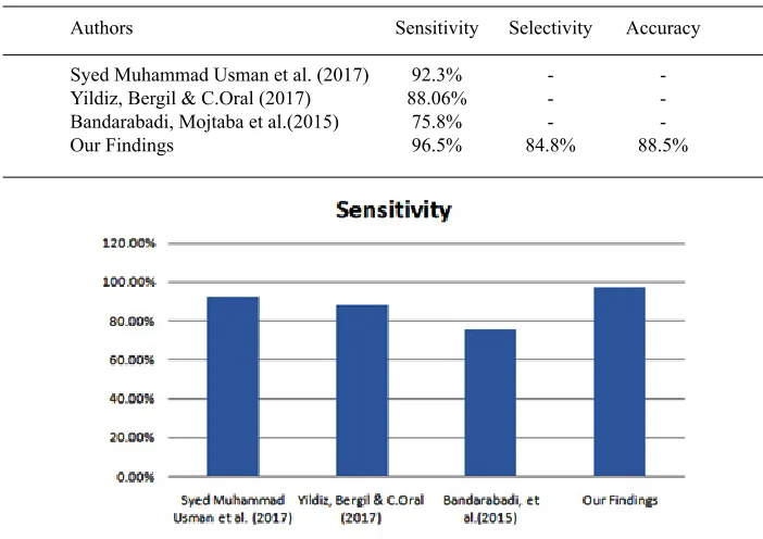
Table 3. Shows the proposed classifier output

and compare with existing techniques

Authors Sensitivity Selectivity Accuracy

Syed Muhammad Usman et al. (2017) 92.3% -

-Yildiz, Bergil & C.Oral (2017) 88.06% -

-Bandarabadi, Mojtaba et al.(2015) 75.8% -

-Our Findings 96.5% 84.8% 88.5%

Fig. 9. Shows comparison of our result with other researchers in terms of sensitivity Fig. 7. Confusion Matrix Fig. 8. ROC Curve

instances of the same class more than nearby

instances of the other class, and increases in the

reverse case.

After

k

iterations, divide each element of

the weight vector by

k

. This becomes the relevance

vector. Features are selected if their relevance is

greater than a threshold

T.

Kira and Rendell’s experiments showed

a clear contrast between relevant and irrelevant

features, allowing

T

to be determined by

inspection

_{. However, it can also be determined}

by Chebyshev’s inequality for a given confidence

make the probability of a Type I error less than

á

,

although it is stated that

T

can be much smaller

than that.

Classification using linear SVM

Support Vector Machine (SVM)

is a supervised machine learning algorithm

which can be used for both classification and

regression based problems. However, it is

mostly used in classification problems. In this

algorithm, we plot each data item as a point

in n-dimensional space (where n is number of

features you have) with the value of each feature

being the value of a particular coordinate. Then,

we perform classification by finding the

hyper-plane that differentiate the two classes very well

(look at the below snapshot) shown in Fig. 3[A].

Support Vectors are simply the

co-ordinates of individual observation. Support Vector

Machine is a frontier which best segregates the two

classes (hyper-plane/ line)

_{. In the linear case, the}

margin is defined by the distance of the hyper plane

to the nearest of the positive and negative examples.

The formula for the output of a linear SVM is

v = ѡ̄ * xˉ - b

...(1)

where w is the normal vector to the hyper

plane and x is the input vector. The separating hyper

plane is the plane v=0. The nearest points lie on the

planes v = ±1. The margin m is thus

k = 1/║ѡ║2

RESULT AnD DISCUSSIOn

This paper gives the feature extraction

results produced by applying decomposition

of signal till fifth level of IMFs by applying

HHT on EEG signals, and then RBA is used for

feature selection, followed by Linear SVM for

classification. The normal and abnormal input data

is applied after removing artifacts.

Statistical values of 29 EEG signals of

normal subjects upto 5

_{IMF has been shown in}

table 1 and values of 23 EEG signal of Epileptic

subjects has been displayed in table 2. On the basis

of these obtained values, the training and testing of

Linear SVM classifier has been proposed. 70% of

data set is used for training purpose and rest 30%

were utilised for testing results.

Once the calculation of IMFs is complete,

the following important statistical parameters are

evaluated. Table 1 & 2 are presenting the calculated

statistical values of Healthy and Unhealthy

subjects.

For feature selection Relief algorithm

calculates a feature score for each feature which

can then be applied to rank and select top scoring

features. The Hilbert–Huang transform (HHT)

is a way to decompose a signal into intrinsic

mode functions (IMF) along with a trend, and

obtain instantaneous frequency data and used for

feature extraction. For classifying the experimental

EEG signals, the Linear SVM concept has been

used. The computed statistical values are fed into

Linear SVM classifier for training and testing. The

performance of proposed methodology is evaluated

in terms of parameters of confusion matrix & ROC

Curve shown in Fig. 7 & 8.

Where TP, TN, FP and FN stands for

true positive, true negative, false positive and

false negative respectively. Sensitivity is used to

diagnose the correctly identified positive case,

specificity is defined as the determination of

negative cases accurately, selectivity is defined as

the recognition of unidentified positive results and

accuracy stands for the identification of correct

classified instances.

COnCLUSIOn

The proposed method is suitable for

separating normal and epileptic EEG data. The

com bined approach of HHT, RBAs with Linear

SVM has found to be very effective in such

classification with high sensitivity. The result of

the classification pro cess is based on using the

statistical values obtained by HHT. This technique

has been found to be suitable in the correct

classification of epileptic and healthy EEG data.

The data set is taken from Natus NeuroWorks EEG

Recording Machine from RML Institute of Medical

result shows sensitivity, selectiv ity and accuracy

are 96.5%, 84.8% and 88.5% respectively.

ACKnOWLEDGMEnT

The authors acknowledge Dr. A. K.

Thacker, Head of Department, Department of

Neurology, RMLIMS, Lucknow (U.P) for his

valuable help in developing an understanding

towards the Epilepsy. His contributions and work in

the related field helped us to think a stage ahead and

Ms. Nidhi, Technical Staff EEG Lab, RMLIMS,

Lucknow (U.P) for providing EEG Recording of

Healthy& Unhealthy Subjects.

REFEREnCES

1. R. Fisher, W. van Emde Boas, W. Blume, C. Elger, P. Genton, P. Lee, J. Engel, “Epileptic seizures and epilepsy: definitions”, Proposed by the International League Against Epilepsy (ILAE) and the International Bureau for Epilepsy (IBE), Epilepsia, 46(4): pp. 470–472 (2005). 2. R.A.S. Ruiz, R. Ranta, V. Louis-Dorr, “EEG

montage analysis in the Blind Source Separation framework”, Bio signal Processing and Control, 6(1): pp.77–84 (2010).

3. http://www.who.int/mediacentre/factsheets/ fs999/en/index.html (accessed April 2018), WHO Report

4. D. Coyle, T.M. McGinnity, G. Prasad, “Improving the separability of multiple EEG features for a BCI by neural-time-series prediction-preprocessing”, Bio-signal Processing and Control, 5(3): pp.196–204 (2010).

5. Pardey, James, Stephen Roberts, and Lionel Tarassenko. “A review of parametric modelling techniques for EEG analysis.” Medical engineering & physics 18.1 : 2-11 (1996). 6. Lange, Nicholas, and Scott L. Zeger. “Non

linear Fourier time series analysis for human brain mapping by functional magnetic resonance imaging.” Journal of the Royal Statistical Society: Series C (Applied Statistics) 46.1 : 1-29 (1997).

7. Bachmann, Maie, et al. “Non-linear analysis of the electroencephalogram for detecting effects of low-level electromagnetic fields.” Medical and Biological Engineering and Computing 43.1: 142-149 (2005).

8. Homan, Richard W., John Herman, and Phillip Purdy. “Cerebral location of international 10–20 system electrode placement.” Electroencephalography and

clinical neurophysiology 66.4 : 376-382 (1987). 9. Huang, Norden Eh. Hilbert-Huang transform and

its applications. World Scientific, 16: (2014). 10. Huang, Norden E., and Zhaohua Wu. “A review

on Hilbert Huang transform: Method and its applications to geophysical studies.” Reviews of geophysics 46.2 (2008).

11. Pachori, Ram Bilas. “Discrimination between ictal and seizure-free EEG signals using empirical mode decomposition.” Research Letters in Signal Processing, 14; (2008): 12. E. Huang, Z. Shen, and S. R. Long, “The

empirical mode decompo-sition and the Hilbert spectrum for nonlinear and non-stationary time series analysis”, in Proc. Royal Society of London Ser., 454: pp. 903–995 (1998). 13. Li, Yi, et al. “Sleep stage classification based

on EEG Hilbert-Huang transform.” Industrial Electronics and Applications, 2009. ICIEA 2009. 4th IEEE Conference on. IEEE, 2009.

14. Urbanowicz, Ryan J., et al., “Relief-based feature selection: introduction and review”, arXiv preprint arXiv:1711.08421, (2017).

15. Yu, Lei, and Huan Liu. “Feature selection for high-dimensional data: A fast correlation-based filter solution.” Proceedings of the 20th international conference on machine learning (ICML-03). (2003).

16. Sun, Yijun., “Iterative RELIEF for feature weighting: algorithms, theories, and applications”, IEEE transactions on pattern analysis and machine intelligence 29.6: (2007). 17. Sun, Yijun, Sinisa Todorovic, and Steve

Goodison. “Local-learning-based feature selection for high-dimensional data analysis”, IEEE transactions on pattern analysis and machine intelligence 32.9, pp. 1610-1626 (2010). 18. Subasi, Abdulhamit, and M. Ismail Gursoy. “EEG

signal classification using PCA, ICA, LDA and support vector machines.” Expert systems with applications 37.12: 8659-8666 (2010).

19. Amari, Shun-ichi, and Si Wu. “Improving support vector machine classifiers by modifying kernel functions.” Neural Networks 12.6 (1999): 783-789.

20. S. C. Pei and M. H. Yeh, “Discrete fractional Hilbert transform”, IEEE Trans. Circuits Syst. II, 47(11), pp. 1307–1311, (2000).

21. Barnhart, B. L., “The Hilbert-Huang transform: theory, applications, development”, (2011). 22. Flandrin, P., Rilling, G., & Goncalves, P,

“Empirical mode decomposition as a filter bank”, Signal Processing Letters, IEEE, 11(2), 112-114 (2004).

problems”, Hilbert-Huang transform and its applications, interdisciplinary mathematical sciences, 5: 1-24 (2005).

24. Fu, Kai, et al. “Classification of seizure based on the time-frequency image of EEG signals using HHT and SVM.” Biomedical Signal Processing and Control 13: 15-22 (2014).

25. Jospin, Mathieu, et al. “Detrended fluctuation

analysis of EEG as a measure of depth of anesthesia.” IEEE Transactions on Biomedical Engineering 54.5: 840-846 (2007).

26. Persson, Isac, “Feature selection of EEG-signal data for cognitive load”, (2017).