Within-sample co-methylation patterns in normal tissues

(1)

R E S E A R C H

Open Access

Within-sample co-methylation patterns in

normal tissues

Lillian Sun

1

and Shuying Sun

2*

* Correspondence:[email protected] 2

Department of Mathematics, Texas State University, San Marcos, TX, USA

Full list of author information is available at the end of the article

Abstract

Background:DNA methylation is an epigenetic event that may regulate gene

expression. Because of this regulation role, aberrant DNA methylation is often associated with many diseases. Within-sample DNA co-methylation is the similarity of methylation in nearby cytosine sites of a chromosome. It is important to study co-methylation patterns. However, it is not well studied yet, and it is unclear to us what co-methylation patterns normal DNA samples have. Are the co-methylation patterns of the same tissue across several samples different? Are the co-methylation patterns of various tissues of the same sample different? To answer these questions, we conduct analyses using two sets of data: 3-sample-1-tissue (3S1T) and 1-sample-8-tissue (1S8T).

Results:To study the co-methylation patterns of the two datasets, 3S1T and 1S8T, we

investigate the following questions: How often does one methylation state change to other methylation states and how is this change associated with chromosome distance? Based on the 3S1T data, we find there is not significant co-methylation difference among the same spleen tissues of three different samples. However, the analysis results of 1S8T data show that there were significant differences among eight tissues of one sample. For both 3S1T and 1S8T data, we find that the no/low methylation state A and high/full methylation state D tend to remain the same along a chromosome region. We also find that the low/partial methylation state B and partial/high methylation state C tend to change to higher methylation states along a chromosome. Finally, we find that lengths of most co-methylation regions are very short with only a few hundred base pairs. In fact, only a small proportion of methylated regions are longer than 1000 base pairs.

Conclusions: In this paper, we have addressed a few questions regarding

within-sample co-methylation patterns in normal tissues. Our statistical analysis results and answers may help researchers to better understand the biological process of DNA methylation. This may pave the way to develop better analysis methods for future methylation research.

Keywords: Within-sample co-methylation, Normal tissue, Statistical analysis

(2)

Introduction

Epigenetics is generally understood as the study of heritable changes that are related to gene functions and cannot be explained by changes in DNA sequences. These changes are frequently termed epigenetic events or marks. One main type of epigenetic event is DNA methylation, which is the addition of a methyl group to a 5′ cytosine base [1]. DNA methylation plays an important role in transcription and thus affects gene expres-sion [1,2]. It also plays a significant role in genomic imprinting, X-chromosome inacti-vation, and suppression of repetitive element transcription and transposition [3–7]. Therefore, it is important to study different methylation patterns in both normal sam-ples and the samsam-ples of complex diseases such as cancers.

In a human genome, DNA methylation often occurs at CpG or CG sites. A CG site is a cytosine base followed by a guanine base in DNA sequences. Because DNA methyla-tion predominantly occurs at CG sites, it is important to study DNA methylamethyla-tion at or near CpG islands, which are regions with more cytosine or CG sites. CpG islands are defined as regions of the DNA sequence > 200 bp long with an average CG content > 50% and an observed-to-expected ratio of CG sites > 0.6 [8]. These islands are import-ant regulatory elements in the genome, and contain the most variation in DNA methy-lation across different tissues. Additionally, methymethy-lation of CpG islands in promoter regions can be associated with long-term silencing of gene expression [2,9].

Researchers can study segments of methylation over a stretch of neighboring CG sites in the same chromosome region. This specific DNA methylation pattern is called co-methylation [10]. It is also called within-sample (WS) co-methylation. The prefix

“co-” in the“WS co-methylation” means local CG sites of one short chromosome

re-gion methylate or not methylate together in a single sample. That is, we study how neighboring CG sites are similarly methylated or unmethylated within a short

chromo-some region of one sample. It has also been observed that the “correlation between

methylated cytosines decays as a function of genomic distance between methylated loci”. In fact, in Arabidopsis this correlation is observed for distances up to 5000 nucle-otides [11]. For human samples, Eckhardt et al. first report that this correlation or co-methylation is over short distances (≤1000 base pairs) and it deteriorates rapidly for distances > 2000 base pairs [12]. However, this study is not conducted for the whole genome. In this paper, we will investigate in detail how long this co-methylation pattern can be in the human genome of normal samples using whole genome bisulfite sequen-cing data.

Before we introduce our study further, we emphasize that, in other research papers [13–20], co-methylation may mean “between-sample (BS) co-methylation”. The prefix “co-”in the“BS co-methylation”means that genes at different regions, especially

differ-ent chromosomes, methylate together across multiple samples. For example, “BS

co-methylation” may mean that two or more genes (e.g., genes 1 and 2) on different

chromosomes are hypermethylated together and their functions are somehow related

through a co-methylation (or co-expression) network/module [15, 19]. This

co-methylation (or“BS co-methylation”) is similar to the concept of“co-expression”of genes. The above explanations and definitions of WS co-methylation and BS co-methylation is consistent with the ones defined in Peter Francis Hickey’s thesis [21], which has a thorough review of different co-methylation definitions. It is worth noting

(3)

sample, it is important to study “WS co-methylation”across multiple samples and this is the research focus of this paper. To simplify our writing, in this paper we often use “co-methylation”for“WS co-methylation”.

It is important to study within-sample co-methylation as it explains how DNA methylation is instituted in each genomic region in a chromosome. Deep understanding of within-sample co-methylation patterns can help researchers improve DNA methyla-tion assays and statistical analyses of DNA methylamethyla-tion. Thus, we can better under-stand other genetic and epigenetic events or patterns. Although it is important to study DNA co-methylation, this specific methylation pattern has not been well studied yet. For example, it is unclear to us what co-methylation patterns normal DNA samples have. In this paper, we will conduct analyses to answer the following two questions re-garding co-methylation patterns in normal DNA. First, are the co-methylation patterns of the same tissue across several samples different? Second, are the co-methylation pat-terns of various tissues of the same sample different? In order to answer these ques-tions, we conduct analyses using two sets of data: one is 3-sample-1-tissue (3S1T), another one is 1-sample-8-tissue (1S8T). To study the co-methylation patterns of these two datasets, we specifically investigate how often one methylation state change to other methylation states and how is this change associated with chromosome distance. In the following sections, we first introduce the data we use. We then explain the two analysis methods we will use to answer the above questions. Finally, we will show our comprehensive analysis results.

Methods Data

To compare co-methylation patterns among different samples, we use a dataset of three distinct samples. The samples are referred to as STL001, STL002, and STL003 and each sample has whole genome bisulfite sequencing (WGBS) data from the spleen

tissue. These datasets are obtained from the Roadmap Epigenomics Project [22]. We

refer to this dataset as 3-sample-1-tissue, or 3S1T. To compare co-methylation patterns among different tissues of the same sample, we use a dataset of eight distinct tissues of the sample STL001. The eight tissues are respectively referred to as bladder, gastric, lung, psoas, sigmoid colon, small bowel, spleen, and thymus. This dataset is obtained from Roadmap Epigenomics Project [22]. We refer to this dataset as 1-sample-8-tissue, or 1S8T. For both 3S1T and 1S8T data, the raw WGBS reads are preprocessed and aligned using BRAT-bw [23], a publicly available software package, and the human gen-ome hg19 is used as the reference gengen-ome. Because our focus is within-sample co-methylation for nearby sites or regions, not between-sample co-methylation in a whole genome, using one chromosome is sufficient to address the questions of interest. Therefore, we only focus on chromosome 1, as it is the longest chromosome. In fact, we use methylation ratios from all CG sites in chromosome 1 of each dataset.

(4)

is the proportion of sequenced reads of a CG site that are methylated. 0 indicates no methylation and 1 indicates full methylation. We then add a fifth metric—the methyla-tion state of each CG site—to all datasets.“Methylation state”refers to each of our divi-sions of the MC ratio [0,1] into four intervals of methylation. These methylation states are A, B, C, and D. “A”corresponds to no/low MC ratios of [0, 0.25).“B” corresponds to low/partial MC ratios of [0.25, 0.5). “C” corresponds to partial/high MC ratios of [0.5, 0.75).“D” corresponds to high/full MC ratios of [0.75, 1]. CG sites with a sequen-cing coverage of less than 3 (i.e., <3X) are labeled “NA”. Note, as for the sequencing coverage, for all datasets (samples/tissues), around 95% of CG sites have at least 1X

coverage. Only two samples/tissues have 89 and 91% of CG sites with ≥3X coverage.

All other samples/tissues have about 95% of CG sites with≥3X coverage. Lastly, we cal-culate the distance between consecutive CG sites and add these values in the final

col-umn of our data (Table 1). “Consecutive CG sites” mean two CG sites on the same

chromosome and at the same DNA strand, that is, there is no other CG site between them. The first and second CG sites are determined based on the reference genome co-ordinates on the positive or forward strand. In this paper, we only use the positive or forward strand of the DNA.

Two analyses

We prepare the original data as described above, labeling the methylation state of each CG site and calculating distance between consecutive CG sites, so that we may use them in our two analyses. First, we investigate how frequently methylation states change from one CG site to another along a chromosome. Second, we investigate if this change is related to chromosome distance.

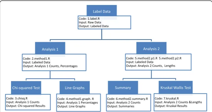
We would like to investigate patterns beyond the scope of single sample or sue. Do the co-methylation patterns vary across different samples or different tis-sues? We apply our analyses to the different samples and tissues in two datasets, 3S1T and 1S8T. We compare co-methylation patterns across different samples in 3S1T and compare co-methylation across different tissues in 1S8T to answer these questions. The workflow of our analyses is shown in Fig. 1. Next, we explain in de-tail each analysis method.

Analysis 1

In our first analysis, we analyze how methylation patterns change from one CG site to another. Since each CG site has a methylation state assigned to it according to its

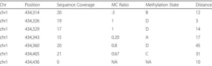
Table 1Sample section of data

Chr Position Sequence Coverage MC Ratio Methylation State Distance

chr1 434,314 20 .3 B 12

chr1 434,326 19 1 D 3

chr1 434,329 17 1 D 14

chr1 434,343 15 0.20 A 17

chr1 434,360 20 0.8 D 45

chr1 434,405 21 0.67 C 31

(5)

methylation level, we pair together consecutive CG sites along the genome to form a “methylation state pair”—the two states corresponding to a pair of CG sites. This allows us to observe how methylation can change along a chromosome region. The first state indicates the initial methylation level, while the second state indicates the terminal methylation level. Does methylation stay the same (e.g., AA, BB, CC, DD), relatively similar (e.g., AB, CD), or change drastically (e.g., AD, DA)? Do certain methylation states tend to change to other methylation states?

For each sample, we also calculate the frequency of the distinct state pairs (e.g., AA, AB, AC, AD). This allows us to compare the co-methylation patterns across different samples or tissues (see Chi-squared test below). We learned from our previous research that co-methylation patterns are related to the physical distance between two CG sites in a state pair. Thus, we calculate the frequency of each type of methylation state-pair at increasing intervals of a short distance of 50 bases, i.e., [0, 50), [50, 100), [100, 150), …, [400, 450), [450, 500), to [500, Inf ). We then graph the frequencies of different sam-ples or tissues with the same methylation state pair on the same graph to visually ob-serve differences. We also utilize the chi-squared test to determine whether samples or tissues are significantly different. We first test all samples or tissues at once. If there is a significant difference, we further analyze the data by pairwise comparison to deter-mine which combination of samples may be the cause of the difference. If the p-values are extremely small, we may use or combine approaches below to produce better ana-lysis results.

a) We calculate the contribution of each methylation state pair and each sample to a Chi-squared statistic. This allows us to determine which sample and which methy-lation state pair is the most significantly different from the others. We display this information in bar graphs for visualization.

b) We divide our methylation state-pair count data (i.e., Chi-squared input) by factors of n (n= 10, 100, 1000) to account for large-count issues.

(6)

Analysis 2

In our second analysis, we investigate how long methylation levels stay the same in a chromosome by analyzing the length of similarly methylated regions. We begin by grouping together consecutive CG sites that have the same methylation state (e.g., AAAA, BBBB, CCCC, or DDDD). These groups are called similarly methylated regions (SMRs). We then calculate the number of CG sites in each group (count) and the num-ber of base pairs the group stretches across (region-length or length). These two values are used as metrics that we use to compare different samples or tissues.

Once we calculate counts and lengths, we summarize the counts and lengths of the four different SMRs: A, B, C, and D. We summarize SMRs with a count of at least two CG sites. We then determine whether SMRs from different samples or tissues with the same methylation level (i.e., AAAA in Bladder and AAAAA in Thymus) have signifi-cantly different distributions of lengths or of counts. We begin to analyze SMR count/ length summaries across different samples or tissues. These summaries provide a pre-liminary assessment of whether SMR lengths and counts from different tissues or sam-ples may differ. We then use the Kruskal Wallis test to confirm any significant differences, first comparing all samples or tissues and then conducting pairwise com-parisons, if necessary.

Results

3S1T data analysis results

First, we show the results of analyzing if different samples of the same tissue have dif-ferent co-methylation patterns.

Analysis 1 result of 3S1T data

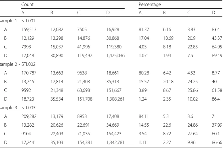
We have labeled and paired consecutive CG sites in the data to form methylation state pairs. Table2 displays the number of times each methylation state pair occurs and the relative frequency of methylation state pair. With this summary, we can answer the questions about how methylation changes from one methylation state to another.

For the STL001 spleen data in Table 2, methylation state pair DD occurs the most

(89.49%), followed closely by the methylation state pair AA (81.37%). This means that no/low (A) or high/full (D) methylation states in the STL001 spleen sample tends to stay within the same methylation state. For example, when looking at just row A, across columns A, B, C, and D, the no/low methylation state A tends to remain the same methylation state, no/low (A). On the other hand, low/partial methylation state B and partial/high methylation state C tends to change to higher methylation states: C and D. For high/full methylation state D, the methylation tends to remain high/full (D). There is not a large percentage of methylation state change from D to A (only about 1%). The STL002 and STL003 spleen samples follow similar patterns with some variation in the actual values.

Comparing co-methylation patterns among 3 samples of the spleen tissue (i.e., 3S1T data)

(7)

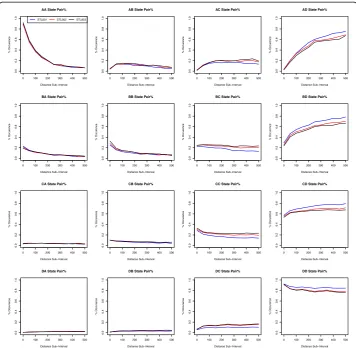
significant, see Fig.2. Plots in Fig.2do not display an obvious difference in change pat-terns among the three spleen datasets. The three lines depicting each sample do not vary from each other greatly, except that there is a bit of variation between samples in the higher methylation states, e.g., AD, BD, CD, and DD state pairs.

Next, we use chi-squared tests to study whether there are statistically significant dif-ferences for the co-methylation patterns of three samples. The null (H0) and alternative (Ha) hypotheses of the chi-squared tests are listed below. H0: There is no difference for the co-methylation patterns among the spleen tissue of three samples. That is, the methylation state change patterns from each methylation state (e.g., A) to all states (A, B, C, D) are the same among the spleen tissues of three samples. Ha: There are differ-ences for the co-methylation patterns among the spleen tissue of three samples. We

use our original count data in Table 2 as the input for each sample to conduct the

chi-squared test. We first test all three samples for differences. If the results for all three are significant, we will determine which subset of samples are different: we fur-ther test pairs of samples.

The chi-squared test results for all three spleen samples of 3S1T dataset are shown in Table3. Thep-values are very small, almost zero. As indicated above, we then conduct pair-wise comparisons between each two of the three samples and we still obtain

ex-tremely small p-values (data not shown), which shows that three spleen samples are

statistically different. However, we suspect that there may be some outlying co-methylation patterns that causes our p-value to be extremely small. Therefore, we compare the chi-squared contributions of each of the co-methylation patterns, see Table 4and Fig.3. Table 4 shows that in each of the three samples, some methylation

Table 2Methylation state change of the 3S1T data

Count Percentage

A B C D A B C D

sample 1 - STL001

A 159,513 12,082 7505 16,928 81.37 6.16 3.83 8.64

B 12,129 13,298 14,876 30,868 17.04 18.69 20.9 43.37

C 7398 15,037 41,996 119,380 4.03 8.18 22.85 64.95

D 17,048 30,890 119,492 1,425,036 1.07 1.94 7.5 89.49

sample 2 - STL002

A 170,787 13,663 9638 18,661 80.28 6.42 4.53 8.77

B 13,745 17,814 21,403 35,313 15.57 20.18 24.25 40

C 9592 21,348 63,698 151,667 3.89 8.67 25.86 61.58

D 18,723 35,534 151,708 1,308,261 1.24 2.35 10.02 86.4

sample 3 - STL003

A 209,282 13,179 8953 17,408 84.11 5.3 3.6 7

B 13,282 20,626 22,691 34,669 14.55 22.6 24.86 37.99

C 9104 22,403 71,035 154,423 3.54 8.72 27.64 60.1

D 17,244 35,103 154,381 1,342,781 1.11 2.27 9.96 86.66

(8)

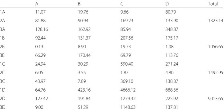
state pairs contribute more than others. For example, the DC methylation-state-pair contributions of spleen samples 1, 2, and 3 are significantly higher than other methyla-tion state pairs. They are 4666.12, 1279.32, 1148.63, as shown in the fourth column of the bottom panel of Table4.

In Fig. 3, the turquoise, dark green, and orange bars on the “by.sample” bar graphs display the primary contributions–how each methylation state pair contributes to the

Fig. 2Comparing co-methylation patterns among three spleen samples (for 3S1T data). These graphs are created by plotting the percent occurrence for each distance sub-interval incremented by 50: [0, 50), [50, 100), [100, 150), and so on to [500, Inf). The x-axis indicates distance between CG sites. For example, a distance sub-interval of [50, 100) means that all paired CG sites are within 50 to 100 base pairs of each other. The y-axis indicates the percent occurrence of the methylation state pair as designated by the graph title. The solid red line, the dashed blue line, and the dotted black line indicate the trend of the STL001, STL002, and STL003 spleen sample respectively

Table 3Chi-squared test results of 3S1T data

A B C D

p-value 1.06E-282 4.98E-225 1.80E-319 0

Chi-square 1323.14 1056.65 1492.95 9013.65

Degree of freedom 6 6 6 6

(9)

chi-squared statistic. The“by.sample”graphs can also indicate secondary contributions. That is, how much each individual sample contributes to the primary methylation state pair contributions. The blue, red, green and purple “by.methy.state”bar graphs display

the primary contributions (per bar) – how each sample contributes to the entire

chi-squared test statistic. The graphs also indicate secondary contributions within each bar. That is, how much each methylation state pair contributes to the primary sample contribution. The length of the bar or bar-segment corresponds to the amount of con-tribution to the overall chi-squared statistic by a specific sample or methylation state. Our analysis results show that for co-methylation patterns with methylation state pairs

Table 4Contributions of each methylation state pair to chi-squared values (for 3S1T data)

A B C D Total

1A 11.07 19.76 9.66 80.79

2A 81.88 90.94 169.23 133.90 1323.14

3A 128.16 162.92 85.94 348.87

1B 92.44 131.37 207.56 175.17

2B 0.13 8.90 19.73 1.08 1056.65

3B 66.29 170.44 69.79 113.76

1C 24.94 30.29 590.40 271.24

2C 6.05 3.55 1.87 4.80 1492.95

3C 43.97 7.89 369.10 138.87

1D 64.76 423.16 4666.12 688.36

2D 127.42 191.84 1279.32 225.92 9013.65

3D 9.00 51.29 1148.63 137.81

Each cell corresponds to a methylation state pair. The row indicates the sample and initial methylation state. 1 corresponds to STL001 spleen, 2 to STL002 spleen, and 3 to STL003 spleen. The column indicates the terminal methylation state. Numerical values indicate the chi-squared contribution of a methylation state pair to the chi-squared test comparing all state pairs that begin with the same state (e.g., AA, AB, AC, AD). For example, the first number (11.07) is sample 1’s (STL001) AA pair’s contribution to the chi-squared test statistic (1323.14 in Table3’s column A and Table4’s last column)

(10)

that start with B, C, and D, sample 1 or STL001 contributes the most (see the green or

bright green bars in “B/C/D.contr.by.methy.state”). Thus, in regards to the

co-methylation patterns of methylation state changes starting with B, C, and D, STL001 has the patterns that are the most different. However, for the co-methylation pattern of methylation state changes starting with A, sample 3 or STL003 is the most different one, see the last/fourth orange bar in the “A.contr.by.sample”of Fig.3top left panel.

Both the 3-sample chi-squared test result (i.e., small p-values in Table 3) and the

above “contribution” Fig. 3 and Table 4 show that the three spleen samples have

significantly different co-methylation patterns. These results seem to be

contradict-ory with our intuitive findings shown in Fig. 2, that is, these 3 samples are not

very different. This discrepancy, especially the very significant p-value may be caused by a large-count or large sample size effect, since chromosome 1 is very long, including 2,284,470 CG sites. Under the assumption that a subset of our chromosome is representative of the entire chromosome, we divide the analysis 1 count data (the left panel of Table 2) by 10s (by 1, 10, 100, and 1000). This helps to lessen the potential effect of a large sample size, as this “dividing” method cre-ates a simulated 100, 10, 1%, and .1% of our data. For example, the STL001 AA

count in Table 2 is originally 15,913, but after dividing by 10, it becomes 1591;

After dividing by 100, it becomes 159.

Once we divide our method 1 data (the methylation state pair counts) by these factors of 10, we run the chi-squared test on the “modified” count data. We

deter-mine whether the p-values remain significant as the data pool gets smaller. If we

see that the p-value becomes less significant as the sample size becomes smaller, we may conclude that the original p-values are not accurate due to a large sample size. The results will also tell us whether the methylation-change patterns between our three samples are significantly different. Our data for the chi-squared tests on

all three spleen samples are shown in Table 5. We find that the test results

be-come less significant as the sample size decreases. This shows that we do initially

get a very small p-value because of the large sample size effect. We can determine

that there is not a confirmation of a significant difference in the co-methylation patterns of three spleen samples. The patterns we observed in our Analysis 1 result may be applicable to other spleen samples, if confirmed by future studies with more normal spleen samples.

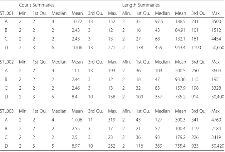
Analysis 2 results of 3S1T data

To analyze and compare how long SMRs are, we gather 6 summary values: the mini-mum, 1st Quartile, median, mean, 3rd Quartile, and maximini-mum, for the number of CG sites (count) and distance in base pairs (length) for each SMR in each sample. Note, to avoid the impact of an extreme outlier, we remove the largest count/length and summarize our counts and lengths in Table 6. This table displays the distribution of count and length so that we can visualize and compare the distribution among our

three spleen samples. Table 6 shows that the distributions of SMR length or

(11)

pairs for state D. The median count among SMRs is about 2 to 6 CG sites. Only a small proportion (< 25%) of the SMRs are longer than 1000 base pairs.

The summary in Table 6 will help us to determine whether there are any significant differences among the three samples. Table6shows that the right-skew patterns of the A, B, and C methylation-state count vary among three spleen samples. We also notice that the SMRs of methylation state D are an exception to Cokus et al’s paper [11], where they observe a correlation between methylated cytosines for distances up to 5000 bases in Arabidopsis. The D regions can reach up to 50,000 bases in a human

Table 5Chi-squared test results after addressing the large-count issue (for 3S1T data)

Division Value A B C D

1 p-value 1.06E-282 4.98E-225 1.80e-319 0

Chi-square 1323.14 1056.65 1492.95 9013.66

10 p-value 4.17E-26 1.64E-20 1.07E-29 1.92E-191

Chi-square 132.32 105.67 149.33 901.34

100 p-value 0.041 0.11 0.021 2.94E-17

Chi-square 13.13 10.42 14.93 90.06

1000 p-value 0.95 0.98 0.96 0.16

Chi-square 1.64 1.19 1.48 9.3

Degree freedom 6 6 6 6

The rows indicate the factor that the data are divided by. The second column indicates the type of value from the chi-squared test. The remaining columns indicate which co-methylation pattern the chi-chi-squared test is used to compare

Table 6SMR summaries of 3S1T data

Count Summaries Length Summaries

STL001 Min. 1st Qu. Median Mean 3rd Qu. Max. Min. 1st Qu. Median Mean 3rd Qu. Max.

A 2 2 4 10.72 13 152 2 35 97.5 188.5 231 3500

B 2 2 2 2.43 3 12 2 16 43 84.91 101 1512

C 2 2 2 2.43 3 13 2 27 68 132.1 161 4454

D 2 3 6 10.06 13 221 2 138 459 943.4 1190 50,660

A 2 2 4 11.1 13 193 2 36 103 200.5 250 3604

B 2 2 2 2.44 3 12 2 18 47 93.36 115 1951

C 2 2 2 2.46 3 13 2 32 83 157.9 198 3328

D 2 3 5 8.4 10 158 2 109 357 735.2 914 50,400

A 2 2 4 17.06 11 319 2 43 127 300.3 341 4760

B 2 2 2 2.55 3 17 2 21 52 100.4 119 2184

C 2 2 2 2.5 3 23 2 36 93 179.2 226 3419

D 2 3 5 8.97 10 252 2 116 369 755.4 925 50,420

(12)

sample. Next, we investigate more on this question: Are these distribution differences significant? We answer this question using Kruskal Wallis tests.

Comparing the distribution of the count and length of SMRs across three spleen samples

We use the Kruskal Wallis test to analyze whether there is a significant difference between the distribution of count and length of the SMRs for each methylation state of each sample. The null (H0) and alternative (Ha) hypotheses of the Kruskal

Wallis test are listed below. H0: The CG count (or length) distribution of SMRs

are the same among three samples. That is, there is no difference among the CG

count distribution of the three samples. Ha: There are differences for the SMR CG

count distribution among the spleen tissue of three samples. We use our original

count data, which are summarized in Table 6, as input for each sample to conduct

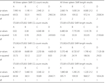
the Kruskal Wallis test. The test results are shown in Table 7. As displayed in this

table, most of the p-values are very small, except for two p-values in the

STL001vSTL002 comparison. This finding means that the three spleen samples are significantly different regarding the distribution of SMR length and the distribution of SMR CG-site count.

1S8T data analysis results

After addressing whether different samples of the same tissue have significantly differ-ent co-methylation patterns using the 3S1T data, we next show the results of

Table 7Kruskal Wallis results of 3S1T data

All three spleen SMR CG count results All three spleen SMR length results

A B C D A B C D

p-values 7.99E-16 1.19E-11 2.94E-21 0 2.06E-74 1.83E-24 8.00E-212 0

x-squared 69.53 50.31 94.55 2965.34 339.34 109.32 972.14 2508.34

df 2 2 2 2 2 2 2 2

STL001vSTL002 SMR CG count results STL001vSTL002 SMR length results

A B C D A B C D

p-values 0.02 0.38 6.04E-08 0 6.48E-04 7.77E-09 1.51E-78 0 x-squared 5.35 0.78 29.35 2459.83 11.63 33.33 352.05 2130.60

df 1 1 1 1 1 1 1 1

A B C D A B C D

p-values 6.33E-09 8.68E-09 2.25E-06 4.60E-03 5.57E-48 8.72E-07 1.79E-42 7.12E-08 x-squared 33.73 33.12 22.37 8.03 211.80 24.19 186.56 29.03

df 1 1 1 1 1 1 1 1

A B C D A B C D

p-values 8.29E-17 5.46E-10 3.34E-22 0 1.88E-68 1.20E-25 1.22E-212 0 x-squared 69.34 38.51 93.89 2040.71 305.71 109.59 968.57 1654.28

df 1 1 1 1 1 1 1 1

(13)

investigating if different tissues of the same sample have significantly different co-methylation patterns using the 1S8T data.

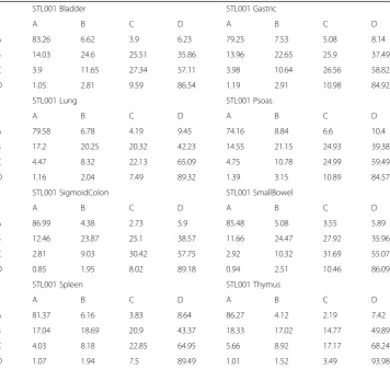
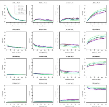
We can analyze this dataset in two ways. First, we look at the overall theme for all eight tissues; we want to figure out which methylation state pair occurs most frequently. As shown in Table8, for the bladder data, the AA methylation state pair has a percentage of 83.26% and the DD methylation state pair has a percentage of 86.54%. We notice that the different tissues display similar patterns; the AA and DD methylation state pairs have the highest percentage. We find that methylation tends to remain within the same methylation level if it is high or low. On the other hand, medium levels of methy-lation trend towards higher methymethy-lation states. This pattern continues throughout all eight tissues. However, there is some variation or difference among these eight tissues. We will investigate how closely these eight tissues follow the patterns we observed, so we graph percentage data for each tissue at certain distance intervals, see Fig. 4. This figure shows that there are some differences among those 8 tissues, especially for AD, BD, CD, and DD state pairs.

Table 8Methylation state change of 1S8T data

STL001 Bladder STL001 Gastric

A B C D A B C D

A 83.26 6.62 3.9 6.23 79.25 7.53 5.08 8.14

B 14.03 24.6 25.51 35.86 13.96 22.65 25.9 37.49

C 3.9 11.65 27.34 57.11 3.98 10.64 26.56 58.82

D 1.05 2.81 9.59 86.54 1.19 2.91 10.98 84.92

STL001 Lung STL001 Psoas

A B C D A B C D

A 79.58 6.78 4.19 9.45 74.16 8.84 6.6 10.4

B 17.2 20.25 20.32 42.23 14.55 21.15 24.93 39.38

C 4.47 8.32 22.13 65.09 4.75 10.78 24.99 59.49

D 1.16 2.04 7.49 89.32 1.39 3.15 10.89 84.57

STL001 SigmoidColon STL001 SmallBowel

A B C D A B C D

A 86.99 4.38 2.73 5.9 85.48 5.08 3.55 5.89

B 12.46 23.87 25.1 38.57 11.66 24.47 27.92 35.96

C 2.81 9.03 30.42 57.75 2.92 10.32 31.69 55.07

D 0.85 1.95 8.02 89.18 0.94 2.51 10.46 86.09

STL001 Spleen STL001 Thymus

A B C D A B C D

A 81.37 6.16 3.83 8.64 86.27 4.12 2.19 7.42

B 17.04 18.69 20.9 43.37 18.33 17.02 14.77 49.89

C 4.03 8.18 22.85 64.95 5.66 8.92 17.17 68.24

D 1.07 1.94 7.5 89.49 1.01 1.52 3.49 93.98

(14)

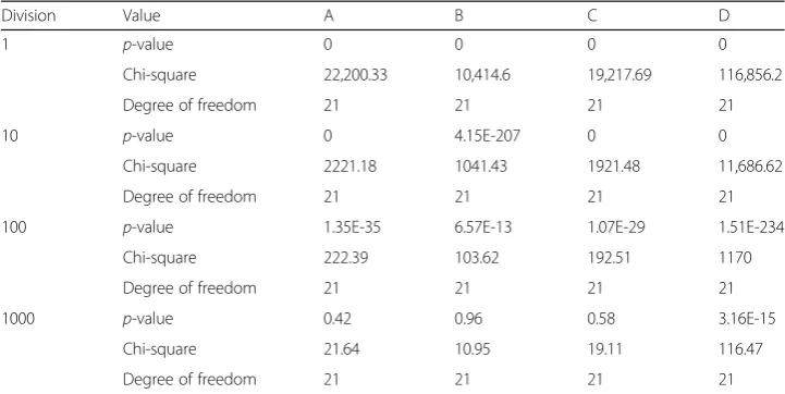
Next, we conduct chi-squared tests to compare the 8 tissues, see the top panel of “divide by 1” in Table 9. When comparing all eight tissues together, we find that there are statistically significant differences in the co-methylation patterns among 8 tissues. To avoid the large-count issue, we divide the input data by factors of 10: 1, 10, 100, and 1000 as we did for the 3S1T data. The division of the data by 100 seems to help the results to be more accurate. As for the division by 1000, the count (or expected count for the chi-square test) is less than 5, so we will not use this result. Instead, we use the results with the division by 100, which still shows

there are small p-values, that is, the 8 tissues have significantly different

co-methylation patterns.

We also try to break the chi-squared test results down into the contributions that each methylation state and/or tissue contributes to the chi-squared value. We would like to know if any one tissue/methylation state has a bigger effect on the chi-squared test, and if so, whether we should remove that tissue/methylation state as an outlier. We display our Analysis 1 chi-squared contribution using bar graphs, see Fig.5. In this

(15)

figure, we can see that the 8th tissue, thymus, contributes most to the difference. We can also see that the 4th tissue, Psoas, contributes occasionally. We remove the 8th tis-sue, thymus, from our dataset, and re-run the chi-squared test on our data to see if the results are more accurate. Our results are displayed in Table 10. We can see that the

p-values for this test remain zero, even though we remove a tissue. So, we try to divide the chi-squared input of the seven tissues by factors of 10, similar to what we have done above, and observe the chi-squared results. The result of dividing by 100 still have significant difference among 7 tissues; however, the results of dividing by 1000 only show a significant difference for D states, but not for A, B, or C states.

Table 9Chi-squared test results divided by factors of 10 (for 8 tissues of 1S8T data)

1 p-value 0 0 0 0

Chi-square 22,200.33 10,414.6 19,217.69 116,856.2

10 p-value 0 4.15E-207 0 0

Chi-square 2221.18 1041.43 1921.48 11,686.62

100 p-value 1.35E-35 6.57E-13 1.07E-29 1.51E-234

Chi-square 222.39 103.62 192.51 1170

1000 p-value 0.42 0.96 0.58 3.16E-15

Chi-square 21.64 10.95 19.11 116.47

The rows indicate the factor that the data are divided by. The second column indicates the type of value from the chi-squared test. The remaining columns indicate which co-methylation pattern the chi-chi-squared test is used to compare. Note, the meaning or interpretation of this table is similar to Table5, which is for the 3S1T data

(16)

We would like to analyze SMRs. We first group CG sites that are similarly methylated and determine the number or count of CG sites in each SMR and the length (in base pairs) of each SMR. We then create summaries of the CG site number count and

length of SMRs, see Table 11. Similar to Table 6 (summary for 3S1T data), Table 11

shows that the distributions of SMR length or CG-number count skew to the right. Most SMRs are very short. The median SMR length is around 100 to 130 base pairs for methylation state A and 300 to 500 base pairs for state D of all tissues except thymus. The median count among SMRs is about 2 to 6 CG sites. Next we determine whether SMRs of the same methylation level have different counts/lengths.

We run the Kruskal Wallis test on all eight tissues to determine if the distribution of counts and distances of each type of SMR are significantly different. Our initial results are displayed below in Table 12. As we can see, thep-values for the count in columns C and D, and the p-values for distance in columns A, C, and D are all nearly zero. The remaining p-values are also extremely small. This shows that those 8 tissues are signifi-cantly different.

In summary, in the Result section, we have shown the results of analyzing two data-sets, 3S1T and 1S8T, to address a few questions mentioned in the Introduction section.

Discussion

Our research work is a specific study with a focus on the analysis of within-sample co-methylation patterns in normal DNA samples. The understanding of this specific type of methylation patterns may provide helpful information and insights on other methylation studies. These studies may include the analysis of methylation patterns for specific genes or regions (e.g., long non-coding RNAs [16]), identifying differential methylation [24–27],classifying large methylation data [28–30],integrating methylation with other data (e.g., gene expression data) [31–33], and analyzing pan-cancer DNA methylation [20,34–37].

Table 10Chi-squared test results of 7 tissues divided by factors of 10 (for 1S8T data)

1 p-value 0 0 0 0

Chi-square 17,285.29 5441.81 14,025.19 41,241.11

10 p-value 0 5.53E-104 5.10E-287 0

Chi-square 1729.24 544.06 1402.08 4124.86

100 p-value 2.50E-27 1.73E-05 4.86E-21 1.62E-76

Chi-square 172.84 54.16 140.62 413.19

1000 p-value 0.55 1 0.72 1.40E-03

Chi-square 16.58 5.8 14.19 41.28

(17)

Table 11SMR summaries of 1S8T data

Bladder Count Summaries Bladder Length Summaries

Min. 1st Qu. Median Mean 3rd Qu. Max. Min. 1st Qu. Median Mean 3rd Qu. Max.

A 2 2 4 15.59 11 344 A 2 40 121 283.7 331 8693

B 2 2 2 2.54 3 16 B 2 24 62 117.9 148 2061

C 2 2 2 2.49 3 13 C 2 32 84 157 201 2882

D 2 3 5 9.03 11 213 D 2 118 390 789.4 1003 100,200

Gastric Count Summaries Gastric Length Summaries

A 2 2 4 10.66 12 170 A 2 34 95 193.7 239 5156

B 2 2 2 2.48 3 15 B 2 22 57 109.5 136 2534

C 2 2 2 2.46 3 15 C 2 31 82 585 202 21,050,000

D 2 3 5 7.74 10 146 D 2 102 335 665.6 853 50,630

Lung Count Summaries Lung Length Summaries

A 2 2 4 9.33 11 137 A 2 34 92 176.5 220 5765

B 2 2 2 2.44 3 11 B 2 18 45 87.52 106 1549

C 2 2 2 2.4 3 14 C 2 26 66 875 161 21,050,000

D 2 3 6 9.68 12 208 D 2 135 447 908.6 1162 100,200

Psoas Count Summaries Psoas Length Summaries

A 2 2 4 8.23 9 132 A 2 30 83 157.7 193 4512

B 2 2 2 2.42 3 12 B 2 21 54 106.1 128.8 2690

C 2 2 2 2.41 3 12 C 2 29 77 152.1 189 3643

D 2 3 5 7.42 9 169 D 2 95 315 652.1 824 100,300

SigmoidColon Count Summaries SigmoidColon Length Summaries

A 2 2 4 22.19 20 374 A 2 42 136 351.7 428 5156

B 2 2 2 2.64 3 25 B 2 20 52 96.21 121 1835

C 2 2 2 2.69 3 48 C 2 34 86 678 201 21,050,000

D 2 3 6 10.65 13 294 D 2 150 488.5 963.3 1227 100,200

SmallBowel Count Summaries SmallBowel Length Summaries

A 2 2 4 20.62 17 390 A 2 42 132 340.6 397 8889

B 2 2 2 2.62 3 38 B 2 23 59 108.5 135 1714

C 2 2 2 2.66 3 34 C 2 37 95 560 226 21,050,000

D 2 3 5 8.68 10 233 D 2 117 375 735.5 940 50,460

Spleen Count Summaries Spleen Length Summaries

A 2 2 4 10.73 13 164 A 2 35 98 188.8 231 4941

B 2 2 2 2.43 3 14 B 2 16 43 85.06 101.8 1534

C 2 2 2 2.43 3 14 C 2 27 68 851 161 21,050,000

D 2 3 6 10.06 13 265 D 2 138 459 944 1190 100,200

Thymus Count Summaries Thymus Length Summaries

(18)

To the best of our knowledge, there is not much research work done on the WS co-methylation patterns of normal DNA samples, although there are a larger number of papers on BS co-methylation. Thus, in this paper, we conduct some preliminary ana-lyses on WS co-methylation for normal samples. However, our research work has cer-tain limitations. First, this study is only conducted on normal samples, but this type of within-sample analysis can be performed on other datasets, for example, cancer methy-lation data with multiple samples. In fact, we have submitted a paper on comparing the within-sample co-methylation between normal and cancer samples. In that paper, we find that the breast cancer sample’s co-methylation pattern is very different from the patterns reported in this manuscript. But the breast normal sample has a similar tern as we found in the 1S8T data of the current study. Therefore, co-methylation pat-terns of other normal samples or other datasets could be very similar to what we showed as we used a relatively large number of different normal tissues in this paper. The second limitation is that our study is only based on basic statistical analysis. More complex probability models (e.g., Hidden Markov Models) and methods (e.g., Bayesian methods or machine learning) may be used to further investigate within-sample co-methylation. Developing a new method based these ideas and methods is beyond the scope of this paper. However, we do plan to implement these models and ideas in other projects in the near future. The third limitation is that we did not investigate the relationship between WS co-methylation and the genomic context and/or the topology of CG sites [38]. It would be biologically meaningful to investigate in detail how WS co-methylation patterns are related to the genomic compartments, e.g., gene body, gene promoter, and CpG islands. To make it easier for other readers to interpret the co-methylation CG sites or patterns, we provide an annotation code (annotation.R) in the Additional File 1that can report the location of identified CG sites, that is, which gene body or promoter it belongs to. Note, the Additional File 1 includes all R scripts we wrote for the analysis of this paper. In addition, it is also useful to study how these patterns are related to the density of CG sites (or CG clusters) in an entire genome and study how CG sites collaborate to maintain co-methylation patterns [38,39]. These are

Table 11SMR summaries of 1S8T data(Continued)

B 2 2 2 2.44 3 23 B 2 14 36 72.25 86 1443

C 2 2 2 2.36 2 20 C 2 20 51 102.1 118 2152

D 2 4 9 17.04 21 408 D 2 229 818 1696 2120 100,200

The first column designates the type of SMR. The remaining columns are the summary. For example, for the bladder tissue, the“A”row (i.e., the 3rd row) is the summary of the“AA…A”type SMR’s count and length, and the“B”row (4th row) is the summary of the“BB…B”type SMR’s count and length of this tissue

Table 12Kruskal Wallis test results of 1S8T data

SMR CG Site Count SMR Length

A B C D A B C D

p-values 6.73E-97 3.13E-91 0 0 0 1.79E-260 0 0

x-squared 467.78 441.39 2645.20 32,987.79 2168.20 1225.88 3020.88 29,507.40

df 7 7 7 7 7 7 7 7

(19)

all great aspects to investigate further in future research studies and we do plan to con-duct research on these topics.

In order to confirm the validity of our findings, we have also conducted our analysis on the same tissues and samples from chromosome 2. We find similar patterns and can make the same conclusion. In order to avoid redundancy, we do not show the re-sults of chromosome 2 data analysis and only show the rere-sults of analyzing chromo-some 1 in this paper.

Conclusion

In this paper, we have conducted analyses to study the within-sample co-methylation patterns in normal DNA samples. We have investigated if the co-methylation patterns of the same tissue across several samples are different and if the co-methylation pat-terns of various tissues of the same sample are different. We have used two analyses methods to analyze two datasets, 3S1T and 1S8T. Based on the 3S1T data, we find there is not significant co-methylation difference among the same spleen tissues of three different samples. However, the analysis results of 1S8T data show that there were significant differences among eight tissues of one sample. For both 3S1T and 1S8T data, we find that the no/low methylation state A and high/full methylation state D tend to remain the same along a chromosome region. We also find that the low/par-tial methylation state B and parlow/par-tial/high methylation state C tend to change to higher methylation states along a chromosome. Furthermore, we find that the distribution of SMR length is skewed to the right and most SMRs are very short (with only a few hun-dred base pairs) and only a small proportion of SMRs are longer than 1000 base pairs. In this paper, we have addressed a few questions regarding within-sample co-methylation. Our answers and analysis results may help researchers to have a deep understanding of co-methylation patterns and thus to improve DNA methylation assays and statistical analyses for other methylation studies.

Abbreviations

CG:Cytosine-guanine; SMR: Similarly methylated region; WGBS: Whole genome bisulfite sequencing

Acknowledgements

This project was completed with the use of Texas State University facilities and resources. This work was also supported by Dr. Sun’s Texas State University Research Enhancement Program (REP) grant. We appreciate that Brittany Sue Enfield helped us find the data used in this paper when she was working on her honors thesis with Dr. Sun at Texas State University.

Funding

This project is supported by the Texas State University Research Enhancement Program.

Availability of data and materials

Datasets used in this paper are publicly available with detailed information shown below. In particular, we provide the web links for the raw sequencing data, on which all SRA (Short Read Archive) files are available, see below. These links are useful for readers like us, who would like to process raw sequencing reads to obtain methylation signals by themselves. Besides the web links of SRA files, we also provide GEO (Gene Expression Omnibus) web links, on which the processed methylation signal datasets (e.g., hg19 version wig format files) are available now or may be available later. Note, for some of the GEO web links, the processed methylation signals are not available yet. When we search the processed methylation signal data, we find that the original investigators who generated these datasets mentioned that“various levels of processed data files will be made available as this project proceeds”. Therefore, readers who are interested in the processed methylation data may check the GEO web sites later. In addition, readers can also visithttp:// www.encodeproject.org, click“Experiments”, and then select related search items (e.g., WGBS and spleen) to find more information about a specific dataset.

# 3S1T data (3 spleen tissue of STL001, STL002, and STL003)

(20)

SRA files:http://www.ncbi.nlm.nih.gov/sra?term=SRX388737

GEO link:https://www.ncbi.nlm.nih.gov/geo/query/acc.cgi?acc=GSM1282353

2) SRX388746: Whole Genome Shotgun Bisulfite Sequencing of Spleen Cells from Human STL002

SRA files:https://www.ncbi.nlm.nih.gov/sra?term=SRX388746

# 1S8T data (8 tissues of STL001)

1) SRX213279: Whole Genome Shotgun Bisulfite Sequencing of Bladder Cells from Human STL001

2) SRX388733: Whole Genome Shotgun Bisulfite Sequencing of Gastric Cells from Human STL001

3) SRX388734: Whole Genome Shotgun Bisulfite Sequencing of Lung Cells from Human STL001

4) SRX388735: Whole Genome Shotgun Bisulfite Sequencing of Psoas Cells from Human STL001

5) SRX175348: Whole Genome Shotgun Bisulfite Sequencing of Sigmoid Colon Cells from Human STL001

6) SRX175349: Whole Genome Shotgun Bisulfite Sequencing of Small Bowel Cells from Human STL001 SRA files:http://www.ncbi.nlm.nih.gov/sra?term=SRX175349

8) SRX190151: Whole Genome Shotgun Bisulfite Sequencing of Thymus Cells from Human STL001

SRA files:https://www.ncbi.nlm.nih.gov/sra?term=SRX190151

Author’s contributions

(21)

Ethics approval and consent to participate Not applicable

Consent for publication Not applicable

Competing interests

The authors declare that they have no competing interests.

Publisher’s Note

Springer Nature remains neutral with regard to jurisdictional claims in published maps and institutional affiliations.

Author details

1_{Stanford University, Stanford, CA, USA.}2_{Department of Mathematics, Texas State University, San Marcos, TX, USA.}

Received: 3 January 2019 Accepted: 22 April 2019

Additional file

Additional file 1:All R scripts for the analysis of this paper. (ZIP 20 kb)

Author details

1_{Stanford University, Stanford, CA, USA.}2_{Department of Mathematics, Texas State University, San Marcos, TX, USA.}

Received: 3 January 2019 Accepted: 22 April 2019

References

1. Lim DH, Maher E. DNA methylation: a form of epigenetic control of gene expression. Obstet Gynaecol. 2010;12:6. 2. Jones PA. Functions of DNA methylation: islands, start sites, gene bodies and beyond. Nat Rev Genet. 2012;13(7):484–92. 3. Bell AC, Felsenfeld G. Methylation of a CTCF-dependent boundary controls imprinted expression of the Igf2 gene.

Nature. 2000;405(6785):482–5.

4. Goll MG, Bestor TH. Eukaryotic cytosine methyltransferases. Annu Rev Biochem. 2005;74:481_–514.

5. Hark AT, Schoenherr CJ, Katz DJ, Ingram RS, Levorse JM, Tilghman SM. CTCF mediates methylation-sensitive enhancer-blocking activity at the H19/Igf2 locus. Nature. 2000;405(6785):486_–9.

6. Kitazawa S, Kitazawa R, Maeda S. Transcriptional regulation of rat cyclin D1 gene by CpG methylation status in promoter region. J Biol Chem. 1999;274(40):28787_–93.

7. Mancini DN, Singh SM, Archer TK, Rodenhiser DI. Site-specific DNA methylation in the neurofibromatosis (NF1) promoter interferes with binding of CREB and SP1 transcription factors. Oncogene. 1999;18(28):4108_–19.

8. Gardiner-Garden M, Frommer M. CpG islands in vertebrate genomes. J Mol Biol. 1987;196(2):261–82. 9. Jones PA, Baylin SB. The epigenomics of cancer. Cell. 2007;128(4):683_–92.

10. Schatz P, Dietrich D, Schuster M. Rapid analysis of CpG methylation patterns using RNase T1 cleavage and MALDI-TOF. Nucleic Acids Res. 2004;32(21):1_–7.

11. Cokus SJ, Feng S, Zhang X, Chen Z, Merriman B, Haudenschild CD, Pradhan S, Nelson SF, Pellegrini M, Jacobsen SE. Shotgun bisulphite sequencing of the Arabidopsis genome reveals DNA methylation patterning. Nature. 2008;452(7184): 215–9.

12. Eckhardt F, Lewin J, Cortese R, Rakyan VK, Attwood J, Burger M, Burton J, Cox TV, Davies R, Down TA, et al. DNA methylation profiling of human chromosomes 6, 20 and 22. Nat Genet. 2006;38(12):1378–85.

13. Akulenko R, Helms V. DNA co-methylation analysis suggests novel functional associations between gene pairs in breast cancer samples. Hum Mol Genet. 2013;22(15):3016–22.

14. Busch R, Qiu W, Lasky-Su J, Morrow J, Criner G, DeMeo D. Differential DNA methylation marks and gene comethylation of COPD in African-Americans with COPD exacerbations. Respir Res. 2016;17(1):143.

15. Ma X, Sun PG, Zhang ZY. An integrative framework for protein interaction network and methylation data to discover epigenetic modules. IEEE/ACM Trans Comput Biol Bioinform. 2018.https://ieeexplore.ieee.org/document/8352852. 16. Ma X, Yu L, Wang P, Yang X. Discovering DNA methylation patterns for long non-coding RNAs associated with cancer

subtypes. Comput Biol Chem. 2017;69:164–70.

17. Martin TC, Yet I, Tsai PC, Bell JT. coMET: visualisation of regional epigenome-wide association scan results and DNA co-methylation patterns. BMC Bioinf. 2015;16:131.

18. Wang F, Xu H, Zhao H, Gelernter J, Zhang H. DNA co-methylation modules in postmortem prefrontal cortex tissues of European Australians with alcohol use disorders. Sci Rep. 2016;6:19430.

19. Yang X, Shao X, Gao L, Zhang S. Systematic DNA methylation analysis of multiple cell lines reveals common and specific patterns within and across tissues of origin. Hum Mol Genet. 2015;24(15):4374–84.

20. Zhang J, Huang K. Pan-cancer analysis of frequent DNA co-methylation patterns reveals consistent epigenetic landscape changes in multiple cancers. BMC Genomics. 2017;18(Suppl 1:1045.

21. Hickey PF: The statistical analysis of high-throughput assays for studying DNA methylation: doctoral thesis, The University of Melbourne 2015.https://minerva-access.unimelb.edu.au/handle/11343/55699.

(22)

23. Harris EY, Ponts N, Le Roch KG, Lonardi S. BRAT-BW: efficient and accurate mapping of bisulfite-treated reads. Bioinformatics. 2012;28(13):1795–6.

24. Shafi A, Mitrea C, Nguyen T, Draghici S. A survey of the approaches for identifying differential methylation using bisulfite sequencing data. Brief Bioinform. 2017;19(5):737–53.

25. Sun S, Yu X. HMM-fisher: identifying differential methylation using a hidden Markov model and Fisher's exact test. Stat Appl Genet Mol Biol. 2016;15(1):55–67.

26. Yu X, Sun S. Comparing a few SNP calling algorithms using low-coverage sequencing data. BMC Bioinf. 2013;14:274. 27. Yu X, Sun S. HMM-DM: identifying differentially methylated regions using a hidden Markov model. Stat Appl Genet Mol

Biol. 2016;15(1):69–81.

28. Celli F, Cumbo F, Weitschek E. Classification of large DNA methylation datasets for identifying Cancer drivers. Big Data Res. 2018;13:21–8.

29. Weitschek E, Cumbo F, Cappelli E, Felici G, Bertolazzi P. Classifying big DNA methylation data: a gene-oriented approach. Commun Comput Inform Sci. 2018;903:12.

30. Zhao Z, Pompili D. Walsh-hadamard transform of DNA methylation profile for the classification of human cancer cells. In: ICBCB '17 proceedings of the 5th international conference on bioinformatics and computational biology; 2017. p. 4. 31. Cappelli E, Felici G, Weitschek E. Combining DNA methylation and RNA sequencing data of cancer for supervised

knowledge extraction. BioData Min. 2018;11:22.

32. Li C, Lee J, Ding J, Sun S. Integrative analysis of gene expression and methylation data for breast cancer cell lines. BioData Min. 2018;11:13.

33. Ma X, Liu Z, Zhang Z, Huang X, Tang W. Multiple network algorithm for epigenetic modules via the integration of genome-wide DNA methylation and gene expression data. BMC Bioinformatics. 2017;18(1):72.

34. Saghafinia S, Mina M, Riggi N, Hanahan D, Ciriello G. Pan-Cancer landscape of aberrant DNA methylation across human tumors. Cell Rep. 2018;25(4):1066–1080 e1068.

35. Tang B. DMAK: a curated pan-cancer DNA methylation annotation knowledgebase. Bioengineered. 2017;8(2):182–90. 36. Witte T, Plass C, Gerhauser C. Pan-cancer patterns of DNA methylation. Genome Med. 2014;6(8):66.

37. Yang X, Gao L, Zhang S. Comparative pan-cancer DNA methylation analysis reveals cancer common and specific patterns. Brief Bioinform. 2017;18(5):761–73.

38. Lovkvist C, Dodd IB, Sneppen K, Haerter JO. DNA methylation in human epigenomes depends on local topology of CpG sites. Nucleic Acids Res. 2016;44(11):5123–32.