O R I G I N A L A R T I C L E
Open Access
Regional energy demand in Japan: dynamic
shift-share analysis
Akihiro Otsuka
Abstract
Background:To investigate the future trends of energy demand in Japan accurately, it is necessary to clarify the factors that determine the fluctuations in energy demands across regions. Specifically, it is necessary to clarify whether the energy demand fluctuations across regions arise from compositional factors, that is, differences in energy users, or from regionally unique factors.
Methods:This study analyzes the determinants of energy demand change to clarify the factors that have affected the fluctuations in regional energy demands in Japan, using dynamic shift-share analysis.
Results:The results show that the energy demand fluctuations can be explained by compositional effects and regional effects. With regard to the compositional effects, the energy demand growth increased most remarkably in the regions that specialize in residential and commercial activities. However, energy demand did not increase in the regions that specialize in manufacturing activities. With respect to the regional effects, there were constraints on energy demand in big-city regions because of the improved energy intensity achieved through energy
conservation.
Conclusions:The results imply that having a mixture of industry and civil sector activities in a region potentially flattens out the fluctuations in energy demand changes. This finding suggests that when moderating the change of regional energy demand, it is important to diversify the industrial structure in each region.
Keywords:Regional energy demand, Regional energy consumption, Dynamic shift-share analysis, Region, Japan
Background
The recent ambitions of the Japanese government to im-prove consumption and conservation include the devel-opment of an energy master plan (METI [1]). To create an aspiring political instrument as a master plan, it is es-sential to thoroughly analyze the present structure of en-ergy demands in Japan. The present study provides this analysis, in terms of the regional and the sectoral aspects
relevant to the energy demand in Japan during 1990–
2011. Japan’s energy demands grew throughout the
1990s and 2000s. The energy demand in Japan increased at an annual average rate of 0.33 % from 1990 to 2011, which was in line with economic growth (0.32 %). How-ever, regional differences in the energy demand increases are apparent in that period; e.g., Japan’s provincial en-ergy demand increases differed from those in its big-city
regions, such as the Tokyo metropolitan area (called the Capital Region in this article), Kansai, and Chubu.
To investigate the future energy demand trends in Japan accurately, it is important to clarify the factors
that determine the energy demand fluctuations
across Japan’s regions. Specifically, it is necessary to
clarify whether the energy demand fluctuations
across regions are because of compositional factors, that is, differences in energy users, or are because of regionally unique factors. Globally, there is very little previous research on regional energy demands, be-cause of a lack of relevant data. Bernstein et al. [2] and Metcalf [3] targeted individual states in the USA, and Raupach-Sumiya et al. [4], Otsuka et al. [5], and Otsuka and Goto [6] investigated regions in Germany and Japan. However, each of these studies analyzed the factors determining the energy effi-ciency, rather than the dynamic changes in the re-gional energy demand. This article clarifies the
Correspondence:[email protected]
Association of International Arts and Science, Yokohama City University, 22-2 Seto, Kanazawa, Yokohama 236-0027, Japan
factors that bring about energy demand changes in Japan’s regions, by applying a shift-share analysis to newly released regional energy demand data. To the
best of the author’s knowledge, there are no previous
cases of applying shift-share analysis to regional en-ergy demand analysis.
Shift-share analysis, first introduced by Dunn [7] in 1960, is an analytical method often used in the field of
regional science. This method decomposes the relevant
factors affecting an economic system, factors that relate mainly to production and employment changes. Shift-share analysis uses identical equations to analyze the growth rates by industry for each region. It uses three factors: the national effect (factors common among all industries nationally), the compositional effect (industry-specific factors at a national level), and the regional ef-fect (factors unique to each industry at a regional level). The method then evaluates the contributions of each ef-fect to the overall regional growth rate (e.g., Dinc and Haynes [8]; Haynes and Dinc [9]). Shift-share analysis has many proponents; however, it is also criticized for numerous different reasons (Dawson [10]; Knudsen and Barff [11]). There are many extensions and revisions of
Dunn’s [7] traditional method (Artige and Neuss [12];
Barff and Knight [13]; Esteban-Marquillas, [14]; Haynes and Dinc [9]; Haynes and Machunda [15]; Markusen et al. [16]; Marquez et al. [17]). Notably, Barff and Knight [13] propose a dynamic shift-share analysis that applies the traditional analysis to cross-year data, a method that is adopted in many subsequent studies (e.g., Hirobe [18]; Kobayashi [19]; Mitchell and Carlson [20]; Nissan and Carter [21]; Shi et al. [22]). Barff and Knight’s [13] dy-namic shift-share analysis solves some of the well-known problems with Dunn’s [7] static shift-share analysis.
This study uses the dynamic shift-share analysis method (which is under continuous development) to analyze Japan’s regional energy demands. Dynamic shift-share analysis analyzes the fluctuations in the overall en-ergy demand in regions, according to the compositional effect (arising from the type of energy users) and accord-ing to regionally unique factors. This clarifies the domin-ant factors influencing the total energy demand changes in each region.1
Additionally, it is possible to investigate the effects of the efficiency measures through the re-gional effect.
This article aims to analyze the total energy demand changes by Japanese region. The article analyzes the changes according to the national effect, the compos-itional effect, and the regional effect, by applying dy-namic shift-share analysis to the ratio of total energy demand change. Finally, the article clarifies the factors that cause the fluctuations.
The “Methods” section describes how the dynamic
shift-share analysis is applied to analyze the regional
energy demand and provides an explanation of the data. The “Results and discussion” section describes the ana-lysis results, while the “Conclusions” section presents the conclusions and suggests some future research directions.
Methods
Analytical framework
First, by applying shift-share analysis to total energy
demand changes for user i in region j, it is possible
to divide these changes into three components.
gðEijÞ ¼gðEÞ þ ½gðEiÞ−gðEÞ þ ½gðEijÞ−gðEiÞ; ð1Þ
where Eij is the energy demand for user i in region
j; Ei is the energy demand (Ei=∑jEij) of user i for
the entire nation; E is the energy demand (E=∑iEi)
for the entire nation. g(⋅) is a function that expresses the rate of change of each variable. Concretely, the
function of energy demand E can be expressed as
g Eð Þ ¼t Δ
Et
Et ;
wheretis the time. On the right-hand side of (1), the first item is the national effect g(E), the second item is the compositional effect [g(Ei)−g(E)], and the third item
is the regional effect [g(Eij)−g(Ei)]. The national effect is
the rate of change in the national energy demand. If each region has the same rate of change as the rate of change for the entire nation, then the national effect in each region would be that value. The compositional ef-fect shows the degree by which the national energy
de-mand of user i exceeds the rate of change of the
national energy demand. This shows the difference in the specific rate of change for user i, and it can be de-scribed as a compositional effect that is unique to useri. The regional effect shows the degree that region j’s
en-ergy demand of user iexceeds the rate of change of the
national energy demand of useri. Because there is a
dif-ference between region j and the entire nation with
re-gard to the same user, this is not a user-specific effect; hence, it expresses a regional-specific effect.
The rate of change of the total energy demand by region can be calculated using the rate of change of the energy demand by user for the region. In other
words, the rate of change of the energy demand of
region j can be calculated from the rate of change of the energy demand for user i in region j according to
gðEjÞ≡
X
isij⋅gðEijÞ; ð2Þ
whereSij=Eij/Ej. Note thatEjis the energy demand of
regionj. The question arises of whether to make the cal-culation of sij the beginning or the end of the
shift-share analysis mentioned in the “Background” section.2 Instead of conducting shift-share analysis over a long period, the dynamic version conducts shift-share analysis over a short period in each year and aggregates the values for each year (Barff and Knight [13]). This article adopts this calculation method and applies a dynamic shift-share method to the regional energy demand data.
Using (1) and (2), the rate of change in energy demand for regionjcan be resolved as
g Ej ¼g Eð Þ þ
X
isij½g Eð Þi −g Eð Þ
þXisij g Eij −g Eð Þi
: ð3Þ
On the right-hand side of (3), the first term is the na-tional effect g(E), the second term is the compositional effect∑isij[g(Ei)−g(E)], and the third term is the regional
effect∑isij[g(Eij)−g(Ei)]. The national effect is the rate of
change in the national energy demand. If each region has the same rate of change as the rate of change for the entire nation, then the national effect in each region would be the rate of change for the entire nation. The compositional effect is the aggregate of the compos-itional ratio for each user of region j multiplied by the factors specific to user i, and its value depends on the compositional ratio of the users of each region. The re-gional effect is affected by rere-gionally unique factors that cannot be expressed by national and compositional effects.
Specifically, dynamic shift-share analysis is the equiva-lent of analyzing the differences in users once the na-tional average trend has been eliminated and to dividing the components into those that can be explained as such (compositional effect) and those that cannot (regional effect).
Data
The present study undertook dynamic shift-share ana-lysis, using total energy demand data by user, for the 47
Japanese prefectures for the period 1990–2011. Using
dynamic shift-share analysis, a decomposition analysis was performed on the rate of change in the regional en-ergy demand for the study period. The enen-ergy data came
from the Energy Consumption Statistics by Prefecture
(Japan’s Ministry of Economy, Trade and Industry). The energy demand data used here relate to the total energy demand, including electricity and gas. However, this is the final energy consumption and does not include the primary energy consumption. The energy demand users
are the industrial (manufacturing and
non-manufacturing) sectors, the civil (residential and com-mercial) sectors, and the transportation sectors. The production data are the real gross product, published by
Japanese Annual Report on Prefectural Accounts
(Cabinet Office). The real gross product is value added and includes trades and services.
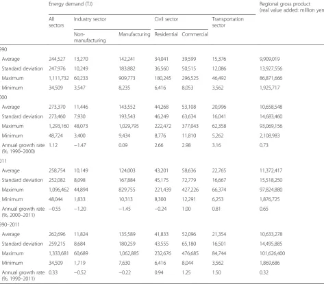
Table 1 summarizes the relevant data statistics for Japan. Comparing the average energy demand for each sector shows a constant high demand level in the manu-facturing sector. The average values for the civil sectors (residential and commercial) and the transportation sec-tor are relatively small in comparison. During the study
period (1990–2011), the manufacturing sector’s
max-imum energy demand was extremely large (1,029,795 TJ in 2000), and its minimum energy demand was very small (8235 TJ in 1990). In other words, there was a sig-nificant difference between the maximum and minimum values. Additionally, there was a large variation in the data for each prefecture.
In the 1990s, there was an increase in the average an-nual growth rate of energy demand in most sectors. En-ergy demand grew at 1.12 % for all sectors, at 0.09 % in the manufacturing sector, and at 2.98 % in the commer-cial sector. However, in the 2000s, the overall average growth rate fell to−0.55 %, driven mainly by a fall in the
manufacturing sector growth rate to −1.45 %.
Contrast-ingly, energy demand in the commercial and the trans-portation sector increased to 1.00 % and 0.81 %, respectively. These trends reflect the overall energy use trend at the time, namely a move from the manufactur-ing sector in the 1990s to the commercial sector throughout the 2000s. Looking at the absolute value of the change, the absolute amount of the energy demand reduction in the manufacturing sector is roughly equal to the increase in the energy demand in the commercial sector.
Japan’s average annual value-added growth rate
in-creased constantly in the 1990s and the 2000s. The growth rate trend represented by the value-added figures validates the energy intensity (energy demand per value added), namely a rapid drop from the 1990s to the 2000s.
Results and discussion Dynamic shift-share analysis
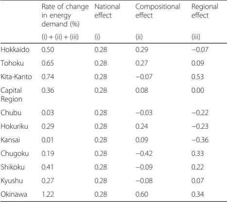
Table 2 gives the factor decomposition results for the
three effects on Japan’s regional energy demand using
However, in Hokkaido and Hokuriku, while the compos-itional effect contributed to an increase in energy de-mand, the regional effect’s contribution was negative. Conversely, in Japan’s western regions, such as Chugoku, Shikoku, and Kyushu, the regional effect’s contribution to the increase in energy demand was larger than that of the compositional effect. The lowering of the energy de-mand in the big-city regions (excluding the Capital
Re-gion), such as Chubu and Kansai, was affected
appreciably by the regional effects. Particularly, the con-tributions of the effects were negative for Chubu and Kansai. This reveals that in the big-city regions, the en-ergy demand fell via differences arising from regional-specific factors.
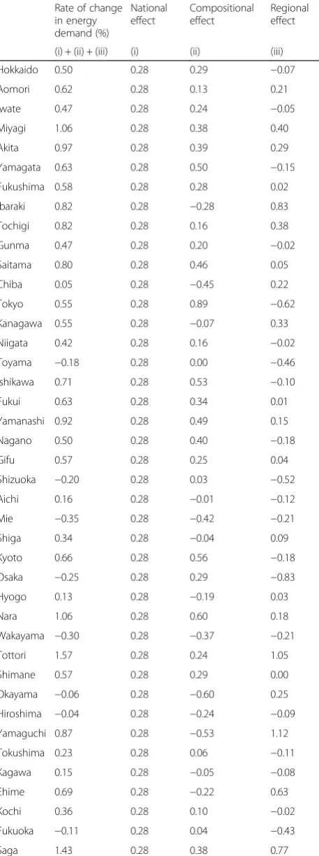
Table 3 gives the energy demand decomposition re-sults for Japan’s prefectures using dynamic shift-share
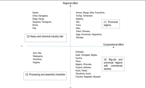
analysis. The energy demand increase exceeded 1 % in Miyagi, Nara, Tottori, Saga, Kumamoto, Kagoshima, and Okinawa prefectures. Conversely, the rate of change was negative in several prefectures, including Toyama, Shizu-oka, Mie, Osaka, Wakayama, Okayama, Hiroshima, and Fukuoka prefectures. A positive sign represents a posi-tive effect on the rate of change in energy demand. A negative sign represents a negative effect on the rate of change in energy demand. The national effect is positive but is not dominant. It is important to understand the characteristics of each prefecture, in relation to the re-gional differences arising from the compositional and the regional effects of energy demand. Hence, the pre-fectures were classified according to four quadrants, formed by the compositional effect on the horizontal axis and the regional effect on the vertical axis (Fig. 1). Table 1Japan’s energy demand by sector and real value added (1990–2011)
Energy demand (TJ) Regional gross product
(real value added: million yen)
All sectors
Industry sector Civil sector Transportation sector
Non-manufacturing
Manufacturing Residential Commercial
1990
Average 244,527 13,270 142,241 34,041 39,599 15,376 9,909,019
Standard deviation 247,976 10,249 183,882 36,560 50,515 12,086 13,927,556
Maximum 1,111,732 60,233 909,773 180,245 296,525 46,492 86,871,666
Minimum 34,509 3,547 8,235 6,416 8,053 3,562 1,925,717
2000
Average 273,370 11,446 143,552 44,268 53,108 20,996 10,658,548
Standard deviation 273,460 7,930 193,543 46,249 63,634 16,041 14,683,460
Maximum 1,293,160 48,073 1,029,795 222,472 377,043 62,358 93,069,156
Minimum 48,724 3,400 9,434 8,776 11,810 5,262 2,108,983
Annual growth rate (%, 1990–2000)
1.12 −1.47 0.09 2.66 2.98 3.16 0.73
2011
Average 258,754 10,149 124,003 43,201 58,636 22,765 11,372,417
Standard deviation 252,082 8,098 167,884 45,175 72,779 16,667 15,518,250
Maximum 1,096,462 44,894 829,755 221,439 427,226 66,374 97,824,880
Minimum 48,044 1,833 10,313 8,300 12,291 6,253 1,876,725
Annual growth rate (%, 2000–2011)
−0.55 −1.20 −1.45 −0.24 1.00 0.81 0.65
1990–2011
Average 262,696 11,824 135,589 41,833 52,096 21,354 10,633,278
Standard deviation 259,215 8,684 180,259 43,555 65,180 16,501 14,495,885
Maximum 1,333,681 60,689 1,062,885 232,676 476,685 84,744 101,626,400
Minimum 34,509 1,719 7,630 6,416 8,044 3,562 1,869,686
Annual growth rate (%, 1990–2011)
0.33 −0.52 −0.22 0.94 1.25 1.50 0.32
The compositional and the regional effects are both positive in the first quadrant: a characteristic of many of the prefectures that are not in big-city regions. In the second quadrant, the compositional effect is negative, and the regional effect is positive. Many of the provincial prefectures that have an agglomeration of heavy and chemical industries, which includes the petrochemical industrial complex, are in this quadrant. In the third quadrant, both the compositional and the regional ef-fects are negative. The prefectures of regions that have an agglomeration of processing and assembly industries are in this quadrant. In the fourth quadrant, the com-positional effect is positive and the regional effect is negative. Many prefectures that belong to the big-city re-gions with commercial sector agglomeration are in this quadrant. This quadrant also includes some provincial prefectures, such as Hokkaido, Toyama, Ishikawa, and Kochi.
These observations show that the positive/negative state of the compositional effect appears to be subject to the agglomeration degree of the manufacturing indus-tries. Further, the positive/negative state of the regional effect seems to be subject to whether the region is a big-city region or a provincial region.
Analysis of the compositional effect
The dynamic shift-share analysis shows a high correl-ation between the level of agglomercorrel-ation of the manu-facturing sector and the positive or negative state of the compositional effect. Therefore, it is worth investigating this relationship in more detail. The differences in the compositional effect among the prefectures depend on the users (industrial, civil, or transportation sectors) in each prefecture. Here, the article verifies which user has an effect on the compositional effect according to a loca-tion quotient showed by McCann [23]. A localoca-tion
quo-tient is usually calculated using the number of
employees. The article calculates this location quotient for energy demand. The location quotient (represented byLQ)of the energy demand of useriin regionjin time
tis given by
LQij;t¼Eij;t=Ej;t Ei;t=Et :
The numerator shows the energy demand share of useriin regionj. The denominator shows the energy de-mand share of user i for the entire nation. Accordingly, if the index exceeds one, then the region’s energy de-mand share of useriis higher than that of the entire na-tion. If the index exceeds one, then the region has a comparative agglomeration of that user.
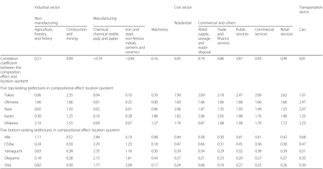
Table 4 gives the correlation coefficient between the compositional effect and the location quotient,
calcu-lated for 1990 (t= 1990). The results show a negative
trend for the compositional effect when a region special-izes in manufacturing, particularly for the chemical, chemical textile, and pulp and paper sectors, and the iron and steel, non-ferrous metal, and cement and cer-amics sectors. Meanwhile, the results also show a posi-tive trend for the compositional effect for regions that specialize in civil activities, such as the residential and commercial sectors and the transportation sector cen-tered on passenger vehicles.
The following observations are made from checking the location quotient of the energy demand by user for the five highest-ranking prefectures, and the five lowest-ranking prefectures, with respect to the rate of change by compositional effect. For the highest-ranking prefec-tures, the location quotient for the residential, commer-cial, and transportation sectors was more than one, and high. In contrast, the location quotient of the heavy and chemical industries (particularly the chemical, chemical textile, and pulp and paper industry, and the iron and steel, non-ferrous metal, and cement and ceramics in-dustry) is close to zero, and extremely low. For the low-est ranking prefectures, this relationship is reversed.
In other words, in prefectures that specialize in civil activities (including the residential and commercial Table 2Factor decomposition of energy demand by Japanese
region (1990–2011) Rate of change in energy demand (%)
National effect
Compositional effect
Regional effect
(i) + (ii) + (iii) (i) (ii) (iii)
Hokkaido 0.50 0.28 0.29 −0.07
Tohoku 0.65 0.28 0.27 0.09
Kita-Kanto 0.74 0.28 −0.07 0.53
Capital Region
0.36 0.28 0.08 0.00
Chubu 0.03 0.28 −0.03 −0.22
Hokuriku 0.29 0.28 0.24 −0.23
Kansai 0.01 0.28 0.09 −0.36
Chugoku 0.19 0.28 −0.42 0.33
Shikoku 0.41 0.28 −0.09 0.22
Kyushu 0.27 0.28 −0.08 0.07
Okinawa 1.22 0.28 0.60 0.34
Notes:
1. The rate of change is the annual average (%) for 1990–2011 2. The regions are broken down as follows:
Hokkaido (Hokkaido)
Tohoku (Aomori, Iwate, Miyagi, Akita, Yamagata, Fukushima, Niigata) Kita-Kanto (Ibaraki, Tochigi, Gunma, Yamanashi)
Capital Region (Saitama, Chiba, Tokyo, Kanagawa) Chubu (Nagano, Gifu, Shizuoka, Aichi, Mie) Hokuriku (Toyama, Ishikawa, Fukui)
Kansai (Shiga, Kyoto, Osaka, Hyogo, Nara, Wakayama) Chugoku (Tottori, Shimane, Okayama, Hiroshima, Yamaguchi) Shikoku (Tokushima, Kagawa, Ehime, Kochi)
sectors and the transportation sector), the rate of in-crease in energy demand is large. Meanwhile, in prefec-tures that specialize in heavy and chemical industries, a negative rate of change is observed for energy demand by way of the compositional effect.
Analysis of the regional effect
The differences in the compositional effect rely on dif-ferences in the specialization of the energy user of each prefecture. The differences in the regional effect rely on the differences in the regionally unique characteristics of each of the prefecture’s energy users. The results of dy-namic shift-share analysis show a high correlation be-tween the positive or negative state of the regional (big-city versus provincial regions) effect, and it is worth in-vestigating this relationship in greater detail. To gain a more detailed understanding, the portion of the regional effect∑isij[g(Eij)−g(Ei)] in (3) is resolved into the degree
of energy intensity and the real gross product (value added).3
First, the region’s energy consumption for each user can be resolved with approximate equations using the formula
g Eij ¼g Eij=Yj
þg Yj ; ð4Þ whereYjis the real gross product of region j, andEij/
Yjis the energy intensity of useri in regionj. Moreover,
the nation’s energy consumption for each user can be re-solved with approximate equations using the formula
g Eð Þ ¼i g Eð i=YÞ þg Yð Þ; ð5Þ where Yis the national gross product, and Ei/Y is the
national energy intensity for user i. Substituting (4) and (5) into the regional effect portion of (3) yields
X
isij g Eij −g Eð Þi
¼Xisij g Eij=Yj
−g Eð i=YÞ
þ g Yj −g Yð Þ
:
ð6Þ
The regional effect is expressed as the sum of the change of energy intensity and regional gross product, specifically, as follows.
Table 3Factor decomposition of Japan’s prefectural energy demand (1990–2011)
Rate of change in energy demand (%)
National effect
Compositional effect
Regional effect
(i) + (ii) + (iii) (i) (ii) (iii)
Hokkaido 0.50 0.28 0.29 −0.07
Aomori 0.62 0.28 0.13 0.21
Iwate 0.47 0.28 0.24 −0.05
Miyagi 1.06 0.28 0.38 0.40
Akita 0.97 0.28 0.39 0.29
Yamagata 0.63 0.28 0.50 −0.15
Fukushima 0.58 0.28 0.28 0.02
Ibaraki 0.82 0.28 −0.28 0.83
Tochigi 0.82 0.28 0.16 0.38
Gunma 0.47 0.28 0.20 −0.02
Saitama 0.80 0.28 0.46 0.05
Chiba 0.05 0.28 −0.45 0.22
Tokyo 0.55 0.28 0.89 −0.62
Kanagawa 0.55 0.28 −0.07 0.33
Niigata 0.42 0.28 0.16 −0.02
Toyama −0.18 0.28 0.00 −0.46
Ishikawa 0.71 0.28 0.53 −0.10
Fukui 0.63 0.28 0.34 0.01
Yamanashi 0.92 0.28 0.49 0.15
Nagano 0.50 0.28 0.40 −0.18
Gifu 0.57 0.28 0.25 0.04
Shizuoka −0.20 0.28 0.03 −0.52
Aichi 0.16 0.28 −0.01 −0.12
Mie −0.35 0.28 −0.42 −0.21
Shiga 0.34 0.28 −0.04 0.09
Kyoto 0.66 0.28 0.56 −0.18
Osaka −0.25 0.28 0.29 −0.83
Hyogo 0.13 0.28 −0.19 0.03
Nara 1.06 0.28 0.60 0.18
Wakayama −0.30 0.28 −0.37 −0.21
Tottori 1.57 0.28 0.24 1.05
Shimane 0.57 0.28 0.29 0.00
Okayama −0.06 0.28 −0.60 0.25
Hiroshima −0.04 0.28 −0.24 −0.09
Yamaguchi 0.87 0.28 −0.53 1.12
Tokushima 0.23 0.28 0.06 −0.11
Kagawa 0.15 0.28 −0.05 −0.08
Ehime 0.69 0.28 −0.22 0.63
Kochi 0.36 0.28 0.10 −0.02
Fukuoka −0.11 0.28 0.04 −0.43
Saga 1.43 0.28 0.38 0.77
Table 3Factor decomposition of Japan’s prefectural energy demand (1990–2011)(Continued)
Nagasaki 0.44 0.28 0.42 −0.26
Kumamoto 1.25 0.28 0.34 0.63
Oita 0.24 0.28 −0.61 0.57
Miyazaki 0.18 0.28 0.04 −0.14
Kagoshima 1.12 0.28 0.36 0.48
Okinawa 1.22 0.28 0.60 0.34
Energy-intensity effect:∑isij[g(Eij/Yj)−g(Ei/Y)]
Production effect: [g(Yj)−g(Y)]
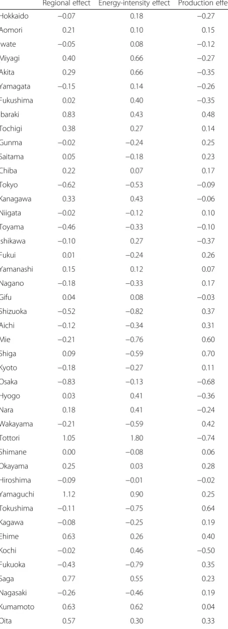
Table 5 gives the results of the decomposition using (6). The regional effect is not attributable to an energy user composition; therefore, it is difficult to discuss the regional effect contributions that give rise to energy in-tensity and production activity as a trend of the
compos-itional difference by user. Therefore, this paper
considers the breakdown of the factor analysis results for both the top-ranking and the bottom-ranking prefec-tures, in terms of the rate of change attributable to the regional effect.
The top-ranking prefectures in terms of the rate of change attributable to the regional effect are in provin-cial regions, i.e., Yamaguchi prefecture, followed by Tot-tori, Ibaraki, Saga, and Ehime prefectures. An observable characteristic of these regions is that, except for Tottori prefecture, both the energy-intensity and the production effects contribute positively. For the ten top-ranking pre-fectures, both of these factors contribute positively to the regional effect, and no notable differences in the size of this contribution are observed. Meanwhile, the bottom-ranking prefectures are those in the big-city re-gions, with Osaka at the very bottom, followed by Tokyo, Shizuoka, Toyama, and Fukuoka prefectures. An observable characteristic of these regions is that the energy-intensity effects are all negative. Moreover, there
is a tendency for the size of these effects to exceed the production effect. Therefore, it is highly possible that the rate of change in the regional effect is negative mainly owing to a declining energy-intensity effect. Note that the energy-intensity effect for the ten bottom-ranking prefectures is negative.
Accordingly, the obtained results suggest that it is pos-sible to explain the differences between big-city and pro-vincial regions, which are expressed as the regional differences of the regional effect, i.e., differences not in the production effect but in the energy-intensity effect. Last, the correlation coefficient between the regional ef-fect and the energy-intensity efef-fect is 0.76 and that be-tween the regional effect and the production effect is 0.08. This shows that the correlation coefficient between the regional effect and the energy-intensity effect is rela-tively high, compared with that between the regional ef-fect and production efef-fect.
Conclusions
To clarify what factors determine the fluctuations in the regional energy demand in Japan, this study applied dy-namic shift-share analysis to the fluctuations in regional energy demand. The results show that although there is a positive contribution from the national effect, it is not dominant. Further, the positive and the negative
Table 4Factor decomposition of the compositional effect in Japan, by sector and prefecture
Industrial sector Civil sector Transportation
sector
Non-manufacturing
Manufacturing
Residential Commercial and others
Agriculture, forestry, and fishery
Construction and mining
Chemical, chemical textile, pulp and paper
Iron and steel, non-ferrous metals, cement and ceramics
Machinery Water
supply, sewage and waste disposal
Trade and finance services
Public services
Commercial services
Retail services
Cars
Correlation coefficient between the composition effect and location quotient
0.21 0.89 −0.74 −0.69 0.16 0.95 0.79 0.86 0.87 0.93 0.94 0.81
Five top-ranking prefectures in compositional effect: location quotient
Tokyo 0.06 2.35 0.04 0.10 0.59 1.90 2.69 3.18 2.47 2.69 2.62 1.07
Okinawa 1.66 1.66 0.01 0.25 0.00 1.69 1.66 1.66 1.68 1.66 1.66 2.47
Nara 0.65 1.93 0.02 0.01 0.96 2.06 1.87 1.35 1.93 1.49 1.55 2.07
Kyoto 0.30 1.25 0.16 0.28 1.86 1.82 2.06 2.05 1.88 1.76 1.80 1.25
Ishikawa 2.14 1.55 0.09 0.07 1.27 1.74 0.87 1.68 1.48 1.70 1.72 2.23
Five bottom-ranking prefectures in compositional effect: location quotient
Mie 1.11 0.52 2.84 0.19 0.98 0.44 0.38 0.30 0.41 0.41 0.42 0.68
Chiba 0.24 0.50 2.29 1.25 0.18 0.47 0.66 0.31 0.45 0.36 0.36 0.47
Yamaguchi 0.63 0.38 2.35 1.16 0.30 0.39 0.34 0.29 0.32 0.38 0.39 0.51
Okayama 0.18 0.28 2.15 1.61 0.43 0.27 0.21 0.23 0.20 0.27 0.27 0.33
Oita 0.82 0.30 1.77 2.08 0.17 0.24 0.06 0.19 0.27 0.25 0.26 0.39
Notes: Location quotient is the value of 1990 (t= 1990)
Sustain
ability
and
Society
(2016) 6:10
Page
8
of
fluctuations in regional energy demands are determined by both the compositional and the regional effects.
The study found that the compositional effect contrib-utes most to energy demand growth in the prefectures that specialize in the civil and transportation sectors. Further, the compositional effect does not contribute to energy demand growth in the prefectures that specialize in the heavy and chemical industries of the manufactur-ing sector. Moreover, the study found that among the regional effects, the improvement in energy intensity through energy conservation (which is promoted mainly in big-city regions) contributes to constrain-ing the energy demand. For example, because of im-proved energy intensity, the energy demand declined in Mie, Wakayama, Osaka, Shizuoka, Toyama, Fuku-oka, and Hiroshima prefectures. That is, the regional effects in big-city regions are comparable and differ significantly from rural regions in terms of energy demand. This paper attributes this observation to the promotion of energy conservation in big-city re-gions. Future research could investigate the differ-ences between rural and urban areas in Japan that might prove to be causal to the statistical data used in this analysis.
The study concludes that the findings are reason-able, as the dynamic shift-share analysis focuses on the rate of change. The study expected that the
compositional effect—expressing the degree by which
the national energy demand from each energy user exceeds the rate of change of the national energy
demand—would be low in the manufacturing
indus-try, because energy demand changes mainly arise from efficiency efforts in this sector. The study also verifies that the agglomeration of industry enforces this effect (Otsuka et al. [5], Otsuka and Goto [6]). The study results are fully consistent with these insights.
The finding that the compositional and the re-gional effects are relevant to energy demand changes shows that having a mixture of industry and civil sector businesses in a region, potentially flattens out the fluctuations in energy demand changes. This suggests that when moderating the change of re-gional energy demand, it is important to diversify the industrial structure in each region. This finding should make an important contribution to planning Table 5Factor decomposition of the regional effect in Japan
Regional effect Energy-intensity effect Production effect
Hokkaido −0.07 0.18 −0.27
Aomori 0.21 0.10 0.15
Iwate −0.05 0.08 −0.12
Miyagi 0.40 0.66 −0.27
Akita 0.29 0.66 −0.35
Yamagata −0.15 0.14 −0.26
Fukushima 0.02 0.40 −0.35
Ibaraki 0.83 0.43 0.48
Tochigi 0.38 0.27 0.14
Gunma −0.02 −0.24 0.25
Saitama 0.05 −0.18 0.23
Chiba 0.22 0.07 0.17
Tokyo −0.62 −0.53 −0.09
Kanagawa 0.33 0.43 −0.06
Niigata −0.02 −0.12 0.10
Toyama −0.46 −0.33 −0.10
Ishikawa −0.10 0.27 −0.37
Fukui 0.01 −0.24 0.26
Yamanashi 0.15 0.12 0.07
Nagano −0.18 −0.33 0.17
Gifu 0.04 0.08 −0.03
Shizuoka −0.52 −0.82 0.37
Aichi −0.12 −0.34 0.31
Mie −0.21 −0.76 0.60
Shiga 0.09 −0.59 0.70
Kyoto −0.18 −0.27 0.11
Osaka −0.83 −0.13 −0.68
Hyogo 0.03 0.41 −0.36
Nara 0.18 0.41 −0.24
Wakayama −0.21 −0.59 0.42
Tottori 1.05 1.80 −0.74
Shimane 0.00 −0.08 0.06
Okayama 0.25 0.03 0.28
Hiroshima −0.09 −0.01 −0.02
Yamaguchi 1.12 0.90 0.25
Tokushima −0.11 −0.75 0.64
Kagawa −0.08 −0.25 0.19
Ehime 0.63 0.26 0.40
Kochi −0.02 0.46 −0.50
Fukuoka −0.43 −0.79 0.35
Saga 0.77 0.55 0.23
Nagasaki −0.26 −0.46 0.19
Kumamoto 0.63 0.62 0.04
Oita 0.57 0.30 0.33
Table 5Factor decomposition of the regional effect in Japan
(Continued)
Miyazaki −0.14 −0.43 0.27
Kagoshima 0.48 0.16 0.29
Japan’s national energy master plan. This result sug-gests that it is necessary to take into account the differences between the energy users and the regions to investigate the future trends of energy demand in Japan accurately.
Compared with static shift-share analysis, dynamic shift-share analysis accounts for the time variation of the industrial structure. In other words, dynamic shift-share analysis does not assume a time-fixed structure in energy demand, to enable the factor de-composition of continuous change in energy demand. That is, using dynamic shift-share analysis can allevi-ate a static shift-share analysis problem: the potential over- or under-estimation of the energy change rate. Therefore, when evaluating the fluctuations in energy demand, the Japanese Government should adopt a dy-namic approach to capture the fluctuation of energy demand in a continuous time change, rather than fix-ing the observation period in a two-point static ap-proach. However, to assess the dynamic structure on the energy demand in detail, it is necessary to further decompose the regional differences in the energy de-mand by the energy user. This is a topic for future research on energy demand forecasting.
Endnotes 1
The energy demand drivers are also related to other issues, such as sociology (household size development, income-related luxury demands), technological advance-ment, or climate policies. However, to precisely investi-gate the impact of such issues on changes in energy demand requires an econometric analysis rather than a shift-share analysis. This is because shift-share analysis is only one of the decomposition methods (Metcalf [3]).
2
The dynamic approach is a suitable way to address the question of the representational adequacy of a continuous time in discrete models (Mitchell [20]).
3
There is a method of dividing to identify the finer factors. However, the calculation becomes inflation. This paper is simplified to the two factors that seem dominant.
Competing interests
The author declares that he has no competing interests.
Author’s contributions
The author conducted the analysis and drafted the manuscript.
Author’s information
Dr. Otsuka is an associate professor at the Yokohama City University, Japan.
Acknowledgements
The author is grateful to anonymous reviewers for their helpful comments and suggestions.
Funding
This work was supported by a Japan Society for the Promotion of Science (JSPS) Grant-in-Aid for Scientific Research (KAKENHI) 15K17067.
Received: 21 September 2015 Accepted: 27 March 2016
References
1. Ministry of Economy, Trade and Industry (METI), Agency for Natural Resources and Energy (2015) Outline of the FY2014 Annual Report on Energy (Energy White Paper 2015). http://www.meti.go.jp/english/report/ downloadfiles/2015_outline.pdf. Accessed 16 Mar 2016.
2. Bernstein MA, Fonkych K, Loeb S, Loughran DS (2003) State-level changes in energy intensity and their national implications., Rand Corp 3. Metcalf GE (2008) An empirical analysis of energy intensity and its
determinants at the state level. Energ J 29(3):1–26
4. Raupach-Sumiya J, Matsubara H, Prahl A, Aretz A, Salecki S (2015) Regional economic effects of renewable energies–comparing Germany and Japan. Energ Sustain Soc 5(1):1–17. doi:10.1186/s13705-015-0036-x 5. Otsuka A, Goto M, Sueyoshi T (2014) Energy efficiency and
agglomeration economies: the case of Japanese manufacturing industries. Reg Sci Pol Pract 6(2):195–212
6. Otsuka A, Goto M (2015) Estimation and determinants of energy efficiency in Japanese regional economies. Reg Sci Pol Pract 7(2):89–101 7. Dunn ES (1960) A statistical and analytical technique for regional
analysis. Pap Reg Sci 6(1):97–112
8. Dinc M, Haynes KE (1999) Source of regional inefficiency: an integrated shift-share, data envelopment analysis and input-output approach. Ann Regional Sci 33(4):469–489
9. Haynes KE, Dinc M (1997) Productivity change in manufacturing regions: a multifactor/shift-share approach.
Growth Change 28(2):201–221
10. Dawson JA (1982) Shift-share analysis: a bibliographic review of technique and applications. (No. 949). Vance Bibliographies, Monticello
11. Knudsen DC, Barff RA (1991) Shift-share analysis as a linear model. Environ Plann A 23(3):421–431
12. Artige L, Neuss LV (2014) A new shift-share method. Growth Change 45(4):667–683
13. Barff RA, Knight PL III (1988) Dynamic shift-share analysis. Growth Change 19(2):1–10
14. Esteban-Marquillas JM (1972) A reinterpretation of shift-share analysis. Reg Urban Econ 2(3):249–255
15. Haynes KE, Machunda ZB (1987) Considerations in extending shift-share analysis: note. Growth Change 18(2):69–78
16. Markusen AR, Nooponen H, Driessen K (1991) International trade, productivity, and US regional job growth: a shift-share interpretation. Int Reg Sci Rev 14(1):15–39
17. Marquez MA, Ramajo J, Hewings GJD (2009) Incorporating sectoral structure into shift–share analysis. Growth Change 40(4):594–618
18. Hirobe T (2015) Economic shift-share effects and spatial agglomeration regarding inter-regional disparities of labour market in the USA. Reg Sci Pol Prac 7(3):103–117
19. Kobayashi N (2004) Industrial structure and manufacturing growth during Japan’s bubble and post-bubble economics.
Reg Stud 38(4):429–444
20. Mitchell W, Carlson E (2005) Exploring employment growth disparities across metropolitan and regional Australia. Austral J Reg Stud 11(1):25–40
21. Nissan E, Carter G (1994) An extension to the shift-share technique for predicting and evaluating changes in employment growth. J Reg Anal Pol 24(2):49–67
22. Shi C, Zhang J, Yang Y, Zhang Z (2007) Shift-share analysis on international tourism competitiveness: a case of Jiangsu province. Chinese Geogr Sci 17(2):173–178