© Author(s) 2008. This work is distributed under the Creative Commons Attribution 3.0 License.
Snow melting bias in microwave mapping of Antarctic snow
accumulation
O. Magand, G. Picard, L. Brucker, M. Fily, and C. Genthon
Laboratoire de Glaciologie et G´eophysique de l’Environnement, CNRS, Universit´e Joseph Fourier-Grenoble, 54 Rue Moli`ere, BP 96, 38402 St Martin d’H`eres Cedex, France
Received: 13 February 2008 – Published in The Cryosphere Discuss.: 24 April 2008 Revised: 29 August 2008 – Accepted: 29 August 2008 – Published: 12 September 2008
Abstract. Satellite records of microwave surface emission have been used to interpolate in-situ observations of Antarc-tic surface mass balance (SMB) and build continental-scale maps of accumulation. Using a carefully screened subset of SMB measurements in the 90◦–180◦E sector, we show a reasonable agreement with microwave-based accumulation map in the dry-snow regions, but large discrepancies in the coastal regions where melt occurs during summer. Using an emission microwave model, we explain the failure of mi-crowave sensors to retrieve SMB by the presence of lay-ers created by melt/refreeze cycles. We conclude that re-gions potentially affected by melting should be masked-out in microwave-based interpolation schemes.
1 Introduction
Arthern et al., 2006 have recently produced a new Antarctic Surface Mass Balance (SMB) map (referred as A06) using both field measurements and microwave and thermal infrared remote sensing data. The same SMB measurements as in the former SMB map (Vaughan et al., 1999) (referred as V99) are used, but a new geostatistical method is applied to inter-polate the ground measurements to every point of the gridded map. The interpolation relies on a spatial background model of the accumulation based on the annual-mean thermal in-frared temperature and the polarisation ratio of microwave brightness temperature at 4.3 cm wavelength (6.9 GHz). Mi-crowave brightness temperature has been shown to be a good proxy of SMB in Greenland (Winebrenner et al., 2001) and in Antarctica (Vaughan et al., 1999). These former studies used however a shorter wavelength (0.8 cm, i.e. 37 GHz) which is more sensitive to snow grain scattering and consequently
Correspondence to: G. Picard
(ghislain.picard@lgge.obs.ujf-grenoble.fr)
is more dependent on grain size. According to A06, the new map describes the average SMB with an accuracy of 10% or better at an effective spatial resolution of 100 km. The au-thors also suggest the new SMB map may eliminate some of the discrepancies between climate models and earlier compi-lations or maps of SMB as observed by (Genthon and Krin-ner, 2001).
5 10 15 20 25 30
90˚
120˚
150˚
180˚
−85˚
−85˚
−80˚
−80˚
−75˚
−75˚
−70˚
−70˚
−65˚
−65˚
−60˚
−60˚
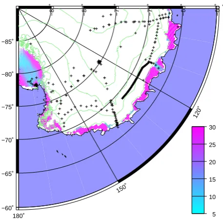
Fig. 1. Area of investigation with distribution pattern of surface
melting areas observed in 90–180◦ East Antarctica sector, from
1979 to 2006, by the SMMR (1979–1988) and SSM/I (1988– onward) microwave radiometers. Crosses represent the filtered ob-served SMB data resulting from M07. Melting areas are expressed in average melting days by year.
more detail the effect of melting on the SMB retrieval and show that even moderate or rare melting, covering a signifi-cant surface of the Antarctic, degrades the retrieval.
In this paper, we concentrate in the 90◦–180◦E sector. Quality-controlled and updated SMB observations (referred as M07) (Magand et al., 2007) confirm the good accuracy of A06’s map in ever-dry-snow region as on the Antarctic Plateau (Sect. 3.1) but also show the negative impact of sur-face melting (Sect. 3.2). With physical arguments and by using a physical microwave emission model (Sect. 4) we ex-plain and evaluate quantitatively the effect of surface melting on the polarisation ratio. Section 5 gives conclusions and recommendations.
2 Data and methods
2.1 Selection of observed SMB data in 90◦–180◦E sector Recently, (Magand et al., 2007) produced a quality-controlled dataset of SMB measurements by discarding SMB measurements which do not fit quality criteria based on 1) an up-to-date review and quality rating of various SMB mea-surement methods and 2) coherency, completion, or lack of meta-information (location, date of measurement, time pe-riod covered by the SMB values, primary data sources) re-lated to each SMB record. The filtering procedure was ap-plied on V99‘s dataset (the same data are also in A06) in
Table 1. Mean relative differences (±1σ )between various interpo-lated A06 SMB data set at M07 site measurements. Different inter-polation methods are Nearest Grid Point (A06-NGP) and average of values within a radius of 20 (A06-20), 50 (A06-50) and 100 km (A06-100). In parenthesis, the maximum relative difference value.
A06-20 km A06-50 km A06-100 km
A06-NGP 2±2% (15%) 3±4% (32%) 5±6% (63%)
A06-20 km – 2±3% (19%) 4±5% (47%)
A06-50 km – 3±2% (24%)
the 90◦–180◦E Antarctic sector, from Queen Mary to Victo-ria Lands (Fig. 1). New SMB measurements from the Aus-tralian, Russian and Italian-French scientific activities since 1998 (see references in Magand et al., 2007) have been added and provide independent ground-truth as they were not used by A06. A high quality dataset is thus obtained at the cost of a strong reduction in observation number and spatial cov-erage. In the present work, A06’s interpolated SMB data are compared to our quality controlled dataset.
2.2 Comparison method
Each M07 measurement (corresponding to a field point) is compared to the nearest A06 grid-point (NearestGP) value, as well as to the average of A06’s SMB values within a ra-dius of 20, 50 and 100 km to prevent representativeness mis-interpretation.
Relative differences are calculated as follows: Rel.Diff.= A06i −A06j
A06i
!
×100 (1)
with A06i,j, the interpolated A06’s SMB value at
resolu-tioniandj, and associated to each observed SMB data. Ta-ble 1 shows relative differences between different methods are small.
The highest disagreement (mean value of 5±6%) is ob-served between the nearest grid-point method and the aver-age within 100 km (A06-100). Since the difference is small, only the average values within 100 km are presented in the next sections. Other dataset (NearestGP, 20 km, 50 km) were also used but no major differences were found and conclu-sions are the same.
3 Results
3.1 A06-100 SMB versus M07 SMB
Table 2. Comparison between A06-100’s interpolated SMB data and different selections of corresponding observed SMB data (M07).
a“Outliers” are discarded from the present statistics.
bPF represent SMB data localized in areas characterized by Percolation Facies regions. RMS differences are expressed in kg m−2yr−1
(i.e. mm WE), and relative RMS are normalized by the A06-100 interpolated values.
M07 (V99)a M07 (new)a M07 (all)a M07 in PF areasb M07 minus PFb
RMS difference (kg m−2 yr−1) 85 58 77 126 61
Relative RMS difference (%) 31 46 35 51 28
n data 189 92 281 52 229
is good, demonstrating the quality of the A06’s SMB map in the studied sector. Larger scatter is found for the high-est accumulation rates, usually in coastal areas. At a first glance, this is not surprising because of the low spatial sam-pling density in the latter areas characterized by high natural variability of the net accumulation.
Most points fit in the range of normally distributed y-residuals from the regression line. Only two points (not shown in the figure) are clearly outside the main cloud of points. These outliers come from an area between the Law Dome saddle (67◦150S, 112◦E) at 800 m a.s.l. and A028 (68◦240S, 112◦E) at 1650 m a.s.l. (Goodwin, 1988). Mea-sured SMB is twice higher (781 and 806 kg m−2yr−1)than in A06’s map (361 and 402 kg m−2yr−1, respectively). This is not surprising since the Law Dome region is characterized by strong precipitation, and SMB gradients due to the topog-raphy (Goodwin, 199; Goodwin et al., 2003). The typical length scale of elevation and spatial SMB variability is about 10 km (Van de Berg et al., 2006). The present-day SMB at Law Dome is marked by a very sharp east-west gradient; high accumulation on the east side is the result of dominant cyclonic flow from the south-east and the orographic effect of the dome (Van Ommen et al., 2004). Due to the large SMB gradients occurring in such small area, the 100 km resolu-tion A06’s SMB map may hardly be consistent with the local SMB observations. These two outliers are then discarded from our analysis and in particular the statistics (Table 2).
First column in Table 2 shows comparison between A06-100 and filtered V99 SMB data (i.e. a quality-controlled sub-set of data available to and used by A06). Relative RMS difference (31%) is in agreement with the error estimated by A06. Comparison with the new measurements (not used by A06) shows a larger RMS difference (46%; Table 2, column 2). Statistics for M07 (new data+V99) (Table 2, column 3) only slightly deteriorates the correlation with RMS differ-ence of 35% instead of 31%.
Looking at the altitudinal distribution of all SMB data from the coast to 4000 m a.s.l., we observe that:
Fig. 2. Comparison between observed SMB values from filtered
observed SMB data set (M07) to interpolated SMB values averaged at 100 km resolution (A06-100). Empty crosses correspond to ob-served SMB data used by V99 and A06, and black crosses represent new observed SMB data obtained from ITASE, RAE and ANARE projects since 1998 (see M07).
– New data are predominantly from the Antarctic plateau, above 2000 m a.s.l;
– A06’s map tends to over-estimate observed SMB val-ues on the Antarctic plateau, and under-estimate those below 2000 m a.s.l..
Fig. 3. Comparison between observed SMB values from filtered
observational SMB data sets (M07) to interpolated SMB values av-eraged in 100 km resolution (A06-100) with distribution pattern of
observed SMB points located inPercolationFacies (P F∼melting
events) areas. Cumulative melting days are calculated on the
ba-sis of 6.9 GHz microwave penetration depth (dp)of 10 m in snow
pack. SMB values are expressed in kg m−2yr−1(i.e. mm W.E.).
3.2 Snow melting areas and microwave signature
The presence of liquid water in snow induces a large in-crease of the emissivity and radical shortening of the pen-etration depth (Rott and Sturm, 1991) with respect to dry snow. This singular signature makes surface melting easily detectable by passive microwave remote sensing. Using 19 GHz horizontally polarised brightness temperature acquired by the SMMR (1979–1988) and SSM/I (1988–onward) mi-crowave radiometers, melt events are mapped every day (or every other day for SMMR) in Antarctica at about 50 km effective resolution (Torinesi et al., 2003; Picard and Fily, 2006). It is worth noting at this point that
– The dataset of melt events is independent of the mi-crowave observations used by A06 to produce the SMB map. Different microwave frequencies and time peri-ods are used (events detection uses daily data while the polarization ratio is based on many years average). – The technique does not provide information about the
amount of melted water during the event nor about the processes that occurs during and after the melt event (percolation, refreezing and so on) (but an improved method has been proposed recently for the Greenland Ice Sheet – Winebrenner et al., 2001). It is difficult to assess what happens during refreezing and whether
Fig. 4. Comparison between the logarithmically transformed
Polar-isation ratios issued from 2002–2006 satellite record and the M07
SMB values. Polarisation ratio is expressed asPminus component
P0; this last component of polarization being issued from reflection
at the air-snow interface as thermal emission leaves the snow. Ob-served SMB data located in Percolation Facies areas are reported. Cumulative melting days are calculated on the basis of 6.9 GHz
mi-crowave penetration depth (dp)of 10 m in snow pack.
a dense or ice layer is formed. As a consequence, the number of melt events is only a rough proxy for the number of ice layers.
The number of ice layers that could affect the polarisation ratio at 6.9 Ghz depends on the number of melt events that have occurred in the past, the microwave penetration depth and the accumulation which governs burial of ice layers. At 6.9 GHz, observed brightness temperature results from the emission in the upper tens of meters (Surdyk, 1995; Surdyk, 2002). Penetration depth at 5.3 GHz is also estimated of the order of tens of meters in dry polar firn (Partington, 1998; Bingham and Drinkwater, 2000). Depending on the annual SMB, dense layers in the first tens of meters have formed a few years up to decades ago. To estimate the number of melt layers in the 10 first meters, we computed the total number of melting days during the period required for accumulating such quantities of snow. A mean snow density of 500 kg m−3
is assumed.
from the wet-zone are clearly divided in two groups depend-ing on the number of meltdepend-ing days (Fig. 3). The horizontal alignment for each group shows the absence of relationship between A06-100 SMB and the field observations. This re-sults in a larger RMS difference (51% instead of 34% with all data, Table 2, column 4). The RMS difference is even larger (56%) if only points affected by more than 10 melting days are considered.
4 Discussion
From Table 2 it is clear that excluding SMB data from melt zones clearly improves the fit between A06 map and the ob-servations with RMS relative difference of 28% instead of 35%. We further investigate here the physical origin of this result. The polarisation ratio is sensitive to the number of lay-ers and density contrast between these laylay-ers. Large polarisa-tion ratio corresponds to strong stratificapolarisa-tion. Any change of density in the snowpack as well as the top air-snow interface are seen by microwaves as a change in refractive index. At observation angles around 50◦–53◦close to the Brewster an-gle, every interface preferentially transmits vertically polar-ized waves and, equivalently, preferentially reflects horizon-tally polarized waves (West et al., 1996). The microwaves emitted by thermal agitation in the deep layers of the snow pack must cross many interfaces before escaping from the snow pack and reaching the satellite. Since the transmission at each interface is larger for the vertically-polarized wave, the brightness temperature at vertical polarisation is larger than the horizontally one, and the difference between both polarisations increases with the number of layers and density contrast. The polarisation ratioP−P0is then proportional to
the layer number within the snow-pack, whereP0=0.035 is
the polarisation ratio due to the air-snow interface (Arthern et al., 2006):
P =TB(V )−TB(H )
TB(V )+TB(H )
(2) The link between number of layers and accumulation is less clear. Winebrenner et al., 2001 related the variation in polari-sation ratios (modelling and in situ observations) to the accu-mulation occurring at different observation points in Green-land dry snow region. They showed a strong link between random firn density contrast variations and the SMB. Arthern et al., 2006 extended this approach by accounting for a tem-perature dependence on the stratification kinetic in Antarc-tica (layers form slower at lower temperature). Further inves-tigations are needed to understand the link between accumu-lation and stratification but from a pragmatic point of view, a clear relationship exists and allows accurate SMB estimation in dry zones.
In the melt areas, the polarisation ratio is not so clearly related to the accumulation. Figure 4 showsLn(P−P0)as
a function ofLn(M07 SMB). Similarly to A06, brightness
temperature (Tb) at 6.9 Ghz acquired by the Advanced
Mi-crowave Scanning Radiometer (ASMR-E) on Aqua satellite (Cavalieri, 2004) are averaged between 2002 and 2006 and used to estimate the polarisation ratioP−P0. The overall
correlation is significantly different from zero at the 99% level (n=278; R=0.708; p<0.01). However, distinguishing points between dry and melt zones shows a) that most of the points located in melt zones are characterized by higher po-larisation ratio than those with similar SMB in the dry zones and b) there is no clear dependence between the SMB values in melt zones and the polarisation ratio. The SMB thus can-not be directly correlated to the polarisation ratio. By elimi-nating points affected by melting, the relationship between polarisation ratio and SMB is stronger (n=227; R=0,850;
p<0.01).
Using the Microwave Emission Model of Layered Snow packs (Wiesmann and M¨atzler, 1999), we have simulated the polarisation ratioP−Pofor a variety of structured snow
packs. We found that a snow pack composed of snow layers (fine grain, density 400 kg m−3)interleaved with 3-cm thick ice layers (density 700 kg m−3)regularly spaced every 2 m has a polarisation ratio ofLn(P−Po)=–2.0, the upper bound
of those observed in Fig. 4 for the pixels in the melt areas. A single melt event every 2 years is sufficient for creating such a structure assuming 1-m annual accumulation. More ice lay-ers or weaker accumulation would lead to larger polarisation ratio. These results show that even infrequent melt events result in polarisation ratios larger than the typical range of polarisation used to retrieve SMB. It means that even infre-quent melting disrupts significantly the relationship between
P−Poand SMB.
5 Conclusions
Comparing the recent A06’s Antarctic SMB map with quality-controlled in-situ observations in the 90◦–180◦East Antarctic sector (Magand et al., 2007), we show that, in spite of a fair overall agreement on the plateau, there is a poor agreement in the coastal regions affected by surface melting, even infrequent. The disagreement in melt areas is a con-sequence of the fact that melt-refreeze layers affect the mi-crowave emissivity in horizontal polarisation more strongly than accumulation does. In some other places, the polarisa-tion ratio may even be unrelated to the SMB. This includes the blue ice area (Bintaja, 1999; Winther et al., 2001) where no snowpack layering is present, and the megadune areas. The morphology of megadunes is complex (Frezzotti et al., 2002) but the snowpack seems to be weakly structured as revealed by the lower polarisation ratio (around 0.05 in the megadune field South of Dome C) than in the surrounding (around 0.07) or on the ice divide (around 0.09). Since a low polarisation ratio is interpreted as an high accumulation, it is not surprising that A06 map shows larger accumulation in the megadune field South of Dome C than around although the accumulation is probably lower there (Courville et al., 2007). Further statistical analysis is however difficult given the lack of in situ SMB measurements in these areas.
Surface melting in the 90–180◦E sector in East Antarctica observed by microwave radiometers (Picard and Fily, 2006) represents more than 0.6×10⁶km2 i.e. approximately 14% of the sector (∼4.4×10⁶km2). Because the mean SMB is comparatively higher in the coastal zones, the mean SMB in the melt areas is∼24% of total SMB in the sector. Extrapo-lating to the whole of Antarctica, melt areas represent∼25% of the total surface and about 42% of the total SMB. Areas affected by surface melting are then far from negligible in terms of surface area and even less so in terms of accumula-tion volume. Thus, while A06 provides the latest and most up-to-date evaluation of the spatial distribution of SMB over Antarctica, along with an original and useful evaluation of er-rors, it is expected that not using microwave observations in melt areas for building the background model could further increase the accuracy of the map.
Acknowledgements. In Wilkes and Victoria Land sectors, most of
observed Surface Mass Balance data were obtained from recent research carried out in the framework of the Italian PNRA in collaboration with ENEA Roma, and supported by the French Polar Institute (IPEV). The authors are grateful to all colleagues who participated in field work and sampling operations and those whose comments and editing helped to improve the manuscript.
Edited by: M. Van den Broeke
References
Arthern, R. J., Winebrenner, D. P., and Vaughan, D. G.: Antarctic snow accumulation mapped using polarisation of 4.3cm wave-length microwave emission, J. Geophys. Res., 111, D06107, doi:10.1029/2004JD005667, 2006.
Bingham, A. W. and Drinkwater, M.: Recent changes in the mi-crowave scattering properties of the Antarctic ice sheet, IEEE Transactions on Geoscience and Remote Sensing, 38, 1810– 1820, 2000.
Cavalieri, D. and Comiso, J.: AMSR-E/Aqua daily L3 25 km Tb, sea ice temperature and sea ice conc, polar grids V001, January to December 2003., Natl. Snow and Ice Data Cent., Boulder, Col-orado, 2004.
Drinkwater, M. R., Long, D. G., and Bingham, A. W.: Greenland snow accumulation estimates from satellite radar scatterometer data, J. Geophys. Res., 106(D24), 33 935–33 950, 2001. Forster, R., Jezek, K. C., Bolzan, J., Baumgartner, F., and
Gogi-neni, P.: Relationships between radar backscatter and accumula-tion rates on the Greenland ice sheet, Int. J. Remote Sens., 20, 3131–3147, 1999.
Genthon, C. and Krinner, G.: Antarctic surface mass balance and systematic biases in general circulation models, J. Geophys. Res., 106, 20 653–20 664, 2001.
Goodwin, I. D.: Ice sheet topography and surface characteristics in Eastern Wilkes Land, East Antarctica, ANARE Research Notes, 64, 100 pp., 1988.
Goodwin, I. D.: Snow accumulation variability from seasonal surface observations and firn-core stratigraphy, Eastern Wilkes Land, Antarctica, J. Glaciol., 37, 383–387, 1991.
Goodwin, I. D., De Angelis, M., Pook, M., and Young, N. W.: Snow accumulation variability in Wilkes Land, East Antarctica, and the
relationship to atmospheric ridging in the 130◦–170◦E region
since 1930, J. Geophys. Res., 108, 4673–4689, 2003.
Magand, O., Genthon, C., Fily, M., Krinner, G., Picard, G., Frez-zotti, M., and Ekaykin, A. A.: An up-to-date quality-controlled
surface mass balance data set for the 90◦–180◦E Antarctica
sector and 1950–2005 period, J. Geophys. Res., 112, D12106, doi:10.1029/2006JD007691, 2007.
Munk, J., Jezek, K. C., Forster, R., and Gogineni, P.: An ac-cumulation map for the Greenland dry-snow facies derived from spaceborne radar, J. Geophys. Res., 108(D09), 4280, doi:10.1029/2002JD002481, ACL 8 1–12, 2003.
Partington, K. C.: Discrimination of glacier facies using multi-temporal SAR data, J. Glaciol., 44, 42–53, 1998.
Picard, G. and Fily, M.: Surface melting observations in Antarctica by microwave radiometers: Correcting 26-year time series from changes in acquisition hours, Remote Sens. Environ., 104, 325– 336, doi:10.1016/j.rse.2006.05.010, 2006.
Rott, H. and Sturm, K.: Microwave signature measurements of Antarctic and Alpine snow, In 11th EARSeL symposium, Graz, Austria, 140–151, 1991.
Surdyk, S.: Using microwave brightness temperature to detect short-term surface air temperature changes in Antarctica: An an-alytical approach, Remote Sens. Environ., 80, 256–271, 2002. Surdyk, S. and Fily, M.: Results of a stratified snow emissivity
model based on the wave approach: Application to the Antarctic ice sheet, J. Geophys. Res., 100, 8837–8848, 1995.
microwave sensors., J. Clim., 16, 1047–1060, 2003.
Van de Berg, W. J., Van den Broeke, M. R., Reijmer, C. H., and Van Meijgaard, E.: Reassessment of the Antarctic sur-face mass balance using calibrated output of a regional at-mospheric climate model, J. Geophys. Res., 111, D11104, doi:10.1029/2005JD006495, 2006.
Van den Broeke, M., Jan Van de Berg, W., Van Meijgaard, E., and Reijmer, C.: Identification of Antarctic ablation areas us-ing a regional atmospheric climate model, J. Geophys. Res., 111, D18110, doi:10.1029/2006JD007127, 2006.
Vaughan, D. V., Bamber, J. L., Giovinetto, M., Russell, J., and Cooper, A. P. R.: Reassessment of Net Surface Mass Balance in Antarctica, J. Clim., 12, 933–946, 1999.
West, R. D., Winebrenner, D. P., Tsang, L., and Rott, H.: Mi-crowave emission from density-stratified Antarctic firn at 6cm wavelength, Journal of Glaciology, 42, 63–76, 1996.