www.atmos-meas-tech.net/4/683/2011/ doi:10.5194/amt-4-683-2011
© Author(s) 2011. CC Attribution 3.0 License.
Measurement
Techniques
Retrieval of macrophysical cloud parameters from MIPAS:
algorithm description
J. Hurley, A. Dudhia, and R. G. Grainger
Atmospheric, Oceanic and Planetary Physics, Clarendon Laboratory, Department of Physics, Parks Road, Oxford, UK Received: 16 August 2010 – Published in Atmos. Meas. Tech. Discuss.: 26 August 2010
Revised: 29 March 2011 – Accepted: 3 April 2011 – Published: 7 April 2011
Abstract. The Michelson Interferometer for Passive Atmo-spheric Sounding (MIPAS) onboard ENVISAT has the po-tential to be particularly useful for studying high, thin clouds, which have been difficult to observe in the past. This pa-per details the development, implementation and testing of an optimal-estimation-type retrieval for three macrophysical cloud parameters (cloud top height, cloud top temperature and cloud extinction coefficient) from infrared spectra mea-sured by MIPAS. A preliminary estimation of a parameteri-sation of the optical and geometrical filling of the measure-ment field-of-view by cloud is employed as the first step of the retrieval process to improve the choice of a priori for the macrophysical parameters themselves.
Preliminary application to single-scattering simulations indicates that the retrieval error stemming from uncertainties introduced by noise and by a priori variances in the retrieval process itself is small – although it should be noted that these retrieval errors do not include the significant errors stemming from the assumption of homogeneity and the non-scattering nature of the forward model. Such errors are preliminarily and qualitatively assessed here, and are likely to be the dom-inant error sources. The retrieval converges for 99% of input cases, although sometimes fails to converge for vetically-thin (<1 km) clouds. The retrieval algorithm is applied to MIPAS data; the results of which are qualitatively compared with CALIPSO cloud top heights and PARASOL cloud opacities. From comparison with CALIPSO cloud products, it must be noted that the cloud detection method used in this algorithm appears to potentially misdetect stratospheric aerosol layers as cloud.
This algorithm has been adopted by the European Space Agency’s “MIPclouds” project.
Correspondence to: J. Hurley ([email protected])
1 Introduction
Although much of atmospheric infrared remote sensing is based upon analysis of data to estimate constituent concen-trations – where the presence of cloud particles in the mea-surements is treated as a source of error – it is possible to iso-late measurements of cloud in order to determine the proper-ties of clouds themselves. Clouds (especially high cloud such as cirrus) represent one of the largest uncertainties in climate studies (Intergovernmental Panel on Climate Change, 2008) – and in order to have reliable estimates of radiative forcing and climatic impact, accurate distributions of cloud frequen-cies and properties must be available. Satellite instruments provide an opportunity to study the properties of clouds on a global scale.
1.1 Overview of MIPAS-ENVISAT
The Michelson Interferometer for Passive Atmospheric Sounding (MIPAS) is an infrared limb-viewing instrument and was launched in March 2002 on the European Space Agency’s Environmental Satellite (ENVISAT). The polar or-bit of ENVISAT has large inclination, and enables global coverage pole-to-pole over a period of days, with an orbital repeat period of 35 days (European Space Agency, 2005).
1.5 km upward from approximately 4.5 km in the troposphere through the lower stratosphere (Mantovani, 2005). The MI-PAS field-of-view is trapezoidal in the vertical, with a verti-cal extent varying between 3–4 km, depending upon defini-tion. It has a characteristically wide horizontal field-of-view, extending approximately 200 km along the line-of-sight. 1.2 Overview of clouds from satellites
In this section, a very brief overview of the types of param-eters which are typically used to describe clouds is given, along with a sampling of general characteristics of different instruments which demonstrate how certain types of obser-vations are suitable for analysis of certain cloud properties (Sect. 1.2.1). Section 1.2.2 gives details of how instruments such as MIPAS tend to retrieve cloud properties.
1.2.1 Generalities of cloud measurement
Cloud properties fall loosely into two categories: macrophys-ical and microphysmacrophys-ical. Macrophysmacrophys-ical properties are the large-scale properties (i.e. bulk or extent), such as the alti-tude of a cloud, the physical depth and extent of a cloud, or are basic thermodynamic quantities, such as the temperature at the cloud top or the temperature structure within the cloud body. Microphysical parameters are, by opposition, those which relate to the small-scale of the cloud – such as the size and shape of cloud particles, and their distribution (which is often described in terms of water content), thus includ-ing properties such as number density, and influencinclud-ing cloud optical depth, albedo, emissivity and transmissivity. Cloud extinction is strictly a combination of macrophysical and mi-crophysical parameters as it is derived from both the physical extent of the cloud, as well as its absorption and scattering characteristics. However, for a model whereby there is no scattering, and a single homogeneous extinction characteris-ing the bulk of the cloud mass, as is the case in this study, the extinction coefficient is designated as a macrophysical parameter.
Most of our knowledge on the microphysical properties of clouds come from in-situ measurements: predominantly by aircraft-mounted instruments. Satellite instruments are par-ticularly well-suited to observing bulk cloud properties, such as average cloud top height and temperature, not least be-cause of the large-scale geographical regions they survey.
As a general rule, limb-viewing instruments are compe-tent at retrieving vertically-dependent parameters (such as cloud top height/pressure or cloud depth/extent) with great accuracy, although have poorer horizontal-resolving poten-tial. They are able to detect even clouds having thin opacities of less than 0.01 due to the inherently long limb pathlength. On the contrary, traditional nadir-viewing instruments gener-ally suffer from poor vertical resolution when retrieving at-mospheric temperature and composition from which cloud top temperatures (and hence cloud top heights/pressures) are
derived, and are limited to thicker clouds, but have very good horizontal resolution. It should be emphasized that nadir in-struments have a distinct advantage over their limb-viewing counterparts in terms of compilation of climatologies, as their (typically) larger swath widths allow for greater cov-erage, implying better spatial resolution and statistical sig-nificance of averaged properties. Furthermore, certain cur-rent nadir instruments, such as CloudSat and CALIPSO (see Sect. 1.2.2) have vertical resolutions comparable to limb in-struments.
Different spectral ranges are sensitive to different cloud properties. For instance, microwave instruments often are not sensitive to small ice cloud particles found in thin cirrus since such long wavelengths do not cause much scattering from typical ice particles, whereas visible and infrared in-struments are often limited to the first layer of cloud encoun-tered and unable to measure below as typical clouds will be opaque to radiation at these wavelengths (e.g. ESA’s Living Planet website, 2010).
As different instruments are sensitive to only certain cloud properties, due to inherent differences in sensitivities in spec-tral ranges, viewing geometries and so forth, it is thus impor-tant to choose to retrieve cloud properties appropriate to the satellite instrument’s capabilities.
There have been many studies on clouds (both missions and case studies) over the years producing cloud prod-ucts: for example, by Barton (1983), Warren et al. (1985), Woodbury and McCormick (1983), Prabhakara et al. (1988), Wylie and Menzel (1989), Wylie et al. (1994), and King et al. (2010). Current instruments/projects/mission include the Stratospheric Aerosol and Gas Experiment SAGE (e.g. SAGE-III-ATBD-Team, 2002), CloudSat (e.g. Stephens et al., 2002), the Odin-submillimetre radiometer (SMR; e.g. Rydberg et al., 2009), the High Resolution Infrared Radia-tion Sounder HIRS instrument (e.g. Wylie et al., 2005), the Microwave Limb Sounder MLS (e.g. Wu et al., 2008), Po-larization and Anisotropy of Reflectances for Atmospheric Sciences coupled with Observations from a Lidar PARA-SOL (e.g. Fougnie et al., 2007), the International Satel-lite Cloud Climatology Project ISCCP (e.g. ISCCP, 2006), Cloud-Aerosol Lidar and Infrared Pathfinder Satellite Ob-servations CALIPSO (e.g. Winker et al., 2009), the GRAPE project (e.g. Thomas et al., 2010), and the GEWEX project (e.g. Stubenrauch et al., 2009).
method is employed it is a natural candidate to contribute climatological information about these clouds.
1.2.2 Specifics of high cloud measurement by MIPAS-like instruments
Retrieval of cloud parameters from instruments such as MI-PAS, although highly instrument-specific, are often depen-dent upon cloud-detection algorithms as estimators of cloud location (cloud top height/pressure/depth), and as selectors of data upon which retrieval schemes are run. Sometimes re-trieval algorithms operationally process all data without fil-tering or detecting, even though retrievals are computation-ally expensive, and cloud detection methods provide a useful sub-filtering for efficient processing. Generally, cloud detec-tion methods for IR limb-viewing (such as MIPAS) or solar occultation instruments are based upon (1) a threshold upon, or discontinuity in, some property which varies in the pres-ence of cloud, or (2) a contrast in spectral structure.
The Limb Infrared Monitor of the Stratosphere (LIMS), a limb sounder flown onboard the Nimbus-7 satellite from 1978 to 1979, was designed to make measurements of ther-mal IR emission in six bands to determine vertical pro-files of CO2, O3, HNO3, H2O, and NO2. LIMS detected cloud by considering the vertical gradient of the retrieved ozone mixing ratio and the minimum mixing ratio of the re-trieved ozone. When the apparent mixing ratio was less than 0.5 ppmv and the mixing ratio fraction was greater than 0.25, cloud was detected. However, this detection method failed to detect some cloud which then was identified manually or with the aid of variance exceedence criteria from the level 3 mapping algorithm (which uses all the retrieved profiles along an orbit to map out the horizontal distribution of the retrieved parameters). LIMS retrieved cloud top height as an operational product (e.g. NASA, 2007).
The Atmospheric Trace Molecule Spectroscopy (ATMOS) Experiment was a Fourier-transform IR spectrometer flown three times the Space Shuttle between 1985 and 1994, using solar occultation. The instrument recorded solar transmis-sion spectra over a wide range of wavelengths between 600– 4750 cm−1 at 0.01 cm−1 resolution. The four bandpasses most sensitive to cloud were filters 1 (600–1200 cm−1), 4 (3150–4800 cm−1), 9 (600–2000 cm−1) and 12 (600– 1400 cm−1) – and cloud detection was based upon the princi-ple that a sharp reduction in average transmission across mi-crowindows located at 831 cm−1, 957 cm−1and 1204 cm−1 (having minimal gas absorption) indicated cloud presence. Appropriate thresholds were chosen to identify different cloud types. ATMOS used a model of cloud spectral trans-mission in the Christiansen bands, parametrised by a range of ice, aerosol and atmospheric gas optical depths to retrieve cloud extinction for ice clouds (Kahn et al., 2002).
The Improved Stratospheric and Mesospheric Sounder (ISAMS) was an IR radiometer built at Oxford University, and it operated onboard the Upper Atmosphere Research
Satellite (UARS) from 1991 to 1992. It observed thermal emission from the Earth’s limb using pressure modulating radiometry to measure vertical profiles of temperature mix-ing ratios of CO, H2O, CH4, O3, HNO3, N2O5, NO, NO2, N2O and aerosol extinction. Detection was carried out by thresholding retrieved very large values of aerosol extinction, and retrieval of cloud extinction and top height were accom-plished by inverting emission measurements to get extinction information, using transmission look-up-tables (Taylor et al., 1993).
The Halogen Occultation Experiment (HALOE) was an IR solar occultation instrument aboard the Upper Atmospheric Research Satellite. HALOE measured aerosol extinction at four wavelengths (2.45, 3.46, 5.26 and 10.0 µm) and detected cloud in several ways. Firstly, the behaviour of the extinction was represented as a normalised variance and cloud was de-tected whenever the extinction fell beyond a certain thresh-old. Secondly, sharp changes in the vertical extinction pro-file were noted by analysing the vertical extinction gradient, whereby large gradients indicated cloud presence. Finally, simple thresholding on the registered extinctions themselves was used to identify cloud presence with large extinctions (Hervig and Deshler, 2002; Hervig and et al., 1998).
The Cryogenic Limb Array Etalon Spectrometer (CLAES) experiment was an IR limb emission spectrometer onboard the Upper Atmospheric Research Satellite. It registered in the spectral range of 3.5–12.9 µm in order to measure tem-perature profiles, and concentrations of O3, CH4, H2O, NOx, and other important species including CFCs and aerosols in the stratosphere. CLAES cloud detection used the 12.8 µm channel to empirically threshold to separate clouds from aerosol (CLAES, 2007). CLAES obtained cloud extinction values by inverting emission measurements using the contin-uum radiance at about 790 cm−1(Mergenthaler et al., 1993). The Cryogenic Infrared Spectrometers and Telescopes for the Atmosphere (CRISTA) was a limb scanning experiment flown on two space shuttle missions on the ASTRO-SPAS platform in 1994 and 1997. It measured thermal emissions in the spectral range of 4–71 µm in order to observe selected trace gases with high spatial resolution. CRISTA detected cloud by thresholding a ratio of the mean radiances in two MWs which responded differently to cloud presence. Using this detection method, CRISTA provided a rough measure of cloud top height (Spang et al., 2004).
The High Resolution Dynamics Limb Sounder (HIRDLS) is a multi-channel limb scanning IR radiometer onboard the Earth Observing System (EOS) Chemistry mission satel-lite AURA (launched in July 2004). It was designed to measure temperature in the upper atmosphere and to deter-mine concentrations of O3, H2O, CH4, N2O, NO2, ClONO2, N2O5, HNO3 and chlorofluorocarbon compounds CFC-11 and CFC-12, as well as the location of polar stratospheric clouds. HIRDLS uses finite channels to measure radiance spectra between 6 µm and 18 µm – and certain of these chan-nels are particularly sensitive to cloud presence. The opti-cally thin spectral channels, particularly channels 6, 13 and 19, clearly show enhanced radiance when a thick cloud is present – the cloud signature appears as a sharp increase in limb radiance due to the increased limb opacity. HIRDLS operationally reports cloud top pressures and extinctions by considering the radiance profiles in HIRDLS channel 6. For a single day’s worth of radiance profiles, the clear sky radi-ance profile is calculated by an iterative technique for several latitude bands. The clear sky radiance profile is then used to identify the altitude level at which cloud radiance perturba-tions are first noted. Cloud top altitudes are then obtained by converting the cloud top pressures into height coordinates – however, since the cloud top altitudes are on a 1 km alti-tude grid, the cloud top pressure suffers from discretisation similar to that of the altitude gridding (Lambert et al., 1999; Khosravi et al., 2009). HIRDLS retrieves cloud/aerosol ex-tinction by retrieving the full vertical temperature profile from a measurement scan in which cloud has been detected, and by using this temperature profile to retrieve extinction along the path (Massie et al., 2007).
Most of the IR limb and occultation instruments use sim-ple threshold tests on radiance (CLAES and HIRDLS), trans-mission (ATMOS), extinction (ISAMS, HALOE, and ACE), or upon the vertical gradient of extinction (HALOE) and ap-parent trace gas concentrations such as ozone (LIMS) – how-ever only CRISTA uses a threshold on a ratio of radiances. The act of detection yields cursory information on cloud fre-quency of occurrence and a preliminary measure of cloud top height. In terms of other retrieved cloud parameters, it should be noted that of the instruments discussed ATMOS, ISAMS, HALOE, HIRDLS, CLAES and ACE operationally retrieve extinction. These methods typically are non-scattering mod-els, assuming homogeneity of the cloud studied, and usually report cloud top height/temperature “retrievals” based upon detection of cloud. The method described in this paper im-proves upon these in the sense that whilst cloud detection is used as a first guess of cloud location, a proper estima-tions scheme based on a physical model (albeit with sev-eral assumptions shared with past algorithms, as discussed in Sect. 3), is implemented to derive parameters having better-than-limb-sampling vertical resolution.
This discussion is not complete without mention of the CALIPSO (Cloud-Aerosol Lidar and Infrared Pathfinder Satellite Observation) and PARASOL/POLDER
(Polariza-tion and Direc(Polariza-tionality of the Earth’s Reflectances) instru-ments, part of the A-train constellation. Even though these current instruments are not limb-viewing, they have compa-rable vertical resolutions to MIPAS (and to the other limb-viewers discussed), and in fact represent the best candi-date instruments for comparison with MIPAS cloud prod-ucts. CALIPSO has an active lidar with passive visi-ble and infrared imagers, which measure thin clouds and aerosol at extremely high spatial resolution (Winker et al., 2009). PARASOL/POLDER is a wide-field imaging ra-diometer/polarimeter measuring with 16 distinct viewing ge-ometries (Leroy et al., 1997; Deschamps et al., 1994), which reports optical depths, derived from averaged optical depths over all of the measured directions/geometries. CALIPSO and PARASOL/POLDER cloud products have been briefly used to carry out a preliminary and qualitative comparison with the application of the presented algorithm to MIPAS data in Sect. 4.1.
1.3 Cloud information from MIPAS
There have been several attempts to retrieve cloud parameters from MIPAS spectra, including
– The Monte Carlo Cloud Scattering Forward Model (McCloudsFM): a multi-scattering model developed by Ewen (2005) to accurately model IR limb emission measurements of cirrus clouds, parameterised by effec-tive radius, number density, cloud top height and cloud depth. The computational time associated with the re-trieval, however, was prohibitively large, and could not be justified given assumptions made in scattering prop-erties and a priori biases, since there are large degenera-cies in the sets of cloud parameters which can produce similar radiance effects.
– Cloud top heights from cloud detection method: the Earth Observation Science Group at the University of Leicester produces near-real-time cloud top heights from MIPAS spectra from May 2008 onwards (Moore, 2008). The cloud top heights are retrieved using the op-erational cloud detection method called the Colour In-dex (CI) method (Spang, 2004) such that the amount of cloud occurring in a given FOV is roughly anti-correlated with the value of CI. Leicester reports the tangent altitude at which cloud is first encountered in the MIPAS scan pattern as the cloud top height. – The Karlsruhe Optimised and Precise Radiative
To this end a more comprehensive and operational cloud parameter retrieval algorithm specific to MIPAS has been de-veloped – and has been adopted as the macrophysical cloud parameter retrieval of the “MIPclouds” project (Spang et al., 2008). In this work, a non-scattering forward model of the ra-diation emitted by a cloud in the MIPAS FOV is described, in terms of three macrophysical parameters: cloud top height, top temperature and extinction coefficient corresponding to the limb path, which is dominated by the extinction of the cloud itself. The inverse problem is addressed using an adap-tation of standard retrieval theory: a sequential retrieval in which the first guess and a priori are chosen using an es-timate of cloud amount. It should be emphasised that the main purpose of this retrieval is to improve on previous limb-sounder cloud top height retrievals which are based purely on detection by having a physically-based forward model, and attempting to retrieve cloud top height and temperature to better vertical resolution than the limb sampling itself.
2 Algorithm description
The retrieval of macrophysical parameters from a set of MI-PAS spectra constituting a single limb-scan is a three-stage process applied independently in different spectral intervals (“microwindows”). These stages are:
1. isolating the continuum radiance from each spectrum; 2. retrieving the Cloud Effective Fraction (CEF) to locate
the spectrum containing the cloud-top; and
3. retrieving the macrophysical parameters from this and vertically adjacent spectra within the limb scan pattern. The results from each microwindow are combined to produce a best estimate of the parameters, and an associated error co-variance.
2.1 Microwindows
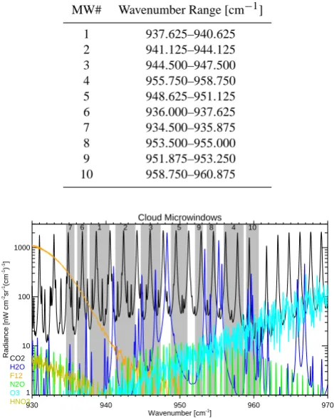
Microwindows (MWs) are small subsets of the MIPAS spec-trum of a few wavenumbers in width. A set of ten MWs have been selected from the MIPAS spectral range – and span the spectral region of 930–960 cm−1(Table 1). They are selected using a modification of the MIPAS MW selection algorithm (Dudhia et al., 2002) optimised for a joint retrieval of contin-uum radiance and temperature, in which the MWs are ranked in order of decreasing Shannon information content for non-scattering clouds. Figure 1 shows the positions of these mi-crowindows relative to molecular emission features. Note that each microwindow contains CO2lines (for the tempera-ture retrieval, discussed further in Sect. 2.3) whilst avoiding significant contributions from more variable gases such as H2O.
Table 1. Microwindows for cloud macrophysical parameter
re-trievals from MIPAS spectra, ordered in terms of priority of se-lection. Note that the boundaries are multiples of 0.125 cm−1so are consistent with both the “full-resolution” (0.025 cm−1grid) and “optimised-resolution” (0.0625 cm−1grid) spectra.
MW# Wavenumber Range [cm−1]
1 937.625–940.625 2 941.125–944.125 3 944.500–947.500 4 955.750–958.750 5 948.625–951.125 6 936.000–937.625 7 934.500–935.875 8 953.500–955.000 9 951.875–953.250 10 958.750–960.875
Cloud Microwindows
930 940 950 960 970
Wavenumber [cm-1
] 1
10 100 1000
Radiance [nW cm
-2sr -1(cm -1) -1]
1 2 3 5 4
6
7 9 8 10
CO2 H2O
F12
N2O
O3
HNO3
Fig. 1. Modelled full-resolution MIPAS spectrum for a tangent height of 9 km separated by constituent major emitters, in the spec-tral region of selected MWs listed in Table 1 – with MW specspec-tral regions shaded.
2.2 Continuum radiance
The Reference Forward Model (RFM) (Dudhia, 2005) is a standard radiative transfer model, which has been used here to pre-compute molecular transmittance spectra for each MW, τν, for each tangent height altitude, based on
clima-tological concentrations (Remedios, 2001). For each MW, it is then possible to identify nMW spectral points where molecular contributions are expected to be negligible (e.g. whereτν>0.95) using these pre-computed molecular
960.5 961.0 961.5 962.0 962.5 963.0
Wavenumber [cm
-1]
0
100
200
300
400
500
Radiance [nW/(cm
2
sr cm
-1)]
Fig. 2. Illustration of the continuum radiance, showing the RFM-simulated MIPAS radiance at 18 km (black), the corresponding transmittance spectrum (blue, multiplied by a factor of 400 for vis-ibility), the spectral points utilised to calculate the continuum radi-ance (red diamonds) along with the calculated continuum radiradi-ance (red solid line) for the spectral window considered, with the esti-mated uncertainty (red dashed lines).
The continuum radiance, R, and associated errorσ, can then be established by a simple mean and standard error for each radiance spectrum measured at each tangent height in a MIPAS scan pattern below about 25 km, such that
R= 1
nMW
X
i
L(νi, zF), (1)
whereL(νi, zF)is the measured radiance at theith masked wavenumber νi (in the particular MW) and FOV tangent
heightzF, and
σ= 1
nMW
s X
i
(L(νi, zF)−R)2, (2)
using standard deviation D such that the standard error is defined asD/√(n−1), wherenMWis the number of points averaged. By assigning an error value based on the actualD rather than the instrument noise, some allowance is made for any residual molecular contributions. Figure 2 illustrates the continuum radiance calculation process.
2.3 Cloud effective fraction
The next step is to identify the spectrum containing the cloud-top. One approach could be to use a simple thresh-old value on the continuum radiance, but since the
contin-uum radiance is a strong function of atmospheric tempera-ture and water vapour content as well as cloudiness, finding a suitable threshold value is difficult. The standard MIPAS Cloud Index (CI) method (Spang et al., 2004) attempts to overcome this temperature dependence by taking the ratio of radiance in two spectral regions (792–796 cm−1and 832– 834 cm−1) which react differently to cloud presence. Here, instead, it is preferable to have a scheme dependent upon the continuum radiance within each MW independently, as well as one having a more physical basis, since it parametrises the physical (geometrical and optical) fraction of the FOV filled with cloud. This is done via retrieval of a “Cloud Effective Fraction” (CEF) – a parameter first introduced by Hurley et al. (2009).
The CEF is defined as the fraction of the FOV covered by an optically thick, isothermal cloud with a horizontal cloud-top that would give the same continuum radiance as the ob-served cloud, assuming both have the same Cloud Top Tem-perature (CTT). Thus a single parameter α(the CEF), can be used to describe the infinite range possible of cloud ex-tinctions and spatial distributions within the actual FOV (al-though the concept of a single well-defined CTT in all such cases is questionable). Thusαvaries from 0 (cloud-free) to 1 (thick cloud completely filling the FOV) with intermediate values which may correspond either to thick cloud filling a small part of the FOV or thin cloud filling a larger fraction.
Mathematically,αfor a FOV having central tangent height zFis defined as
α=
Rzc−zF
−d (1−e
−kcs(z))φ (z)dz
Rd
−dφ (z)dz
, (3)
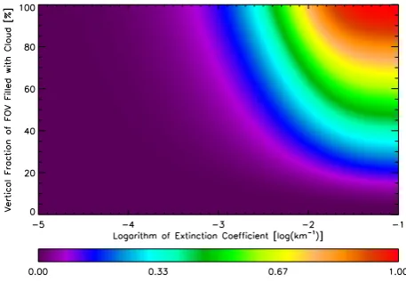
whereby the FOV can be described as extending a distance 2d in the vertical, zc is the cloud top height measured up-ward from the Earth’s surface,kcis the cloud extinction co-efficient along the limb path s, and φ (z)is the FOV verti-cal response function. Figure 3 shows the variation of α with extinction and the proportion of the FOV filled with cloud, as CEF is correlated with both. At low extinction (i.e.kc<10−4km−1), CEF is predominantly determined by extinction, however at the high extinction limit (ie. kc> 10−2km−1), CEF is highly correlated with the proportional filling of the FOV. In fact, a range of extinction and propor-tional FOV-fillings can combine to produce the same CEF, but outside the optically thin and thick limits, CEF is very much determined by both parameters – and is perhaps best thought of as an optical depth of sorts, normalised to the FOV in question.
From Eq. (3), it follows that, to good approximation,
α= R
Bc
, (4)
Fig. 3. Variation of CEF with extinction coefficient and the vertical proportion of the MIPAS FOV filled with cloud.
in Sect. 3.3.1) in the infrared, and thus increase the CEF. It is thus possible to obtain, from the Eq. (3) approximation, CEF>1, for scattering clouds. In practice, application to real MIPAS data does not show frequent examples of this, and operationally when this occurs, the CEF is then set to 1. Thisαis then used as the a priori value in the retrieval of the CEF, which is done prior to the full macrophysical retrieval. To retrieve the CEF from a single microwindow spectrum, it is assumed that the observed radiance can be represented as originating from a homogeneous path with the vertically lower fraction of the FOVαcorresponding to an optically thick cloud whilst the upper fraction of the FOV (1−α) originates from molecular emission features above the cloud but at the same local temperature as the cloud-top. Thus, the forward model for the measured spectrally varying radianceRνin order to better estimate the CEF via retrieval,
is approximated as
Rν=αBc+(1−α)Bc(1−τν), (5)
whereτν is the same pre-computed (climatological)
molec-ular transmittance used in Sect. 2.2. In practice, this works better ifBc is constrained by a priori information – for in-stance, by using a temperature climatology.
The CEF is retrieved using an iterative optimal estimation scheme (Rodgers, 2000):
xi+1=xi+
KTi S−y1Ki+S−a1
−1
(KTi S−y1(y−fi)−S−a1(xi−a)), (6)
where subscriptidenotes the iteration number, the state vec-torx contains the parameters to be retrieved, the measure-ment vectorycontains the measurements, f is the forward model (Sect. 2.5) applied to the current iteration ofx, K is the Jacobian matrix containing elements∂f/∂x, Syis the
er-ror covariance matrix ofy,ais the a priori estimate ofxand Sais the error covariance ofa.
In the case of the CEF retrieval, the state vector contains the CEF and a retrieved value of the Planck function, and the a priori vector contains the estimated CEFα, as calcu-lated from the continuum radiance, and the Planck function evaluated at the climatological for that tangent height. The measurement vector contains the spectrally varying radiance Lν, which the forward model Rν seeks to reproduce given
the appropriateαandBc.
Error on the measured spectrum is accounted for in the error covariance matrix
Sy=σn2In, (7)
for σn=NESR (the Noise Equivalent Spectral Radiance,
which for the case at hand is roughly 50 nW) and then×n identity matrix In. The uncertainty in the a priori is ac-counted for in the a priori covariance matrix Sa, such that Sa=
σ2
α 0
0 σB2 c
, (8)
taking the uncertainty in the estimated CEF to be σα2=
(1.0)2. The uncertainty in the blackbody radiance evaluated at the tangent height can be obtained from the expression
σB2
c=
∂B ∂T
¯
ν, TF
!2
σT2
F, (9)
whereσT2
F is the variance in the climatological temperature atzF, typically taken around 20 K to reflect the range of tem-peratures expected throughout the range of altitudes spanned by the FOV.
The retrieval error, stemming from the retrieval process it-self, given the uncertainties caused by noise on the measured spectra (in Sy), as well as uncertainties in the assumed a pri-ori (in Sa), is given by
Sx=
KTS−y K1 +S−a1 −1
. (10)
Once this retrieval for CEF has converged, the cloud-top is identified as lying in the highest altitude spectrum where the retrievedα >0.1. Finally, the retrieved value ofαis also used as a “measurement” in the macrophysical parameter re-trieval itself (Sect. 2.4). In principle, Eq. (5) also yields an “improved” estimate ofBc but, given the crudeness of this approximation, it is preferred to re-use the original climato-logical temperature profile.
2.4 Macrophysical parameter retrieval
2.4.1 State vector
The state vectorx contains the parameters to be retrieved, and in this case is defined as
x≡
zc
Bc
µc
, (11)
wherezc is the cloud-top height (CTH), Bc is the Planck function evaluated at the cloud-top temperatureTc(CTT) at the mid-point of the microwindow, and the logarithm of the extinction coefficient (CEX) is defined as
µc=log10kc, (12)
wherekc is the extinction coefficient (in km−1) measured along the limb line-of-sight. kc varies spectrally, and so theµcretrieved in each MW corresponds to the average ex-tinction in that MW – and any subsequent combination of MW results should keep this spectral variance in mind, even though it will be small in such a short spectral range.
In practice,kc is the extinction coefficient corresponding to the total extinction along the MIPAS limb path, including contributions from both atmospheric and cloud components of measured signal. However, as discussed in Sect. 2.1, the MWs in which the cloud properties are derived have been pre-selected such that the atmospheric contributions will be negligible in comparison with the cloud signal, having trans-mittance greater than 95%. Thus, to good approximation, the retrieved value ofkcwill correspond to the extinction of the cloud along the MIPAS limb path.
2.4.2 Measurement vector
The vectory, containing the measurements used for the re-trieval, is defined as
y≡
Ru
Rc
Rl
α
, (13)
whereRcis the continuum radiance (Sect. 2.2) from the FOV containing the cloud-top, having the retrieved cloud effec-tive fractionα, whileRuandRlare the continuum radiances from the FOVs immediately above and below, calculated in the same manner. The measurement covariance matrix Syis
diagonal, with variances given by the errors from the con-tinuum radiance and CEF retrieval. AlthoughRc andαare derived from the same spectrum, the argument is thatα de-pends on the spectral structure whereasRc is derived from the spectrally flat regions – and hence the two may be re-garded as independent.
The radianceRufrom the FOV above the cloud-top is ex-pected to have a value∼0 (since the CEF for this FOV will have been retrieved with a value<0.1, Sect. 2.3) and serves simply to constrain the retrieval from placing the cloud-top
too high. The inclusion of the CEF in the measurement vec-tor is discussed in the next section.
2.4.3 A priori information
This scheme essentially attempts to retrieve three macro-physical parameters from two non-zero continuum measure-ments,RcandRl. The usual method for dealing with such under-determined problems is to supply independent a pri-ori information. Due to the spatial inhomogeneity of cloud structures, obtaining useful direct a priori information on any of the three retrieved parameters is impractical – however, there are indirect a priori constraints on the relationships be-tween the retrieved parameters.
The first a priori constraint is represented by the CEF (α in Eq. 13) and is more conveniently introduced into the mea-surement vector (y) itself rather than in the conventional a priori vectora. This acts as a constraint on the CTH and CEX values, as described in Sect. 2.3.
A second source of a priori information is the background temperature profile obtained, for example, from climatology or meteorological analysis fields. Assuming this is not sig-nificantly perturbed in the presence of clouds, this acts as a constraint on the CTH and CTT, since the cloud-top tem-perature would be expected to correspond to a point on this profile.
Having identified the spectrum containing the cloud-top, the a priori estimate for the cloud-top height is set as the nominal tangent height for that measurementzF, and its cor-responding uncertaintyσzaset to±1 km. This corresponds to the range of the effective FOV width∼ ±1.5 km, since it is reasonable that this should envelope the uncertainty in cloud top height, if the cloud detection method is trustworthy.
For this altitude, the background temperature profile pro-vides an equivalent radianceBF, and uncertaintyσBFwhich is typically equivalent to a temperature uncertainty of±10 K. However, uncertainty with which zF represents the actual cloud-top height, and the variation of radiance with altitude
b=dB/dz(see Eq. 15) also have to be taken into account
when calculating the a priori covariance matrix elements. There is no reasonable a priori estimate for optical thick-ness so it is just set at a typical mid-range value (e.g. µa= −2.5) with a large uncertaintyσµa= ±0.5, to capture
the range of extinction for which the cloud forward model (Sect. 2.5) is applicable.
Thus the a priori vector is given by
a=
zF
BF
µa
. (14)
In addition, it is assumed that the Planck function (evalu-ated at the spectral mid-point of the microwindow in ques-tion) varies linearly with altitude within the cloud with a known gradient, such that
whereBc≡B(Tc)is the Planck function for the cloud top temperature, andb=dB/dzis the vertical gradient derived from an external (e.g. climatological) estimate of the back-ground atmospheric temperature profile. This vertical gra-dientb <0 in the troposphere andb >0 in the stratosphere, and is the radiance equivalent to the temperature lapse rate.
Assuming that the Planck function varies linearly with al-titude (Eq. 15) in order to estimate the uncertainty on the cloud top radiance, the a priori covariance matrix is given by
Sa=
σza2 b2σza2 0
b2σza2 σBF2 +b2σza2 0
0 0 σµ2
a
. (16)
2.5 Cloud forward model
The essential assumption within the macrophysical retrieval scheme is that a cloud can be represented as a homogeneous “grey” absorber characterised by the retrieved parameters. The cloud forward model (CFM)fcalculates the continuum radiance originating from a cloud described byzc,Tcandkc, and assumes that there is no spectral variation in absorption or in the Planck function over the limited spectral width of each microwindow.
2.5.1 Pencil-beams
The continuum radianceLt of an infinitesimal solid-angle pencil-beam viewing at tangent height zt within the cloud (i.e. zt< zc) is given by the standard radiative transfer equation for local thermodynamic equilibrium, assuming no molecular contributions from the atmosphere itself, and no scattering:
Lt=
Z
s
B(s)dτ
dsds, (17)
whereB(s)is the Planck function evaluated at the spectral mid-point of the microwindow along the paths, andτ (s)is the transmittance along the paths, given by
τ=exp(−kcs). (18)
Using simple circular geometry (ignoring refraction and as-suming the Earth’s radius,rez), the path distance and al-titude relative to the tangent point values are related by
(s−st)2'2re(z−zt). (19)
Eq. (17) can then be solved to give
Lt=
Bc+
b rekc2
(1−τ )−
bs
2rekc
(1+τ ). (20)
The appearance of the retrieved parameterkcin the denom-inator makes this potentially numerically unstable in the optically-thin limit, so a more computationally robust ap-proximation is preferred, such that
Lt'
Bc+
2
3b(zt−zc)τ
(1−τ ), (21)
which agrees with the exact solution in the asymptotic lim-its of transmittance. In the optically thick limit (τ =0) cloud effectively just emits from its upper surface andLt→ Bc, as expected. In the optically thin limit (τ →1), the emission effectively comes from the point one third of the vertical distance from the tangent point to the cloud-top, Lt→(13Bc+23Bt)(1−τ ), whereBt≡B(zt)from Eq. (15). 2.5.2 FOV convolution
The MIPAS FOV response function is represented by a ver-tical trapezium with a 4 km base and a 2.8 km top when projected onto the atmospheric limb. With tangent heights spaced at 3 km intervals for the original full-resolution surements, this gives a small overlap between adjacent mea-surements, but a much larger overlap for the 1.5 km spacing used in the “optimised-resolution” measurements employed since 2005.
This FOV function φ is sampled at N points (in prac-tice,N=9), which determine the altitudeszj for which the
pencil-beam calculations are performed. The measured con-tinuum radiance is then represented by a numerical convo-lution of the pencil-beam radiances at these altitudes (Ltj),
such that
R=
N
X
j=1
ajLtj, (22)
whereaj are coefficients of the normalised FOV
convolu-tion funcconvolu-tion at each pencil-beam altitudezj multiplied by
the “infinitestimal” integration step. Below the cloud-top, as the integration occurs at these finite points, the radiance is assumed to vary linearly between any two integration points – but at the cloud-top, there is a step function in radiance be-tween that emitted by the cloud, and that emitted by the clear atmosphere.
2.5.3 Cloud effective fraction
As mentioned in Sect. 2.4.2, the CEF defined in Eq. (4) is included in the measurement vector, therefore has to be eval-uated by the forward model. Using Eq. (22)
α=
PN
j=1ajLtj
Bc
. (23)
2.5.4 Definition of cloud forward model
Thus, the CFMf is simply Eq. (22) applied to each of the FOVs available in the measurement vectory, along with the definition of the CEF,α, given in Eq. (23). Furthermore, since these are analytic expressions, analytic derivatives are used to calculate elements of the Jacobian matrix K. 2.6 Combining microwindow results
2.6.1 Statistical combination
Retrievalsxk, and associated covariances Sxk, are obtained
from each of theM=10 microwindows. These results can then be combined using the standard statistical procedure for independent estimates, such that
ˆ
S−x1=
M
X
k=1
(Sxk)−1 and (24)
ˆ
x = ˆSx
M
X
k=1
(Sxk)−1xk, (25)
wherexˆ andSˆxrepresent the combined estimate and its
co-variance. There is an assumption here that the retrieved parameters do not vary spectrally – at least across the tens of wavenumbers represented by the selected microwindows (cloud-top radiances are converted to cloud-top temperatures prior to the combination). Extinction, of course, does vary spectrally – however over the small spectral range sampled by the MWs, this variation is also small. It also ignores the fact that the same a priori temperature climatology is used for each estimate, so the separate microwindow results are not strictly independent.
2.6.2 Spike tests
This combination step also allows a spike-test to be applied – that is, a removal of results from any microwindows which deviate significantly from the mean. Theχ2statistic is com-puted for each microwindow individually
χk2=(xk− ˆx)TSˆ−x1(xk− ˆx), (26)
and if the microwindow with the highestχ2 value exceeds the averageχ2by some factor (e.g. 2) its results are removed from the combination and the test repeated for the remaining microwindows.
2.6.3 Error inflation
In theory, the covarianceSˆxshould contain the random error
information on the retrieved values. However, it is recog-nised that this is an optimistic assumption since it makes no allowance for the forward model errors or approxima-tions, which have systematic components. If the different microwindows produce a large scatter of results, then the
standard deviation D of this distribution is likely to be a better estimate of the actual uncertainty, although this does not necessarily allow for forward model errors (see Sect. 3) either since all microwindows make the same assumptions. A three-element vector of scale-factors eis constructed to take the maximum of these to conservatively estimate the largest error likely to propagate through from the individual retrievals, such that
em=max
1,Dm
σm
, (27)
whereσmis the square root of the mth diagonal element in
the matrixSˆx(i.e. the uncertainty in parameterxmaccording
to the covariance matrix) andDmis the actual standard
de-viation of the parameterxmfrom the different microwindow
results.
The retrieval covariance is then “inflated” to produce the final covariance, such that
ˆ
S0x mm=e2mSˆx mm. (28)
2.7 Operational considerations
In an operational processor, it is desirable to have alterna-tive schemes available to perhaps retrieve fewer parameters in situations where the full retrieval fails due to an insuffi-cient number of microwindows providing retrievals which converge or pass the spike test, or if insufficient measure-ments are available, which happens most commonly when the cloud-top is detected in the lowest spectrum in the limb scan.
Assuming that a cloud-top has been detected somewhere in the scan, the operational algorithm attempts the following retrieval schemes in sequence until one returns valid results for at least three microwindows.
1. If available, using the measurement from the tangent height below the cloud-topRl(i.e. the cloud-top not lo-cated in the lowest tangent height in the scan), with a priori extinction information given byµa= −2.5 (i.e. mid-range value). This is the full three parameter re-trieval (zc,Tc,µc) from three measurements (Rc,Rl,α) plus the nominally zero radiance measurementRufrom the tangent height above the cloud-top, as described pre-viously.
2. As (1) but settingµa= −1.0, giving a “thick cloud” as-sumption (kc=0.1 km−1). Such a large initial guess value of extinction reduces the Jacobians with respect to this parameter to nearly zero, effectively leaving just two parameters (zc,Tc) to be retrieved from three mea-surements (Rc,Rl,α).
(zc,Tc) from only one tangent height using two mea-surements (Rc,α). This relies on the CEF retrieval in order to separate the two parameters.
3 Assessment of errors stemming from model assumptions
3.1 Retrieval error and real error
It must be noted that errors reported by the retrieval er-ror covariance matrix Sx describe only the erer-rors expected due to the statistical nature of an optimal estimations re-trieval process, and include only estimates of the uncertain-ties introduced into the retrieval by noise on the measure-ment, and by choise of the a priori estimates, as discussed in Rodgers (2000). Sx can be used to judge the convergence of a retrieval. However, it in no way encompasses the real error stemming from inaccuracies and insufficiencies in the forward model itself unless the forward model is physically complete. In this section, a thorough assessment of short-comings of the forward model – and the errors that are thus introduced – is carried out. As well, an assessment is car-ried out on how other pertinent atmospheric and instrument uncertainties can further add to the overall real error in re-trieved values.
Insufficiencies in the forward model are the dominant error sources, and errors propagating from such are often much larger than the retrieval error itself. As in any model, there are limits to the applicability of this algorithm. However, as long as the limits of applicability of this model, and the errors implicit because of the basic assumptions, are well known, it can be used within the discussed range of confidence. 3.2 Limitations of the cloud forward model: extinction
range of sensitivity
It is worth considering the optical thickness range over which the forward model is applicable. Consider first an optically thin cloud which completely fills the FOV. From the CFM, it follows that the total radiance in the FOV is
Rc=Bc
1−e−kcs'B
ckcs. (29)
The CEF of this thin cloud is
α=Rc
Bc
'kcs. (30)
Assuming a pathlength of approximately 300 km, and that clouds are detected only forα >0.1, this implies that the thinnest cloud which can be registered using this detection method has an extinction coefficient of 0.0003 km−1. Fur-thermore, for clouds having low optical depths (and in par-ticular, those having a vertically thin distribution of cloud particles), scattering becomes a non-negligible process, and the CFM is not sufficient to describe the emitted radiance.
However, such thin clouds are unlikely to be homogeneous in the MIPAS FOV, so even if scattering were included in the retrieval model, it is unlikely to give a significantly improved retrieval of the actual cloud properties. It should be noted, however, that the exclusion of scattering from the model thus introduces a systematic offset to the retrieved parame-ters as scattering generally acts to increase the radiance at these wavelengths.
Turning to the optically thick limit, assume that the extinc-tion is indistinguishable from infinity for path transmittances less than 1%:
τ=e−kcs=0.01. (31)
Given an estimated pathlength of 300 km, this yields that clouds withkc>0.015 km−1are indistinguishable from one another.
Therefore, it is reasonable to expect that extinction can be retrieved in the approximate range of−4≤µc≤ −2. 3.3 Limitations of cloud forward model: scattering
The process of scattering tends to increase the radiance emit-ted by a cloud. In the range of extinction coefficients between 10−4–10−2km−1, this is less than by a factor of two or three (see Sect. 3.3.1). This effect is accounted for in terms of for-ward modelling error in the retrieval process, but should be realised as a limitation of the model. The inclusion of scat-tering into this algorithm would imply that it could not be used operationally, as addition of scattering into any calcula-tion increases the computacalcula-tional cost of the problem dramat-ically. It also introduces extra uncertain cloud parameters to the problem, such as scattering particle characteristics, which is out of the scope of this work. In the “MIPclouds” project, microphysical cloud parameters are addressed in a separate microphysical cloud parameter retrieval (Spang et al., 2008). 3.3.1 Validation using KOPRA simulations
Whilst the forward model (CFM) discussed in the past few sections well describes an optically grey cloud, it is not nec-essarily a good representation of real clouds, which scatter radiation in and out of the line-of-sight. It is a useful exer-cise to compare the CFM with a more realistic model, which allows for scattering – and then to see how well the current retrieval is able to accurately retrieve the macroscopic param-eters of a more realistic cloud.
Fig. 4. Comparison of KOPRA (scattering and thus more realistic) and CFM (non-scattering) radiances, as a function of extinction co-efficient, as indicated by colour-scale (left panel). Relative radiance enhancement due to scattering is plotted on the right, with the range of extinction sensitivity in the CFM noted by dashed lines.
cirrus and liquid water clouds for a wide range of macro-and micro-physical cloud parameters, including atmospheric contributions as well as those resulting from the cloud pres-ence itself.
For the purposes of this exercise, mid-latitude cirrus cases from the database will be considered, as they form a typical and frequent class of high clouds detected by MIPAS. Mid-latitudinal cirrus has been modelled here as having cloud top heights between 6.5 km and 12.5 km, cloud depths between 0.5 km and 4 km, effective radii between 4.0 µm and 90.0 µm, volume densities between 1.1 m−3 and 1.1×10⁷m−3, and ice water content between 10.0−6g m−3and 1.0 g m−3, with microphysical parameters defined by Baran (2001). This results in clouds modelled with extinction coefficients be-tween approximately 10−5km−1 and 102km−1, although only cloud having CEX<−1 is considered here.
For the sake of argument, only KOPRA simulations with cloud top heights of 10.5 km and 11.5 km and cloud depths of 4.0 km are considered, even though for the 11.5 km case the lower FOV will not have the bottom 500 m cloud-filled as this represents a negligible radiance discrepancy. Figure 4 com-pares the radiances coming from KOPRA-simulated clouds and those calculated by the CFM presented here, for the con-sidered cases. The different cases are colour-coded by ex-tinction coefficient.
Given that the CFM seems able to represent single-scattering clouds (as modelled by KOPRA) to within an order of magnitude, it is interesting to see how well the macro-scopic retrieval can estimate the retrieved parameters, ap-plying the full three-parameter retrieval. Since KOPRA is a physically more rigorous model, this should give a met-ric of the skill with which the retrieval can determine cloud parameters for real clouds of various optical thicknesses.
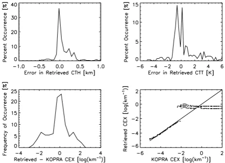
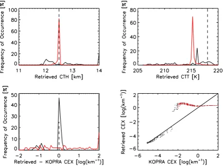
Fig. 5. Retrieved CTH, CTT and CEX for all KOPRA-simulated clouds having CTHs of 10.5–11.5 km, including those which are outside the purported range of applicability of the model. Top panels: probability distribution functions of difference between re-trieved and simulated CTH (left) and CTT (right) for KOPRA-simulated clouds. Lower left panel: probability distribution func-tion of the difference between KOPRA-simulated CEX and the re-trieved CEX. Lower right panel: scatterplot of rere-trieved CEX (right panel) for KOPRA-simulated clouds. Black line shows one-to-one division.
Again, considering the mid-latitudinal cirrus spectra used in the “MIPclouds” study, the macroscopic retrieval has been run to this end, the results of which are shown in Fig. 5.
It appears that the retrieval does a fairly consistent job of determining extinction, in the sense that it is able to differ-entiate between thin and thick cloud. For lower extinction values (<10−2km−1), the retrieval is able to make a rea-sonable estimate of the extinction, certainly retrieving CEX within 0.5 log(km−1). However, whilst the retrieval recog-nises cases of higher extinction as such, it does not usually get the extinction coefficient quite right for high cloud ex-tinction (see bottom right panel in Fig. 5), since the emitted radiance saturates toward the opaque limit, from values up-wards of 10−2–10−1km−1. It is these thick examples which cause the large error range in the lower left panel of Fig. 5.
In terms of the retrieved cloud top heights and cloud top temperatures, the retrieval tends to retrieve most cases to within 50 m and 1 K, although cases of higher error exist, up to≈500 m and≈5 K. Such instances of larger error generally correspond to cases of high cloud effective fraction (extinc-tions greater than about 0.1 km−1) when the retrieval tends to overestimate cloud top height and temperature, and to ac-cordingly underestimate the extinction.
asserted to be representative. These errors are not all random – rather the non-scattering CFM will systematically under-estimate the true radiance in the infrared which is measured due to scattering for a given set of macro- and micro-physical parameters by up to a factor of two or three, which will ef-fect the retrieved parameters. Thus, the CFM and retrieval based upon it work reliably within the design bounds and es-timated retrieval errors provided by the error covariance ma-trix Sx, well representing clouds for which scattering is not
the dominant radiative process, and for which the assump-tion of homogeneity is satisfied. As such, these error values do not represent the real range of errors expected when the algorithm is applied to real data, which is dominated by er-rors due to inhomogeneities in the cloud fields.
3.4 Limitations of cloud forward model: homogeneity
As a basic assumption of the CFM, the modelled cloud is assumed to fully-fill the horizontal domain of the FOV and to extend downwards to the surface of the Earth from the modelled cloud top height. Horizontal continuity across re-gions as big as the FOV is a realistic assumption for cirrus fields, which can extend in sheets for several hundreds of kilometres, although potentially not for individual clouds or lower cloud layers. Furthermore, obviously no cloud will ac-tually extend vertically in such a manner – this assumption is simply taken so that the cloud fills the modelled FOV to the bottom of the FOV below that in which the cloud top is identified. Since the FOV integration does not consider any pencil-beam radiance contributions beyond this, the effective cloud base is that of the lowest extent of that FOV. These as-sumptions have implications upon the retrieved parameters:
1. Optically-thin clouds contain good information on all three macrophysical cloud parameters discussed here – but particularly on CEX. However, in this case there is some sensitivity to the FOV-filling assumptions.
– Horizontal filling assumption: if, in reality, the cloud does not fully fill the horizontal (both across FOV, or along the FOV) extent of the FOV as as-sumed, the retrieved CEX will be less than the real cloud extinction value. Without further information (for example, imaging to show the horizontal extent of the cloud with respect to the measurement FOV), this remains an intractable problem.
– Vertical filling assumption: similarly, if the cloud does not extend vertically to the bottom of the low-est FOV considered in the CFM, a similar effect will be noticed. However, this effect should be min-imised because at these wavelengths most clouds should be opaque to radiation higher than the cloud base, for the extinction range of applicability.
2. Optically-thick clouds will have good information on cloud top height and temperature, but generally will not be sensitive to variations in extinction. Assump-tions on the relative filling of the FOV will thus affect the retrieved values of CTH and CTT, and the value of CEX will be fairly arbitrary, having a value reflecting a opaque or near-opaque cloud. Unless the cloud be-comes opaque below the cloud base is reached there will be a significant discrepancy in radiance measured in comparison to that expected by the CFM – and hence the CTHs should be underestimated.
Inhomogeneities are expected to be the sources of the dominant error in the retrieval, even though the magnitudes of such errors are not accounted for in any of the retrieval error estimates.
3.4.1 Using the CFM
Although not accurately representative for real scattering clouds, the clearest way to see the manner in which the re-trieval algorithm responds to clouds not satisfying the ho-mogeneity assumptions is to provide simulations using the CFM.
Case 1: horizontal inhomogeneity
A typical example of horizontal inhomogeneity is a cloud field filling the across-FOV horizontal extent of the FOV, which has an inconstant cloud top, or a inconstant extinction – or a combination of the two. A simple test of the behaviour of the retrieval algorithm is thus to model the FOV as fully-filled (up to the local CTHs) with two different clouds, each having a different CTH/CTT and CEX.
The FOV is considered to have two distinct clouds, which can be characterised by cloud top heights CTH1and CTH2, corresponding cloud top temperatures CTT1and CTT2, hav-ing extinctions CEX1and CEX2, which fill fractionsp1and p2of the FOV, respectively, such thatp1+p2=1. The CFM is used to simulate the radiance each cloud would emit if it were to homogeneously fill the full FOV up to its CTH (L1andL2, respectively), and then the two are combined to simulate the radiance emitted in the inhomogeneously-filled FOVLin, with each of them filling a particular fraction:
Lin=p1L1+p2L2. (32)
The effective cloud top height (CTHin), cloud top temper-ature (CTTin), and logarithm of cloud extinction along the limb path (CEXin) of the overall inhomogeneous FOV are defined as the fraction-weighted averages of the two sets of cloud parameters:
CTHin=p1CTH1+p2CTH2 (33)
CTTin=p1CTT1+p2CTT2 (34)
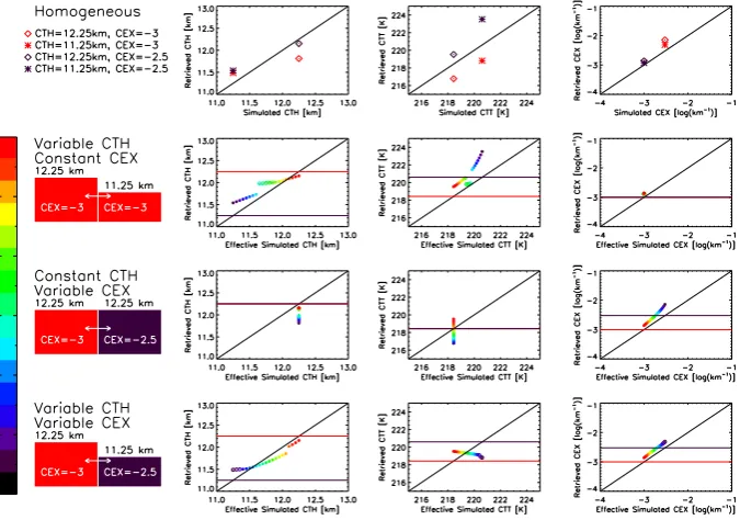
Clouds having CTHs of 11.25 km and 12.25 km, and CEXs of −2.5 and −3 are examined, as shown in Fig. 6, taking various perturbations of the FOV. The full three-parameter retrieval algorithm is then applied to the inhomo-geneous FOV radiances, the results of which are shown in Fig. 6.
In the first example, whereby the whole body of the cloud in the FOV has uniform extinction but varying CTHs, the CEX is very well retrieved. The effective CTH is retrieved to within 300 m, although the CTT is less consistently retrieved. When there are near equal proportions of both clouds in the FOV, the retrieval struggles to converge, as noted in the open symbols in Fig. 6.
Next, taking a constant CTH across the FOV, but varying the CEX between−3 and−2.5, generally the CEX is better retrieved for lower CEX than at the higher CEX end. The retrieved CEX is more-or-less proportional to the effective CEX in the FOV as the proportions of cloud shift – if not a little high in magnitude. Consequently, the CTH and CTT are retrieved representative of a lower cloud top than the ef-fective values, although the agreement is better when more of the FOV is filled with optically thin cloud.
Finally, both the CTH and CEX are allowed to vary, and the CTT is varied in accordance with the simulated CTH for each cloud. Retrieved CTHs and CEXs are highly correlated with the effective CTHs and CEXs of the FOV, whilst the CTT is rather poorly retrieved, as it balances the two cloud types by consistently retrieving the unweighted average of the two CTTs of the two clouds.
Case 2: vertical inhomogeneity
In order to test how the retrieval responds to cloud which is not vertically homogeneous in the instrumental FOV, the spe-cific case in which the vertical extent of the cloud is insuffi-cient to fill the appropriate FOVs fully down to their bottom-most extents are examined. This can be done by modifying the CFM for these purposes to simulate cloud having distinct cloud bottom heights (CBH), by changing the bounds of the path or FOV convolution integrations to simulate these inho-mogeneous cloudy states. To this end, cloud having CTH of 12.25 km and a CTT of 218.4 K are considered, having the 12 km FOV as the FOV in which the cloud top occurs. CBHs of 6.5–11.5 km are imposed, for clouds having extinction co-efficients between 10−3–10−1km−1. Thus, for the majority of CBHs, the lower FOV is not fully-filled vertically, and even the FOV in which the cloud-top is found is not filled for CBHs above 10 km (schematically shown in Fig. 7). The full three-parameter retrieval algorithm is then applied to CFM radiances, the results of which are shown in Fig. 7.
For clouds having extinction less than 10−2km−1, CTHs are still retrieved to within about 70 m, and the CTT is in-creased due partially to the anti-correlation between CTH and CTT, by less than a few degrees. Extinction values are decreased by roughly a half order of magnitude. Basically,
the retrieval recognises that there is less radiance than there should be for a given set of macrophysical parameters, and attempts to fit less cloud, in both an optical and geometric sense, throughout the FOV.
For thicker clouds, the CTH is usually significantly de-creased, and the retrieval attempts to balance CTT and CEX. Generally, CEX is overestimated – however there is little sen-sitivity to variations in CEX for such thick values of extinc-tion, and hence the retrieved values are rather arbitrary.
Finally, the retrieval fails to converge for CFM-modelled clouds thinner than 1 km, because this implies that the con-tribution to the bottom FOV is 0 by the cloud, and there is effectively one less measurement, since CBH is not parame-terised. This may, in reality, be a critical point, as many high clouds (such as cirrus) can be vertically very thin.
3.4.2 Using KOPRA simulations
KOPRA simulations can be used to quantify, with some sem-blance to real scattering clouds, the effect of inhomogene-ity on the retrieved parameters. Although it is impossible to quantify the errors coming from the infinite possible ar-rangements of inhomogeneous cloud in a MIPAS FOV, cases in which the CFM assumption of vertical homogeneity is vi-olated are considered to exemplify the magnitude of errors introduced from the assumption of homogeneity. These er-rors can be extended to horizontal inhomogeneity, whereby the same proportion of the FOV is taken to be cloud-free over the path sampled by MIPAS – although it should be noted that there will exist differences, depending upon the nature of the horizontal inhomogeneity.
Only a small proportion of the KOPRA simulations pre-pared for the “MIPclouds” study actually satisfy the assump-tions of homogeneity of the CFM. Cloud depths of 0.5 km through to 4 km are simulated – so there exist many cases in which the simulated cloud simply does not extend to the bottom of the considered 4 km MIPAS FOV. It is important to check how the retrieval model fares with respect to such cases, since it is likely that in real measurements there will frequently be cirrus which violate this assumption.
To this end, KOPRA simulations having a CTH of 12.5 km and cloud depths of 2.0 km, 3.0 km and 4.0 km are tested. These cloud depths represent fillings of the lowest FOV used in the measurement vector of between 6% and 65% of the FOV. Figure 8 shows the results of the retrieval algorithm applied to these simulations, where thin and thick clouds are said to be those having extinction coefficients along the limb path of less than and greater than 0.01 km−1, respectively.
Fig. 6. For varying cases of FOV filling and inhomogeneity (first row = homogeneous; second row = constant CEX, varying CTH; third row = constant CTH, varying CEX; final row = varying CEX and CTH), retrieved parameters of CTH (second column), CTT (third column) and CEX (last column) are plotted for varying proportions of filling by each cloud, from 100% the first cloud through to 100% the second cloud, with fraction varying linearly and indicated by colour. Filled circles mean retrieval has converged well – open circles mean it has been a retrieval with significant error.
5 K too low: the retrieval acts to attribute the lower radiance coming from the simulations to a lowered CTT.
In the case that the cloud is only 2 km deep, the model un-derestimates the the extinction by half an order of magnitude, and increases the CTH. Cases having depths of 3–4 km have the parameters retrieved closer to those simulated, although the model sometimes compensates for the missing radiance by lowering the CTT by up to about 10 K. The CFM/retrieval are probably “helped out” in a way because the effect of the extra radiation emitted by scattering clouds is partially can-celled out by the fact that there is simply not as much of the cloud as assumed. In any case, it appears that for inhomoge-neous clouds having small cloud depths the retrieval some-how manages to still retrieve more-or-less fairly reasonable values of CTH, CTT and CEX, even though this may be a re-sult of two CFM shortcomings partially cancelling each other out.
3.5 Water vapour continuum
At altitudes sampled by the lower tangent heights in the verti-cal MIPAS scan pattern (e.g. those less than about 6 km), the water vapour continuum is difficult to distinguish from the continuum radiance introduced by emitting clouds. Thus, re-gions of large water vapour concentration could become a potential issue for reliable cloud detection, which could lead to statistical offsets in retrieved cloud products. Although
this has not been studied in this work, in the current algorithm the absorption from the water vapour continuum is taken into account to some extent in the utilised molecular transmit-tance spectra, whereby the expected water vapour continuum is effectively “subtracted” from the measured continuum to establish the cloud contribution.
3.6 Pointing error
Pointing errors will make MIPAS tangent altitudes uncertain by several hundred metres – which is approximately the size of the largest uncertainties in the retrieved errors of CTH. The tangent altitudes are used only to help determine first-guesses for CTH and CTT, so as long as the a priori error ranges are set sufficiently large to encompass the range of pointing uncertainty (as they are in the current algorithm), errors in the pointing should not affect the final retrieved val-ues of CTH and CTT.
4 Application of algorithm
Fig. 7. Retrieved (first column) parameters of CTH (top row), CTT (second row) and CEX (third row), along with the difference between
the retrieved and simulated parameters (second column) for CFM-simulated clouds which do not satisfy the CFM assumptions of vertical homogeneity, as varied by clouds of different CBHs and CEXs. Bottom plot shows schematic of the relative position of each sampled CBH, with respect to the 9 km and 12 km FOVs.
values of CTH, CTT and CEX, even though this may be a re-sult of two CFM shortcomings partially cancelling each other out.
3.5 Water vapour continuum
At altitudes sampled by the lower tangent heights in the
ver-1240
tical MIPAS scan pattern (e.g. those less than about 6 km), the water vapour continuum is difficult to distinguish from the continuum radiance introduced by emitting clouds. Thus, Fig. 7. Retrieved (first column) parameters of CTH (top row), CTT (second row) and CEX (third row), along with the difference between the retrieved and simulated parameters (second column) for CFM-simulated clouds which do not satisfy the CFM assumptions of vertical homogeneity, as varied by clouds of different CBHs and CEXs. Bottom plot shows schematic of the relative position of each sampled CBH, with respect to the 9 km and 12 km FOVs.
Pathfinder Satellite Observation (CALIPSO) cloud climatol-ogy for cloud top height (Winker et al., 2009), and the Polar-ization and Anisotropy of Reflectances for Atmospheric Sci-ences coupled with Observations from a Lidar (PARASOL) cloud opacity records (Leroy et al., 1997; Deschamps et al., 1994).
4.1 Example results: 30 August 2009
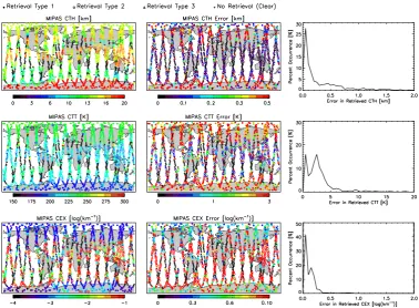
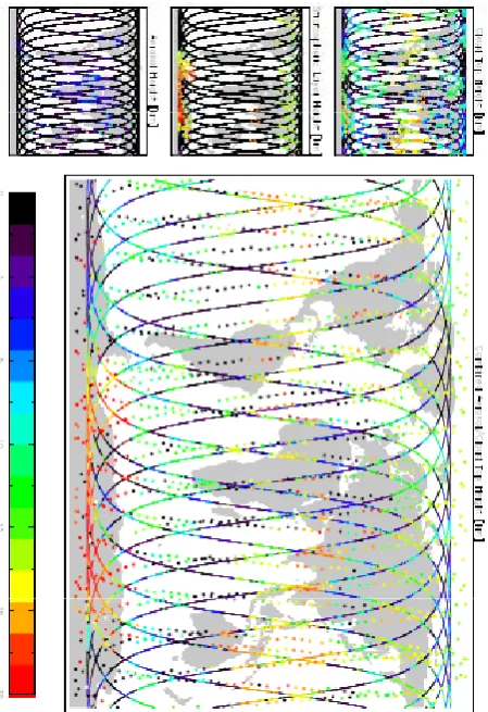
In this section, all measurements registered by MIPAS on 30 August 2009 have been processed using the described al-gorithm to highlight the products calculated and available
for further analysis. Figure 9 shows the retrieved values of CTH, CTT and CEX, along with the errors stemming from the retrieval process itself (from the retrieval error covariance matrix). Furthermore, the types of retrieval, as discussed in Sect. 2.7, are identified by different symbols – and profiles in which there is deemed to be no cloud present are identified by a cross, giving an indication of the proportion of verti-cal scans taken through the atmosphere having cloud present somewhere in the scan.