Remodelling of Lee’s Knife Diffraction Loss Model as a Function of Line of Site Percentage Clearance

(1)

http://www.sciencepublishinggroup.com/j/ijtam doi: 10.11648/j.ijtam.20170304.12

Remodelling of Lee’s Knife Diffraction Loss Model as a

Function of Line of Site Percentage Clearance

Swinton C. Nwokonko

1

, Vital K. Onwuzuruike

1

, Chibuzo Promise Nkwocha

2

1

Department of Electrical/Engineering, Imo State University, Owerri, Nigeria

2

Department of Chemical Engineering, Federal University of Technology, Owerri, Nigeria

Email address:

[email protected] (C. P. Nkwocha)

To cite this article:

Swinton C. Nwokonko, Vital K. Onwuzuruike, Chibuzo Promise Nkwocha. Remodelling of Lee’s Knife Diffraction Loss Model As a Function of Line of Site Percentage Clearance. International Journal of Theoretical and Applied Mathematics. Vol. 3, No. 4, 2017, pp. 138-142. doi: 10.11648/j.ijtam.20170304.12

Received: October 31, 2016; Accepted: January 6, 2017; Published: October 10, 2017

Abstract:

In this paper, remodeling of Lee’s piecewise knife diffraction loss model is presented. The original Lee’s piecewise knife diffraction loss model is expressed as a function of Fresnel-Kirchoff diffraction parameter. The computation of the Fresnel-Kirchoff diffraction parameter requires detailed terrain and link parameters. However, for quick link planning the Fresnel-Kirchoff diffraction parameter can be computed from the knowledge of the line of site percentage clearance alone. Moreover, in line of site link design, the required or acceptable obstruction clearance is specified in terms of line of site percentage clearance. Consequently, in this paper, the Lee’s model is remodeled into new piecewise functions that are entirely functions of line of site percentage clearance. The new version of Lee’s model is validated with the results of knife edge diffraction loss obtained from the original Lee’s piecewise knife diffraction loss model. With the new model it is easier to determine the diffraction loss that will be caused by any obstruction at a given line of site percentage clearance.

Keywords:

Diffraction Parameter, Diffraction Loss, Lee’s Diffraction Loss Model, Line of Site Communication, Percentage Clearance

1. Introduction

Diffraction is the bending of a wave around the edges of an opening or an obstacle [1]. Diffraction occurs when a wave encounters an object in its path or when the wave is forced through a small opening. The loss that occurs due to the obstacle in the path of the signal is known as “diffraction loss” [2]. The concept of diffraction is explained by the Huygens-Fresnel principle which states that each point on a wavefront acts as a point source [3-5]. This means that even if the direct path between the transmitter and receiver is blocked, some energy can reach the receiver from the portions of space that are visible to both the transmitter and receiver.

In order to estimate the losses caused by an obstacle in the signal path, it is usually assumed that the obstacle is a single knife-edge of negligible thickness or a thick smooth obstacle with a well-defined radius of curvature at the top [6], [7]. Where more than one obstacles are involved, then the obstacles are treated as multiple knife edge. In both cases, Fresnel zones are used by propagation theory to calculate

diffraction loss caused by obstruction located between the transmitter and receiver [8], [9]. The Fresnel zone in this case defines the cylindrical ellipsoidal path actually occupied by the signal as it propagates from the transmitter to the receiver. Fresnel zones are numbered starting from one and there is infinite number of Fresnel zones. The more the number of Fresnel zones obstructed, the higher the diffraction loss due to the obstruction. However, only the first 3 Fresnel zones have any real effect on radio propagation.

(2)

Furthermore, in most literatures studied, Lee’s piecewise function approximation of the graphical diffraction loss model is mostly used in knife edge diffraction loss computation. The Lee’s model is given a function of Fresnel-Kirchoff diffraction parameter. However, due to the simplicity of using the line of site percentage clearance, in this paper the piecewise functions in the Lee’s model are express in terms of LOS percentage clearance of Fresnel zone 1. The new version of Lee’s model is compared

with the diffraction loss computed from the original Lee’s model.

2. Theoretical Background

Lee developed piecewise model for estimating knife edge diffraction loss [9-11]. The Lee’s model defined the estimation of knife edge diffraction loss G(dB) in terms of Fresnel-Kirchoff diffraction parameter, V as follows:

G = 0 for < −1

G = 20log 0.5 − 0.62 for − 1 ≤ ≤ 0 G = 20log 0.5exp −0.95 for 0 ≤ ≤ 1

G = 20log 0.4 − "0.1184 − 0.38 − 0.1 %_{& for 1 ≤ ≤ 2.4} G = 20log '(.%%)_* + for > 2.4

-. /

(1)

The Fresnel-Kirchoff diffraction parameter ( at any given location between the transmitter and the receiver is given as [12-15];

= ℎ 12% 3 4&

ʎ 3 4 6 (2)

Where

ℎ is effective obstruction clearance height which is the height (in meters) from the tip of the obstruction to the line of site. λ is the wavelength of the radio wave in metres

Also, the radius of the nth Fresnel zone (r₇) is given as [16-20];

r8 = 289ʎ₃3 ₄4_&: (3)

where

; is the distance of location from the transmitter

< is the distance of location from the receiver

n is the nth Fresnel zone

λ is the wavelength of the radio wave in metres where;

ʎ =_>= (4)

where, c is the speed of a radio wave (c = 3x10@A/C); f is frequency of the radio wave in Hz.

Let D= 8 be the percentage LOS clearance for Fresnel zone n and let ℎ_{E= 8} be the clearance height corresponding to the percentage clearance D_{= 8}. Then,

ℎE= 8 = F_I((G H r₈& (5) In terms of D_{= 8} , the Fresnel-Kirchoff diffraction parameter V can be represented as ( _{E= 8} ) and it is given from Eq 2, Eq 3 and Eq 5 as;

E= 8 = ℎE= 8 12% _ʎ ₃3 ₄4&6 (6)

E= 8 = K √%8&F_I((G H M (7)

Accordingly, the Lee’s approximation for single knife edge diffraction loss, G as a function of _{E= 8} is given from Eq 1 and Eq 6 as;

G = 0 for E= 8 < −1

G = 20log 0.5 − 0.62 E= 8 for − 1 ≤ E= 8 ≤ 0 G = 20log 0.5exp −0.95 E= 8 & for 0 ≤ E= 8 ≤ 1

G = 20log K0.4 − 20.1184 − 0.38 − 0.1 E= 8 %M for 1 ≤ E= 8 ≤ 2.4

G = 20log K_*(.%%)_{NG H} M for E= 8 > 2.4 -. /

(8)

When the first Fresnel zone is considered, n =1, then

D= 8 = D= I;

E= I = K √%&F_I((G P M = '_R(.RI(STFG Q,P + (9) D= I = *Q,NG& I((

√% = 70.71068 E= I& (10)

If V = 1, then,

D= I = 70.71068 1 = 70.71068 % (11) If V = -1, then,

(3)

Table 1. _{The values of the diffraction parameter,} _{E= I}_{at the breakpoints and}

the corresponding values of LOS percentage clearance, W_{X Y}.

Z[X Y W_{X Y} %

-1 -70.71068

0 0

1 70.71068

2.4 169.7056

From Table 1, Eq 8 and Eq 9, Lee’s approximation for single knife edge diffraction loss, G as a function of LOS percentage clearance, D_{= I} is given as;

G = 0 for D= I < −70.7107% G = 20 log K0.5 − 0.62 ' FG P

R(.RI(ST+M for − 70.7107% ≤ D= I ≤ 0%

G = 20log K0.5exp −0.95 ' FG P

R(.RI(ST+M for 0 % ≤ D= I ≤ 70.7107%

G = 20log \0.4 − ]0.1184 − K0.38 − 0.1 ' FG P R(.RI(ST+M

%

^ for 70.7107% ≤ D= I ≤ 169.7056%

G = 20log _ (.%%)

K_ab.aPbcd`G P M e for D= I > 169.7056%

-. /

(13)

G = 0 for D= I < −70.7107% G = 20 log K0.5 − ' FG P

IIf.(fg)+M for − 70.7107% ≤ D= I ≤ 0% G = 20log K0.5exp − ' FG P

Rf.f@%%g%RS+M for 0 % ≤ D= I ≤ 70.7107%

G = 20log \0.4 − ]0.1184 − K0.38 − '_R(R.I(SRTI%FG P +M%^ for 70.7107% ≤ D= I ≤ 169.7056%

G = 20log K(.((@ITIgTI_F

G P M for D= I > 169.7056% -. /

(14)

3. Results and Discussion

Numerical computation of the diffraction loss with respect to diffraction parameter and percentage clearance in two different ranges are performed. Table 2 shows the results of the computation of diffraction loss for percentage clearance of 100% to -100%. In this paper, negative percentage clearance means that the tip of the obstruction is below the line of sight. Conversely, positive percentage clearance means that the tip of the obstruction is above the line of sight. Zero percentage clearance (0%) means that the tip of the obstruction is on the line of sight.

First, for every value of diffraction parameter, _{E= I} the corresponding percentage clearance, D_{= I} is computed

using D_{= I} = *NG P_√%& I((. In this case, the percentage clearance is with respect to Fresnel zone 1. Afterwards, the diffraction loss is computed using the diffraction parameter,

E= I and then the diffraction loss is computed using the

corresponding percentage clearance, D_{= I}. In Table 2, GdB ( _{E= I} ) is the diffraction loss computed from the diffraction parameter, _{E= I} whereas GdB (, D_{= I} ) is the diffraction loss computed from the percentage clearance, D= I. Table 2 shows that the two approaches give the same result (root mean square error is zero). Notably, at _{E= I} = 0, also, D= I = 0 and the diffraction loss obtained in both cases is GdB ( _{E= I} ) = GdB(D_{= I} ) = - 6.0206.

Table 2. _{Diffraction Loss Computed With Diffraction Parameter and With Respect To Percentage Clearance In The Range Of 100% To -100%.}

S/N Diffraction _Parameter,_Z h,[X

LOS Percentage Clearance, W_{X i}

GdB (Z_{[X Y} Diffraction Loss Computed from Z_h,[X

GdB (W_{X i}) Diffraction Loss Computed from W_{X i}

Error: GdB (Z_h,[X) – GdB (W_{X i})

Square Error

1 1.414214 100 -16.3604 -16.3604 0.0000 0

2 1.272792 90 -15.5728 -15.5728 0.0000 0

3 1.131371 80 -14.7614 -14.7614 0.0000 0

4 0.989949 70 -14.1893 -14.1893 0.0000 0

5 0.848528 60 -13.0223 -13.0223 0.0000 0

6 0.707107 50 -11.8554 -11.8554 0.0000 0

7 0.565685 40 -10.6884 -10.6884 0.0000 0

8 0.424264 30 -9.52146 -9.52145 0.0000 1E-10

9 0.282843 20 -8.3545 -8.35451 0.0000 1E-10

10 0.141421 10 -7.18755 -7.18755 0.0000 0

(4)

S/N Diffraction _Parameter,_Z h,[X

GdB (Z_{[X Y} Diffraction Loss Computed from Z_h,[X

GdB (W_{X i}) Diffraction Loss Computed from W_{X i}

Error: GdB (Z_h,[X) – GdB (W_{X i})

12 -0.14142 -10 -4.61716 -4.61718 0.0000 4E-10

13 -0.28284 -20 -3.40926 -3.40928 0.0000 4E-10

14 -0.42426 -30 -2.34901 -2.34904 0.0000 9E-10

15 -0.56569 -40 -1.40422 -1.40419 0.0000 9E-10

16 -0.70711 -50 -0.55218 -0.55216 0.0000 4E-10

17 -0.84853 -60 0.223687 0.223697 0.0000 1E-10

18 -0.98995 -70 0.9359 0.935903 0.0000 9E-12

19 -1.13137 -80 0 0 0.0000 0

20 -1.27279 -90 0 0 0.0000 0

21 -1.41421 -100 0 0 0.0000 0

RMSE 0.0000

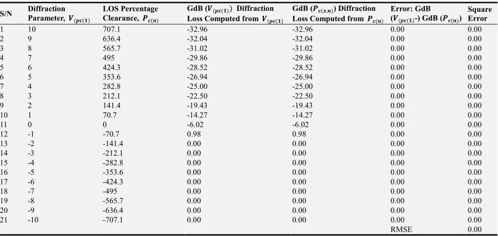
In the original Lee’s piecewise diffraction model, there are five functions that are used for different range of values of diffraction parameter, _{E= I}. Table 2 result does not have result for occasion when _{E= I} > 2.4. As such, Table 3 is used to show results for large values of _{E= I}. Again, Table 3 shows that the two approaches give the same result (root mean square error is zero).

Table 3. Diffraction Loss Computed With Diffraction Parameter and With Percentage Clearance In The range of 707% To -707%.

S/N Diffraction Parameter, Z_{[X Y}

GdB (Z_{[X Y} Diffraction Loss Computed from Z_{[X Y}

GdB (W_{X h,i}) Diffraction Loss Computed from W_{X i}

Error: GdB (Z_{[X Y}-) GdB (W_{X i})

1 10 707.1 -32.96 -32.96 0.00 0.00

2 9 636.4 -32.04 -32.04 0.00 0.00

3 8 565.7 -31.02 -31.02 0.00 0.00

4 7 495 -29.86 -29.86 0.00 0.00

5 6 424.3 -28.52 -28.52 0.00 0.00

6 5 353.6 -26.94 -26.94 0.00 0.00

7 4 282.8 -25.00 -25.00 0.00 0.00

8 3 212.1 -22.50 -22.50 0.00 0.00

9 2 141.4 -19.43 -19.43 0.00 0.00

10 1 70.7 -14.27 -14.27 0.00 0.00

11 0 0 -6.02 -6.02 0.00 0.00

12 -1 -70.7 0.98 0.98 0.00 0.00

13 -2 -141.4 0.00 0.00 0.00 0.00

14 -3 -212.1 0.00 0.00 0.00 0.00

15 -4 -282.8 0.00 0.00 0.00 0.00

16 -5 -353.6 0.00 0.00 0.00 0.00

17 -6 -424.3 0.00 0.00 0.00 0.00

18 -7 -495 0.00 0.00 0.00 0.00

19 -8 -565.7 0.00 0.00 0.00 0.00

20 -9 -636.4 0.00 0.00 0.00 0.00

21 -10 -707.1 0.00 0.00 0.00 0.00

RMSE 0.00

4. Conclusion

The remodeling of Lee’s piecewise knife diffraction loss model is presented. Original Lee’s piecewise knife diffraction loss model is expressed as a function of Fresnel-Kirchoff diffraction parameter. However, in this paper, the Lee’s model is expressed as a function of line of site percentage clearance. The new version of Lee’s model is validated with the results of knife edge diffraction loss obtained from the original Lee’s piecewise knife diffraction loss model and the new model presented in this paper.

References

[1] Allgood, D., Perkins, B., Asang, M., Simmons, C., Carroll, K., Tha, L., & Perez, T. (2014). Determination of the Optimal Aperture Size of a Pinhole Camera by Measuring Image Clarity.

[2] Kumar, S. (2015). Wireless Communications Fundamental & Advanced Concepts: Design Planning and Applications (Vol. 41). River Publishers.

[3] Tyson, R. K. (2015). Principles of adaptive optics. CRC press. [4] Tang, K., Qiu, C., Lu, J., Ke, M., & Liu, Z. (2015). Focusing and directional beaming effects of airborne sound through a planar lens with zigzag slits. Journal of Applied Physics, 117

(2), 024503.

[5] Stevanovic, N., & Markovic, V. M. (2016). Diffraction pattern by rotated conical tracks in solid state nuclear track detectors.

Optics & Laser Technology, 80, 204-208.

[6] Gálvez, M. A. (2010). Calculation of the coverage area of mobile broadband communications. Focus on land.

[7] Argota, J. A. R., Machado, M. M., Iglesias, I., & Ustamujic, S. (2012) Characterization tools for estimate radar signals with partial obstructions. ERAD 2012 - THE SEVENTH

EUROPEAN CONFERENCE ON RADAR IN

(5)

[8] Kapusuz, K. Y., & Kara, A. (2014). Determination of scattering center of multipath signals using geometric optics and Fresnel zone concepts. Engineering Science and Technology, an International Journal, 17(2), 50-57.

[9] Jude, O. O., Jimoh, A. J., & Eunice, A. B. (2016). Software for Fresnel-Kirchoff Single Knife-Edge Diffraction Loss Model.

Mathematical and Software Engineering, 2 (2), 76-84. [10] Rodriguez, I., Nguyen, H. C., Sørensen, T. B., Zhao, Z., Guan,

H., & Mogensen, P. (2016, October). A novel geometrical height gain model for line-of-sight urban micro cells below 6 GHz. In Wireless Communication Systems (ISWCS), 2016 International Symposium on (pp. 393-398). IEEE.

[11] Guo, W., Mias, C., Farsad, N., & Wu, J. L. (2015). Molecular versus electromagnetic wave propagation loss in macro-scale environments. IEEE Transactions on Molecular, Biological and Multi-Scale Communications, 1 (1), 18-25.

[12] Malila, B., Falowo, O., & Ventura, N. (2015, September). Millimeter wave small cell backhaul: An analysis of diffraction loss in NLOS links in urban canyons. In AFRICON, 2015 (pp. 1-5). IEEE.

[13] Héctor, J., Sturm, C., & Pontes, J. (2015). Radio Channel Fundamentals and Antennas. In Radio Systems Engineering

(pp. 81-106). Springer International Publishing.

[14] Lambrechts, J. W., & Sinha, S. (2015). Estimation of signal attenuation in the 60 GHZ band with an analog BiCMOS

passive filter. International Journal of Microwave and Wireless Technologies, 7 (06), 645-653.

[15] Bhuvaneshwari, A., Hemalatha, R., & Satyasavithri, T. (2015, January). Path loss prediction analysis by ray tracing approach for NLOS indoor propagation. In Signal Processing And Communication Engineering Systems (SPACES), 2015 International Conference on (pp. 486-491). IEEE.

[16] Ahamed, M. M., & Faruque, S. (2015, May). Path loss slope based cell selection and handover in heterogeneous networks. In 2015 IEEE International Conference on Electro/Information Technology (EIT) (pp. 499-504). IEEE.

[17] Sun, S., & Bancroft, J. C. (2002). Amplitude within the Fresnel zone for the zero-offset case. CREWES Research Report, 14. [18] Wang, H., Yang, K., Zheng, K., Yang, Y., & Ma, Y. (2016).

Estimation of electromagnetic field in air by a magnetic dipole in the sea based on a current sheet model. IET Microwaves, Antennas & Propagation, 10 (7), 709-718.

[19] Kopylov, Y. V., Popov, A. V., & Vinogradov, A. V. (1996). Diffraction phenomena inside thick Fresnel zone plates. Radio Science, 31 (6), 1815-1822.