Automatic Generation Control of Multi-area
Power System using Active Disturbance
Rejection Control
Y.V.L Charitha Reddy#1, Dr. M.S. Krishnarayalu#2#
Department of Electrical and Electronics Engineering V R Siddhartha Engineering College, Vijayawada, AP, India
Abstract - All national power system networks are multi-area networks interconnected by tie-lines. Automatic Generation Control (AGC) ensures the frequency and tie-line power errors are zero in the steady state so that nominal frequency and tie-line schedules are maintained. This can be achieved by sophisticated controllers. In this paper a three area power system is considered. The three areas consists of non reheat turbine thermal generator, reheat turbine thermal generator and hydro generator respectively. A control technique based on Active Disturbance Rejection Control (ADRC) is employed for this purpose. The resulting system is simulated using MATLAB Simulink software. The performance of ADRC is compared with classic PID Controller tuned by Zeigler-Nichols method. The outcome of ADRC is very good with low overshoots and minimum settling times.
Keywords: Multi-area Power System, Automatic Generation Control, Frequency error, Tie-line Power error, Active Disturbance Rejection Control, PID Control.
I. INTRODUCTION
Maintaining a nominal frequency and rated voltage within allowable limits is the most important requirement of power system operation. This ensures proper power system operation avoiding blackouts. Load Frequency Control (LFC) and Automatic Voltage Regulator (AVR) Control loops are mostly used in power systems to ensure quality power with rated frequency and voltage to the customer [1]-[2]. The scheme in which generation is adjusted automatically to restore the frequency to nominal value, as the system load changes continuously is called as Automatic Generation Control (AGC) which can make the interconnected power system more economic and reliable. The role of AGC is to divide the loads among system stations and generators so as to achieve maximum economy and to correctly control the scheduled interchanges of tie-line powers while maintaining a reasonable uniform frequency [3]-[5].
In order to improve the performance and stability of these control loops, proportional-integral-derivative (PID) controllers are normally used. But these fixed gain controllers fail to perform under varying load conditions and hence provide poor dynamic characteristics with a large settling time, overshoot and oscillations. In order to achieve a better dynamic performance, system stability and sustainable utilization of generating systems, PID gains must be well tuned [14]-[15]. Two main variables that change during transient power load are area frequency and tie line power interchanges. The concept of Load frequency control (LFC) is directly related to the aforementioned variables since the task is to minimize these variations. The key factor is to maintain the steady state deviations at zero. In this respect, effective measures like Active Disturbance Rejection Control (ADRC) have been developed that allow practical control [13].
ADRC as originally proposed by J. Han has three components namely tracking differentiator, nonlinear feedback control and nonlinear extended state observer. This triple combination proves to be a powerful tool for disturbance rejection control. It has been streamlined, simplified and parameterized so that it can be easily deployed across various hardware-software platforms and easily tuned by factory personnel in industry. In terms of design, the main parameters of focus in ADRC are the input and the output. This simply means that in order to perform its control tasks, the main information is analyzed from the input and output portions of the system. ADRC is able to detect the disturbance in the real system and also able to reject it. In this manner, its activity is very directed and efficient against the uncertainty in the system or any external disturbance [9]-[12].
II. LOAD FREQUENCY CONTROL
of LFC are to maintain reasonably uniform frequency, to divide the load between generators and to control the tie-line interchange schedules.
A. Mathematical Modelling of Load Frequency Control
1) Generator:
Generator is a device or machine which converts mechanical energy into electrical energy. Applying a small perturbation due to load change, the swing equation of a synchronous generator may be written as
2𝐺𝐻 𝜔𝑠
𝑑2∆𝛿
𝑑𝑡2 = ∆𝑃𝑚− ∆𝑃𝑒
In terms of small deviation in angular velocity
𝑑∆𝜔ω s 𝑑𝑡 =
1
2𝐻(∆𝑃𝑚− ∆𝑃𝑒) p.u, on base G Expressing angular velocity also in p.u on a base
𝜔s,
𝑑∆𝜔 𝑑𝑡 =
1
2𝐻(∆𝑃𝑚− ∆𝑃𝑒)
Taking Laplace Transform,
∆𝛺(𝑠) = 1
2𝐻𝑠(∆𝑃𝑚(𝑠) − ∆𝑃𝑒 𝑠 … (1)
Fig 1 Block Diagram of Generator
2) Load:
The load on a power system consists of variety of electrical loads. Resistive loads are frequency insensitive loads such as lighting and heating loads. Motor loads are frequency sensitive loads. Depending on the speed-load characteristics of the driven devices, the sensitivity of load with respect to frequency is known.
Hence the composite load change may be expressed as
∆𝑃𝑒 = ∆𝑃𝐿+ 𝐷∆𝜔 … (2)
∆𝑃𝐿= 𝑁𝑜𝑛 𝐹𝑟𝑒𝑞𝑢𝑒𝑛𝑐𝑦 𝑆𝑒𝑛𝑠𝑡𝑖𝑣𝑒 𝑙𝑜𝑎𝑑 𝑐𝑎𝑛𝑔𝑒
𝐷∆𝜔 = 𝐹𝑟𝑒𝑞𝑢𝑒𝑛𝑐𝑦 𝑆𝑒𝑛𝑠𝑡𝑖𝑣𝑒 𝑙𝑜𝑎𝑑 𝑐𝑎𝑛𝑔𝑒
𝐷 = 𝑃𝑒𝑟𝑐𝑒𝑛𝑡𝑎𝑔𝑒 𝑐𝑎𝑛𝑔𝑒 𝑖𝑛 𝑙𝑜𝑎𝑑 𝑃𝑒𝑟𝑐𝑒𝑛𝑡𝑎𝑔𝑒 𝑐𝑎𝑛𝑔𝑒 𝑖𝑛 𝑓𝑟𝑒𝑞𝑢𝑒𝑛𝑐𝑦
Fig 2 Block Diagram of Generator and Load
By elimination of the simple feedback loop, the above block diagram of the combined generator and load can be modified as
Fig 3 Block Diagram of Generator and Load
3) Turbine:
A turbine unit in power systems is used to transform the natural energy, such as the energy from steam or water, into mechanical power that is supplied to the generator. Generally there are three types of turbines available in power systems. They are Non-reheat, Reheat and Hydro turbines
Non-Reheat Turbine
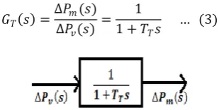
Non-reheat turbines are first-order units. A time delay occurs between switching the steam valve and producing the turbine torque. The transfer function can be of the non-reheat turbine is represented as
𝐺𝑇 𝑠 =
∆𝑃𝑚(𝑠) ∆𝑃𝑣(𝑠)
= 1
1 + 𝑇𝑇𝑠
… (3)
Fig 4 Block Diagram of Non-reheat Turbine
Reheat Turbine
𝐺𝑇 𝑠 =
∆𝑃𝑚(𝑠)
∆𝑃𝑣(𝑠)
=1 + 𝑠𝐾𝑇𝑇 1 + 𝑠𝑇𝑇
… (4)
Fig 5 Block Diagram of Reheat Turbine
Hydro Turbine
Hydraulic turbines are non-minimum phase units due to the water inertia. In the hydraulic turbine, the water pressure response is opposite to the gate position change at first and recovers after the transient response. Thus the transfer function of the hydraulic turbine can be represented as
𝐺𝑇 𝑠 =∆𝑃𝑚(𝑠) ∆𝑃𝑣(𝑠)
= 1 − 𝑠𝑇𝑤 1 + 0.5𝑇𝑤
… (5)
where 𝑇𝑤 is the water starting time.
For stability concern, a transient droop compensation part in the governor is needed for the hydraulic turbine. The transfer function of the transient droop compensation part can be represented as
𝐺𝑇𝐷𝐶 𝑠 =
1 + 𝑠𝑇𝐻1 1 + 𝑠𝑇𝐻2
… (6)
Fig 6 Block Diagram of Hydraulic Turbine
4) Governor:
The speed governor mechanism acts as a comparator whose output ∆𝑃𝑔is the difference between the reference set power ∆𝑃𝑟𝑒𝑓 and the power∆𝜔𝑅 (Load change).
∆𝑃𝑔 = ∆𝑃𝑟𝑒𝑓−1 𝑅∆𝜔
On applying Laplace transform,
∆𝑃𝑔 𝑠 = ∆𝑃𝑟𝑒𝑓 𝑠 − 1
𝑅∆Ω(s) … (7) The command ∆𝑃𝑔 is transformed through the hydraulic amplifier to the steam valve position command ∆𝑃𝑣. Considering a simple time constant
𝑇𝑔, the transfer function of the governor can be represented as
∆𝑃𝑣 𝑠 = 1
1 + 𝑇𝑔𝑠∆𝑃𝑔 𝑠 … (8)
Fig 7 Block Diagram of Governor
B. AGC of Single-Area Power System
By mathematical modeling of the governor, turbine, generator and load the scheme of the AGC for an isolated power system can be given as follows
Fig 8 AGC of isolated Power System
where B = frequency bias factor = 𝐷 +1
𝑅 𝐺𝐶 𝑠 = Controller transfer function ACE = Area Control Error
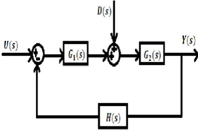
C. AGC of Multi-Area Power System
Consider two area represented by an equivalent generating unit interconnected by a lossless tie line with reactance 𝑋𝑡𝑖𝑒
Fig 9 Equivalent network of two area power system
𝑃12=𝐸1𝐸2
𝑋12 𝑠𝑖𝑛𝛿12 … (9)
where 𝑋12= 𝑋1+ 𝑋𝑡𝑖𝑒+ 𝑋2 and
𝛿12= 𝛿1− 𝛿2 … (10)
Assuming there is a small deviation in the tie-line flow from the nominal value
∆𝑃12= 𝑑𝑃12 𝑑𝛿12 𝛿
120
∆𝛿12= 𝑃𝑠∆𝛿12
The synchronizing power coefficient is defined as
𝑃𝑠= 𝑑𝑃12 𝑑𝛿12 𝛿
120
=𝐸1𝐸2
𝑋12 𝑐𝑜𝑠∆𝛿120
The tie-line power deviation then takes the form
∆𝑃12= 𝑃𝑠 ∆𝛿1− ∆𝛿2 … (11)
Conventional LFC is based upon tie-line bias control, where each area tends to reduce the Area Control Error (ACE) to zero. The control error for each area consists of a linear combination of frequency and tie-line errors
𝐴𝐶𝐸𝑖= ∆𝑃𝑖𝑗 + 𝐾𝑖∆𝜔𝑖 𝑛
𝑗 =1 ≠𝑖
… (12)
where Ki determines the amount of interaction during a disturbance in the neighbouring areas. For overall satisfactory performance Ki is equal to the frequency bias factor 𝐵𝑖.
𝐴𝐶𝐸𝑖 = ∆𝑃𝑖𝑗 + 𝐵𝑖∆𝜔𝑖
𝑛
𝑗 =1 ≠𝑖
… (13)
D. HVDC Link
A High Voltage Direct Current (HVDC) electric power transmission system uses direct current for the bulk transmission of electrical power, in contrast with the more common alternating current (AC) systems. For long-distance transmission, HVDC systems may be less expensive and suffer lower electrical losses. It allows power transmission between unsynchronized AC transmission systems. Since the power flow through an HVDC link can be controlled independently of the phase angle between source and load, it can stabilize a network against disturbances due to rapid changes in power.
It also requires fewer conductors per unit distance than an AC line, as there is no need to support three
phases and there is no skin effect.
Due to inherent technical and economic merits of DC transmission system over AC transmission systems, DC transmission systems have gained momentum for their development [3]. The DC link is simply represented by a transfer function as follows
𝐺𝐻𝑉𝐷𝐶 𝑠 =
𝐾𝑑𝑐 1 + 𝑠𝑇𝑑𝑐
… (14)
𝐾𝑑𝑐 = 𝐺𝑎𝑖𝑛 𝑜𝑓 𝐷𝐶 𝑙𝑖𝑛𝑘 𝑇𝑑𝑐 = 𝑇𝑖𝑚𝑒 𝐶𝑜𝑛𝑠𝑡𝑎𝑛𝑡 𝑜𝑓 𝐷𝐶 𝑙𝑖𝑛𝑘 III ACTIVE DISTURBANCE REJECTION
CONTROL
Active disturbance rejection control (ADRC) takes over from proportional–integral– derivative (PID) controller. ADRC generalizes the discrepancy between the mathematical model and the real system as a disturbance, and rejects the disturbance actively, hence the name active disturbance rejection control. It can simply be understood as a combination of an extended state observer (ESO) and a state feedback controller where ESO is utilized to observe the generalized disturbance, which is also taken as an extended state. The state feedback controller is used to regulate the tracking error between the real output and a reference signal for the physical plant [6]-[8].
The virtual state (sum of internal and external disturbances, denoted as total disturbance) is estimated online with a state observer and used in the control signal in order to decouple the system from the actual perturbation acting on the plant. Hence the states of nth order system along with disturbances are estimated by (n+1)th order Extended State Observer (ESO).
A. Design of ADRC for nth Order System
1) Plant Remodelling:
ADRC is developed for a general transfer function of a physical model considering it as a primary loop. General form of the physical model is represented with transfer function as
𝐺𝑝 𝑠 =𝑌(𝑠) 𝑈(𝑠)=
𝑏𝑚 +1𝑠𝑚+ 𝑏𝑚𝑠𝑚 −1+ ⋯ … … . +𝑏2𝑠 + 𝑏1 𝑎𝑛 +1𝑠𝑛+ 𝑎𝑛𝑠𝑛 −1+ ⋯ … … . +𝑎2𝑠 + 𝑎1 , 𝑛
≥ 𝑚 … (15)
where U(s) and Y(s) are input and output of the plant respectively. ai and bj are coefficients of transfer function.
By longhand division, the plant can be remodeled as
𝑠𝑛−𝑚𝑌 𝑠 = 𝑏
𝑜𝑢 𝑠 + 𝐷 𝑠 … (16) where
𝑏0= 𝑏𝑎𝑚 +1
𝑛 +1 … (17)
D(s) includes both internal and external disturbances. Hence after remodelling, the plant is of order n-m with high frequency gain of bo. The basic objective of ADRC is to implement a Extended State Observer (ESO) that can provide an estimate of disturbance d(t), such that it compensates the impact of d(t), on the process by means of disturbance rejection. Therefore the remaining is being handled by a simple proportional controller. Hence the disturbance is observed and cancelled by using ADRC.
2) Observer Gains:
Extended State Observer (ESO) is utilized to observe the generalized disturbance, which is taken as an extended state. Hence the state space mode of the system can be represented as
𝑆𝑋 𝑠 = 𝐴𝑋 𝑠 + 𝐵𝑈 𝑠 + 𝐸 𝑠 𝐷 𝑠 … (18)
𝑌 𝑠 = 𝐶𝑋 𝑠 … (19)
𝑋 𝑠 =
𝑥1 𝑠 𝑥2 𝑠
⋮ ⋮ ⋮
𝑥𝑛−𝑚 +1 𝑠 𝑛−𝑚 +1 ×1
𝐴 =
0
0
0
0
0
1
0
0
0
0
1
0
0
0
0
1
0
𝑛−𝑚 +1 × 𝑛−𝑚 +1
𝐵 = 0 0 ⋮ ⋮ ⋮ 𝑏𝑜
0 𝑛−𝑚 +1 ×1
𝐶 = [
1
0
0
]1×(𝑛−𝑚 +1)𝐸 = 0 0 ⋮ ⋮ ⋮
1 𝑛−𝑚 +1 ×1
The state space model of the disturbed process can be represented as
𝑠𝑍 𝑠 = 𝐴𝑍 𝑠 + 𝐵𝑈 𝑠 + 𝐿 𝑌 𝑠 − 𝑌 𝑠
where 𝑌 𝑠 = 𝐶𝑍 𝑠 ;
𝑍 𝑠 = 𝑍1 𝑠 𝑍2 𝑠 … . . 𝑍𝑛−𝑚 +1 𝑠 1× 𝑛−𝑚 +1 𝑇 ;
𝐿 = [𝑙1 𝑙2… . . 𝑙𝑛−𝑚 +1]1×(𝑛−𝑚 +1)𝑇
Assuming all the Eigenvalues of ESO are located at -𝜔𝑜, the observer gains are chosen as
𝑙𝑖 = 𝑛 − 𝑚 + 1𝑖 . 𝜔𝑜𝑖 , 𝑖
= 1,2, … , 𝑛 − 𝑚 + 1. … (20)
Hence by proper designing of ESO, 𝑍𝑖 𝑠 will be estimating the values of 𝑋𝑖 𝑠 closely. Then
𝑍𝑛−𝑚 +1= 𝐷 𝑠 ≈ 𝐷 𝑠
The generalized disturbance d(t) can be removed by the time domain estimated value 𝑥𝑛+1 with control law
𝑈 𝑠 =𝑈𝑜 𝑠 − 𝑍𝑛−𝑚 +1(𝑠) 𝑏𝑜
Now the system is reduced to a pure integral plant by substituting
𝑠𝑛−𝑚𝑌 𝑠 = 𝑏 𝑜.
𝑈𝑜 𝑠 − 𝑍𝑛−𝑚 +1 𝑠
𝑏𝑜 + 𝐷 𝑠
= 𝑈𝑜 𝑠 − 𝐷 𝑠 + 𝐷(𝑠) ≈ 𝑈0(𝑠)
3) Controller Gains:
The control law for the pure integral plant is
𝑈𝑜 𝑠 = 𝐾1 𝑅 𝑠 − 𝑍1 𝑠 − 𝐾2𝑍2 𝑠 − ⋯ ⋯
− 𝐾𝑛−𝑚𝑍𝑛−𝑚(𝑠)
To simplify the tuning process, all the closed-loop poles of the controller are set to -𝜔𝑐, 𝜔𝑐 represents the bandwidth of the controller. Then the controller gains have to be selected as
𝑘𝑖=
𝑛 − 𝑚
𝑛 − 𝑚 − 𝑖 + 1 𝜔𝑐𝑛−𝑚 −𝑖+1, 𝑖
= 1,2, … 𝑛 − 𝑚. … (21)
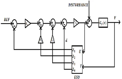
Increasing 𝜔𝑐 increases the tracking speed of the output of ADRC controlled system. The basic topology of the ADRC is given in Fig. 11.
Fig 11 Basic Block Diagram of ADRC
The above basic block diagram of ADRC is for a fourth order system. The proposed ADRC control is designed for non-reheat thermal, reheat thermal and hydraulic plants i.e. finding controller gains and observer gains using the plant transfer function for the respective plants. Here the reference inputs for ADRC are taken as Area Control Errors of the system i.e. ACE1, ACE2 and ACE3. The external disturbances for ADRC have been created by the load changes in the particular areas i.e. ∆𝑃𝐿1, ∆𝑃𝐿2
and ∆𝑃𝐿3. 𝐺𝑝(𝑠) represents the overall transfer function of the plant considered.
B. Design of ADRC for Non-Reheat Thermal Plant
Table I Data for Non-Reheat Thermal Plant
Governor Gain 𝐾𝑔1 1
Governor Time Constant 𝑇𝑔1 0.1 sec
Turbine Gain 𝐾𝑇1 1
Turbine Time Constant 𝑇𝑇1 0.4 sec Generator Inertia Constant 𝐻1 5 sec Frequency Sensitive factor 𝐷1 1.25 p.u
Change in Load ∆𝑃𝐿1 0.1 p.u Step Speed Regulation 𝑅1 0.05 p.u Synchronizing Coefficient 𝑃𝑠 22.6 p.u.
For the above data, the overall transfer function of primary loop of non-reheat thermal plant is
𝐺𝑝 𝑠 = 𝑌 𝑠 𝑈 𝑠
= 1
0.4𝑠3+ 5.05𝑠2+ 10.625𝑠 + 21.25 … (22)
From the plant transfer function n=3, m=0, a4=0.4, b1=1
Therefore from (17)
𝑏𝑜 = 1
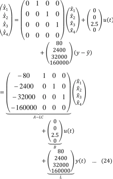
0.4= 2.5 … (23) The model of ESO is obtained as
𝑥 1
𝑥 2
𝑥 3
𝑥 4
=
0
0
0
0
1
0
0
0
0
1
0
0
0
0
1
0
𝐴
𝑥1 𝑥2
𝑥3 𝑥4
+ 0 0 2.5
0
𝐵
𝑢
+ 0 0 0 1
𝐸
𝑑
𝑦 =
1
0
0
0
𝐶𝑥1
𝑥2 𝑥3 𝑥4
𝑥 1
𝑥 2 𝑥 3
𝑥 4 =
0
0
0
0
1
0
0
0
0
1
0
0
0
0
1
0
𝑥 1
𝑥 2 𝑥 3 𝑥 4
+ 0 0 2.5 0 𝑢 𝑡 + 80 2400 32000 160000 𝑦 − 𝑦 =
0
0
0
160000
1
0
0
32000
0
1
0
2400
0
0
1
80
𝐴−𝐿𝐶𝑥 1 𝑥 2
𝑥 3 𝑥 4
+ 0 0 2.5 0 𝐵 𝑢 𝑡 + 80 2400 32000 160000 𝐿
𝑦 𝑡 … (24)
Controller gains, for 𝜔𝑐 = 10 𝑟𝑎𝑑/𝑠 , are obtained from (21) as
𝐾1= 1000 , 𝐾2= 300 , 𝐾3= 30
C. Design of ADRC for Reheat Thermal Plant
Table II Data for Reheat Thermal Plant
Governor Gain 𝐾𝑔2 1 Governor Time Constant 𝑇𝑔2 0.2 sec
Turbine Gain 𝐾2 0.5 Turbine Time Constant 𝑇𝑇2 0.4 sec
Generator Inertia Constant
𝐻2 5 sec
Frequency Sensitive factor
𝐷2 1.25 p.u
Change in Load ∆𝑃𝐿2 0.1 p.u Step Speed Regulation 𝑅2 0.05 p.u Synchronizing Coefficient 𝑃𝑠 22.6 p.u
The overall transfer function of primary loop of reheat thermal plant is obtained as
𝐺𝑝 𝑠 =
𝑌(𝑠) 𝑈(𝑠)=
1
4𝑠2+ 10.5𝑠 + 21.25 … (25) From the plant transfer function n=2, m = 0, a3 = 4, b1=1
From (17), (20) and (21)
𝑏𝑜 =1 4= 0.25
Observer Gains: 𝑙1= 60 ; 𝑙2= 1200 ; 𝑙3= 8000
Controller Gains: 𝐾1= 25 ; 𝐾2= 10
D. Design of ADRC for Hydro Plant
Table III Data for Hydro plant
Governor Gain 𝐾𝑔3 1 Governor Time Constant 𝑇𝑔3 0.2 sec
Water Time Constant 𝑇𝑊 1 sec Generator Inertia Constant 𝐻3 3 p.u sec
Transient Droop Compensation Time Constant
𝑇𝐻1 0.5 sec 𝑇𝐻2 0.513 sec Frequency Sensitive factor 𝐷3 1 p.u
Change in Load ∆𝑃𝐿3 0.1 p.u Step
Speed Regulation 𝑅3 0.05 p.u Synchronizing Coefficient 𝑃𝑠 22.6 p.u
Since Hydraulic plant consists of non-minimum phase turbine, an all pass filter is cascaded with the turbine in order to cancel out the positive zero and provide the necessary phase lead [9]. Hence the transfer function of the plant is given as,
𝐺𝑝 𝑠 =
𝑌(𝑠) 𝑈(𝑠) = 𝑠 + 1
0.6156𝑠3+ 4.3806𝑠2+ 26.713𝑠 + 21 … (26)
From the plant transfer function n=3, m=1, a4=0.6156, b2=1
From (17), (20) and (21)
𝑏𝑜= 1
0.6156= 1.624431
Observer Gains: 𝑙1= 60 ; 𝑙2= 1200 ; 𝑙3= 8000 Controller Gains: 𝐾1= 25 ; 𝐾2= 10
IV. TUNING OF PID CONTROLLER
A Proportional-Integrator-Derivative (PID) Controller is a control loop feedback mechanism which continuously calculates an error value as the difference between a desired set point and a measured process variable. The basic structure of PID controller is given by
𝐺𝑃𝐼𝐷 𝑠 = 𝐾𝑃+
𝐾𝐼
𝑠 + 𝐾𝐷𝑠 … (27)
where 𝐾𝑃, 𝐾𝐼 and 𝐾𝐷 are proportional, integral and
of the control loop has stable and consistent oscillations. Assuming the tuned proportional gain
to be 𝐾𝑢 with the oscillation period of 𝑇𝑢, the gain
constants of the PID controller are obtained as follows.
Case (i): Classic PID Controller
𝐾𝑃= 0.6𝐾𝑢 ; 𝐾𝐼=𝑇𝑢 ; 𝐾2 𝐷
=𝑇𝑢
8
… (28)
Case (ii): PID with some overshoot:
𝐾𝑃= 0.33𝐾𝑢 ; 𝐾𝐼=𝑇𝑢 ; 𝐾2 𝐷
=𝑇𝑢
3
… (29)
Case (iii): PID with no overshoot:
𝐾𝑃= 0.2𝐾𝑢 ; 𝐾𝐼=𝑇𝑢
2
; 𝐾𝐷
=𝑇𝑢
3
… (30)
For the system considered, 𝐾𝑢= 1.05 and 𝑇𝑢=
1.60.
Table IV PID gains by Zeigler Nichols Method
𝐾𝑃 𝐾𝐼 𝐾𝐷
Classic PID 0.63 0.8 0.2
PID (some overshoot) 0.3465 0.8 0.5333
PID (no overshoot) 0.21 0.8 0.5333
V. SIMULATION AND RESULTS
Simulation is carried out for the three area power system with ADRC and PID Controllers. A HVDC link is placed in parallel with HVAC tie line which is connected between area-1 and area-2. The basic structure of the three area system proposed is given below
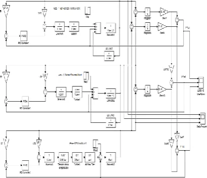
Fig 12 Proposed Three Area Power System
The three area AGC model using ADRC in Simulink is shown below
Fig 13 Simulation of Three Area Power System using ADRC
The three area AGC model using PID Controller in Simulink is shown below
Fig 15 Tie line power deviation of area-1
Fig 16 Tie line power deviation of area-2
Fig 17 Tie line power deviation of area-3
Fig 18 Frequency deviation of area-1
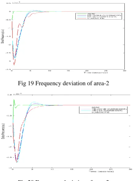
Fig 19 Frequency deviation of area-2
Fig 20 Frequency deviation of area-3
VI. DISCUSSION
ADRC and PID Controllers are employed as secondary controllers for the considered three area power system. The performances of these controllers are shown in Figs. 15-20. From these figures, it is observed that both the controllers brought the steady state frequency and tie line power deviations to zero. However PID controller tuned by Zeigler Nichols method for three different cases (Classic PID, No overshoot and Some overshoot) have large settling times and overshoots compared to the ADRC. The performance of ADRC, from Figs. 15-20, is clearly justified.
VII. CONCLUSIONS
Automatic Generation Control plays a key role in maintaining the changes in frequency and tie line powers to near zero. Thus it aims at reducing the steady state error, overshoots and settling times of the frequency and tie line power errors. ADRC, which is a robust control, acts as a secondary loop for AGC in improving its performance. Therefore the designed ADRC can reduce both the internal and external disturbances. The results of the three area power system, Figs. 15-20, clearly show that ADRC is much better compared to Zeigler-Nichols tuned PID Controller.
ACKNOWLEDGMENT
Vijayawada for providing the facilities to carry out this research.
REFERENCES
[1] Hadi Saadat, Power System Analysis, Tata McGraw-Hill Edition, New Delhi, 2002
[2] Arthur R.Bergen and Vijay Vittal, Power System Analysis, Second Edition, Pearson Education, 2006.
[3] Omveer Singh and Ibraheem Nasiruddin, “Optimal AGC regulator for multi-area interconnected power systems with parallel AC/DC links”, Cogent Engineering (2016), 3: 1209272
[4] Lili Dong and Yao Zhang, “On Design of a Robust Load Frequency Controller for Interconnected Power Systems”, 2010 American Control Conference Marriott Waterfront, Baltimore, MD, USA, June 30-July 02, 2010
[5] Zhiqiang Gao,Yao Zhang2, Lili Dong2, “Load Frequency Control for Multiple-Area Power Systems”, American Control Conference Hyatt Regency Riverfront, St. Louis, MO, USA, June 10-12, 2009.
[6] Saiteja and M.S. Krishnarayalu, “Load Frequency Control of Two-Area Smart Grid”, International Journal of Computer Applications (0975 – 8887) Volume 117 – No.14, May 2015.
[7] K. Nagarjuna and M.S. Krishnarayalu, “ADRC for Two Area-LFC”, International Journal of Engineering Research & Technology (IJERT) Vol. 3 Issue 11, November-2014.
[8] K. Nagarjuna and M.S. Krishnarayalu, “AVR with ADRC”, International Electrical Engineering Journal (IEEJ) Vol. 5 (2014) No.8, pp. 1513-1518.
[9] Z. Gao Shen and Gao Zhiqiang, “Active Disturbance Rejection Control for Non-minimum Phase Systems”
Control Conference (CCC), 2010 29th Chinese, 29-31 July 2010, pages 6066-6070
[10] Gang Tian and Zhiqiang Gao, “Frequency Response Analysis of Active Disturbance Rejection Based Control System”, 16th IEEE International Conference on Control Applications Part of IEEE Multi-conference on Systems and Control Singapore, 1-3 October 2007.
[11] Z. Gao, “Active disturbance rejection control: a paradigm shift in feedback control system design,” Proceedings of the American Control Conference, 2006:2399-2405.
[12] Gao, Z.; Huang, Y.; Han, J. “An Alternative Paradigm for Control System Design”, In Proceedings of the 40th IEEE Conference on Decision and Control, Orlando, Florida, USA, 4–7 December 2001.
[13] Jingqing Han, “From PID to Active Disturbance Rejection Control”, IEEE transactions on industrial electronics, vol. 56, no. 3, March 2009.
[14] Ashok Singh, Rmeshwar Singh, Rekha Kushwah, “Automatic Voltage Regulator and Automatic Load Frequency Control of Electrical Power Plant with Optimal Tuning Controller PID”, International Journal for Research in Applied Science & Engineering Technology (IJRASET), Volume 3 Issue X, October 2015, IC Value:13.98, ISSN:2321-9653.