http://www.sciencepublishinggroup.com/j/sjams doi: 10.11648/j.sjams.20190702.11
ISSN: 2376-9491 (Print); ISSN: 2376-9513 (Online)
Comparative Analysis of School Life Expectancy in Two
Randomly Selected Basic Schools in Ghana: Using Life
Table Functions and Survival Analysis
Bosson-Amedenu Senyefia
1, Danku Diaba Kafui
2, Opoku Frank
11Department of Mathematics and ICT, Holy Child College of Education, Takoradi, Ghana 2
Department of Languages, Holy Child College of Education, Takoradi, Ghana
Email address:
To cite this article:
Bosson Amedenu Senyefia, Danku Diaba Kafui, Opoku Frank. Comparative Analysis of School Life Expectancy in Two Randomly Selected Basic Schools in Ghana: Using Life Table Functions and Survival Analysis. Science Journal of Applied Mathematics and Statistics. Vol. 7, No. 2, 2019, pp. 8-14. doi: 10.11648/j.sjams.20190702.11
Received: March 26, 2019; Accepted: May 15, 2019; Published: June 4, 2019
Abstract:
This study applies life table functions and survival analysis to determine school life expectancy in Ghanaian private and public Basic Schools from grade 1 to grade 9 (JHS 3). The Kaplan Meier statistics such as Log Rank (Mantel-Cox), Breslow (Generalized Wilcoxon), and Tarone-Ware tests consistently showed a statistically significant difference between the male and female school dropout rate for private school pupils but showed statistically insignificant difference between male and female pupils’ dropout rate in public school pupils. The school life expectancy of grade 1 pupil in private and public schools were respectively found to be approximately 7 years for female and 8years for male; clearly showing that a grade one pupil in a private or public school who is a female has lower school life expectancy than the male counterparts. The survival curves for both private and public school cohorts showed that male pupils generally performed better than female counterparts. The survival curves and life table methods all established that peak dropout among male and female pupils generally occurred between grades 6 and 8 inclusive. It was also evident that average school life expectancy decreases with increasing age (i. e. with increasing grade levels). The study recommended further research to explore the effect of adolescent stage on the girl child education.Keywords:
Life Table Functions, Kaplan Meier, Demography, Survival Analysis, School Dropout, Life Expectancy1. Introduction
Life table techniques have been extensively employed in the measurement of mortality, survivorship and life expectancy of populations in many disciplines. They have been useful in many ways including measuring fertility, migration and population growth; application in making projections of population size; and for the assessment and adjustment of demographic deficient data. Life Tables are constructed based on a number of assumptions which includes that: migration is not allowed in the cohort, people die at each age according to a fixed schedule, radix is set at 1000, mortalities are evenly distributed at each age excluding the first 3 years of life. There are basically two groups of life tables, namely; Period or current Life Table and Cohort of Generational Life Table. The period Life Table which only
considers hypothetical cohorts deals with the mortality experience of diverse groups (cohorts) over a short period of time. For Generational Life Table on the other hand, deals with the mortality experience of a specific birth cohort. The data required here is annually based till all the members of the cohort die. Life tables are either complete or abridged. Complete (conventional) life table is fit for single aged data where mortality experience is considered annually throughout the life span. It is often carried out on large data for the calculation of rates, in the absence of which there will be systematic and random fluctuations. In the other side of the ledger, abridged life table are interval based i. e in terms of age group year intervals of 5 or 10 [1, 2-5].
with data collected from the university of Nigeria Teaching hospital. The study concluded that infant mortality was prevalent among the young population. Another study by Kovacheva (2017) sought to determine infant mortality by comparing life tables of Bulgaria and USA. As part of the findings of this study, the retirement age of Bulgarians which was 63 years was estimated to be reached by 74837 males and would live additional 15.6 years whereas females reaching 61 years will be 90061 in number and will live additional 20.6 years. On the other hand, USA with retirement age of 65 will have 80 724 males reaching it and will live additional 17.9 years. However, 88070 males were estimated to live additional 20.5 [1, 6-8].
Life table techniques have been applied to study the plant hopper on two rice species. The study was done under certain conditions including a temperature of than 27 degrees Celsius of temperature. The analysis of the raw data was based on the categories of age-stage and two-sex life. The main purpose for the two sex life table was for the life table to integrate the rate of variable development and the two sexes in the analysis. The study found that the species exhibited resistance to N. lugens. The study also found a decreased survival rate for preadult, low levels of longevity and fecundity. N. lugens was found to have potential of surviving and reproducing on both O. rufipogon and TN1 [9].
This paper seeks to measure the longevity length of life to be lived by boys and girls from grade one through to JHS 3 of their Basic School life. When these dynamics are known, will help institute interventions for any deficiency and facilitate the making of projections for proper planning purposes.
2. Method
A cohort of 73 pupils was studied from grade 1 through JHS 3 at a private school in Ghana. It was made up of 38 girls and 35 boys. Another cohort consisting of 78 pupils consisting of 38 male and 40 female were also studied from a Public School. Convenience sampling technique was adopted for the study due to data availability purposes.
Life table functions, their notations and relationships
makeup the anatomy of life table. A life table (LT) often have several categories including ndx, nqx, nLx, nlx, nPx, nMx. The first subscript ‘n’ denotes the number of completed years over which the interval extend. Again the subscript ‘x’ stands for exact age at which the interval begins. In the case of complete life table, the value of n is 1. Therefore the above life table functions reduces to dx, qx, Lx, lx, px, and Mx.
nm x: denotes the ratio of number deaths in the life table nd x to the population aged x at midyear.
nm x = . It is equivalent to ASDR in a stationary population at age x.
nL x: This represents the number of person – years that would be lived within the indicated age interval x and x + n by the cohorts of births assumed.
nL x = ( + nax . ndx) (1)
nax = , i. e assuming those who die during the interval lived the average n which is ½ the interval.
nL x = ( + 0.5. ndx)
Since nL x+n = + 0.5ndx) = ( − 0.5. ndx).
nL x = ( − 0.5 ( − ) )
nL x = n x−0.5n x − n x+n
∴ nL x = ( x + x + n) (2)
T
x: Denotes the total number of person years that would be lived after exact age x.
T x =
∑
=
w
x y
y
1
T0 = L0 + L1 + L2 + L3 + …. + L W (3)
: The average remaining lifetime in years for a person who survives at age x. It is tentatively known as the expectation of life.
e0 x is the expectation of life at birth = , [10-15].
3. Analysis
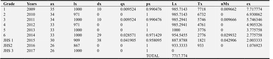
Table 1. School Life table of Private School male cohorts from 2009-2017.
Grade Years ax lx dx qx px Lx Tx nMx ex
1 2009 35 1000 10 0.009524 0.990476 985.7143 7718 0.009662 7.717774
2 2010 34 971 0 0 1 985.7143 6732 0 6.930062
3 2011 34 1000 10 0.009524 0.990476 985.2941 5746 0.009666 5.746346
4 2012 33 971 0 0 1 985.2941 4761 0 4.905326
5 2013 33 1000 0 0 1 1000 3776 0 3.775758
6 2014 33 1000 29 0.028571 0.971429 954.5455 2776 0.029932 2.775758
JHS 1 2015 30 909 38 0.041905 0.958095 887.8788 1821 0.042906 2.003333
JHS2 2016 26 867 0 0 1 933.3333 933 0 1.076923
JHS 3 2017 26 1000 0 0 1 0
TOTAL 7717.774
Table 1 applies the following methods; the column labeled Years represents the specific years considered in the study.
surviving pupils adjusted to a standard population size of 1000. The values are computed by finding the quotient of current ax and the original population size, and multiplying the result by 1000. The number of deaths (dx) denotes the change in population size from year x to year x+1 corrected to the nearest whole number. The sixth column denotes the mortality rate (qx) which is computed by dividing the current year’s dx by the current year’s lx. The seventh column (qx) represents the probability of living from age x to x+1. Since the individuals must either live or die in a particular year of life, qx+px = 1 and px = 1-qx. The eigth column (Lx) represents the years of life lived by the group between ages x and x+1. It is the average number alive during any particular year is computed by summing lx and lx+1 and multiplying the result by one-half. The ninth column (Tx) is the total number of person-years that would be lived after the beginning of the indicated age interval by cohorts of births (1000) assumed. It is calculated by cumulatively adding the Lx values from the bottom up. The total sum of Lx is the first
Tx corresponding to lx = 1000. The tenth column (Mx) represents the age specific death ratio at age x. It is computed by dividing corresponding dx by Lx. The eleventh column (ex) is the average remaining lifetime in years for a person who survives to the beginning of the indicated interval. It is computed by dividing Tx by its corresponding lx. Similar calculations were done in table 2.
Table 1 shows the school life table results for male pupils in a public school in Ghana. School life expectancy decreased with increased grade levels as well as increased age of pupils. The event (failure) did not occur in the second fourth, fifth, and 8 grades, recording zero probability of the event of failure for each grade. The probability of failure was high for grade 6 and 7 (JHS 1) with the peak at JHS 1. The school life expectancy of a grade one male pupil in private school was found to be approximately 8 years. The school life expectancies of male pupil in grade 2 through to JHS 2 are approximately 7years, 6 years, 5years 4years, 3yeras, 2 years and 1 year respectively.
Table 2. School life table results for female students in a private school in Ghana.
Grade Years ax lx dx qx px Lx Tx nMx ex
1 2009 38 1000 10 0.009524 0.990476 986.8421 7398 0.009651 7.398307
2 2010 37 974 19 0.019562 0.980438 959.8151 6411 0.019845 6.584747
3 2011 35 946 10 0.010068 0.989932 958.6873 5452 0.009934 5.763172
4 2012 34 971 0 0 1 985.7143 4493 0 4.625108
5 2013 34 1000 19 0.019048 0.980952 970.5882 3507 0.019625 3.507248
6 2014 32 941 19 0.020238 0.979762 939.3382 2537 0.020278 2.695201
JHS 1 2015 30 938 86 0.091429 0.908571 818.75 1597 0.104689 1.70381
JHS2 2016 21 700 29 0.040816 0.959184 778.5714 779 0.036697 1.112245
JHS 3 2017 18 857 0 0 1 0
TOTAL 7398.307
Table 2 shows the school life table results for female students in a private school in Ghana. School life expectancy decreased with increasing grade levels as well as with increasing age of pupils. The event (failure) did not occur in the fourth grade, recording zero probability of the event of failure for the fourth grade. The probability of failure was high for JHS1 and grade 8 (JHS2) with the peak at grade 7 (JHS 1). The school life expectancy of a grade one female pupil in public school was found to be approximately 7 years. The school life expectancies of female pupil in grade 2 through to JHS 2 are approximately 7years, 6 years, 5years 4years, 3yeras, 2 years and 1 year respectively.
3.1. Comparison of Results of Tables 1 and 2
The probability of female pupils dropping out of school in JHS1 in private school was higher for female pupils (qx = 0.091429) compared to male pupils (qx = 0.041905). However, the probabilities of a private school female pupil dropping out of school was higher for JHS 1 and JHS 2 than male pupils from private school. Again, the school life expectancy of female and male pupils of grade 1 in private school was respectively found to be approximately 7years and 8years; clearly showing that a grade one pupil in a private school who is a female has lower school life expectancy than the male counterpart.
Figure 1. Graph displaying mortality rates in Private school Boys and Girls from grade1 to JHS 3.
Figure 2. Life expectancy of boys and girls in the Basic School.
Figure 2 makes it evident that average life expectancy of boys is generally greater than girls from lower to higher age levels. However, there seems to be approximately equal average life expectancy rates at grade 3 and grade 4 between
boys and girls. It is also evident that average life expectancy (basic school dropout rate) decreases with increasing age (i. e. with increasing grade levels).
Table 3. Case Processing Summary for private Basic school cohorts.
Treatment Total N N of Events Censored
N Percent
female 38 20 18 47.4%
male 35 9 26 74.3%
Overall 73 29 44 60.3%
The table shows the Case Processing Summary. The number of event for female was 20 out of 38 and the number of event for male was 9 out of 35 To this end, in terms of number of events, the two treatments did not perform in a similar fashion. The percentage censored was high for each group (i. e. 47.4% and 74.3% for female and male respectively).
Table 4. Means and Medians for Survival Time for private school.
Treatment
Meana
Estimate Std. Error 95% Confidence Interval
Lower Bound Upper Bound
female 7.711 .311 7.101 8.320
male 8.257 .338 7.594 8.920
Overall 7.973 .229 7.524 8.422
The mean value of male (8.257) was higher than that of the female (7.711). There is quite some difference between the two treatments and there is the need to find out if the difference is statistically significant.
Table 5. Overall Comparisons for private Basic school cohorts.
Chi-Square df Sig.
Log Rank (Mantel-Cox) 4.925 1 .026
Breslow (Generalized Wilcoxon) 4.922 1 .027
Tarone-Ware 4.961 1 .026
The Log Rank (Mantel-Cox) method tests the equality of
survival functions with all the points in time weighted equally. Breslow (Generalized Wilcoxon) test the equality survival functions by weighing the time points based on the number of cases at risk in each time point. Tarone-Ware tests the equality survival functions by weighting the points of time by the square root of the number of cases. All the three methods were used to check the consistency of the results. By all three statistics used, there was a statistically significant difference between the male and female school dropout rate (i. e 0.026 < 0.05, 0.027 < 0.05).
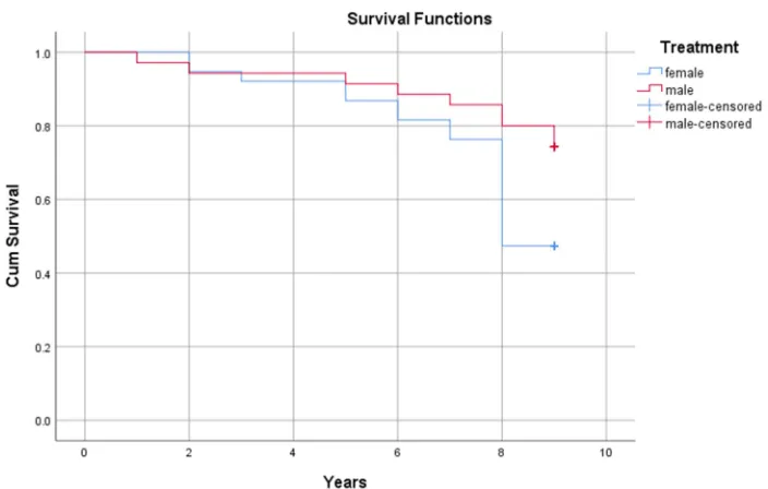
The curve in red is the survival curve for male and the blue survival curve is for the female. The small vertical blue and red lines represent female-censored and male censored respectively. It can be seen that the censored outcomes are all at 9 years. Every part of the curves that shows a vertical drop or line is an indication of a dropout or the event. By studying
the two survival function plots, it is evident that the male pupils performed better at each of the time points. This is because the probability of males is higher at every point in time except between the first and second year. By further analysis of the curve shows a peak dropout among female pupils at the eighth year (JHS2).
Table 6. School Life Table for Public School Female Cohort from 2009-2017.
Grade Years ax lx dx qx px Lx Tx nMx ex
1 2009 40 1000 21 0.020619 0.979381 975 7478.167 0.021147 7.478167
2 2010 38 950 0 0 1 975 6503.167 0 6.845439
3 2011 38 1000 31 0.030928 0.969072 960.5263 5528.167 0.032199 5.528167
4 2012 35 921 10 0.011193 0.988807 946.2406 4567.641 0.010895 4.959153
5 2013 34 971 0 0 1 985.7143 3621.401 0 3.727912
6 2014 34 1000 41 0.041237 0.958763 941.1765 2635.686 0.043814 2.635686
JHS 1 2015 30 882 52 0.058419 0.941581 857.8431 1694.51 0.060088 1.920444
JHS2 2016 25 833 41 0.049485 0.950515 836.6667 836.6667 0.049287 1.004
JHS 3 2017 21 840 0 0 1 0
TOTAL 7478.167
Table 6 shows the school life table results for female students in a public school in Ghana. School life expectancy decreased with increased grade levels as well as increased age of students. The event (failure) did not occur in the second and fifth grades, recording zero probability of the event of failure for each grade. The probability of failure was
high for grade 6 through to grade 8 (JHS2) with the peak at grade 8 (JHS 2). The school life expectancy of a grade one female pupil in public school was found to be approximately 7 years. The school life expectancies of female pupil in grade 2 through to JHS 2 are approximately 7years, 6 years, 5years 4years, 3yeras, 2 years and 1 year respectively.
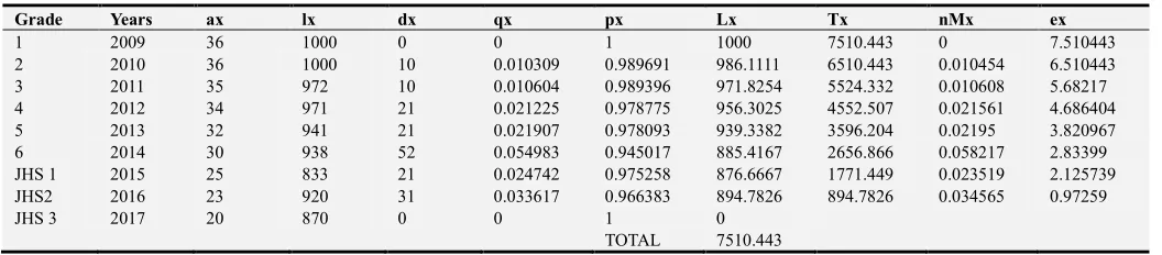
Table 7. School Life Table for Public School Male Cohort from 2009-2017.
Grade Years ax lx dx qx px Lx Tx nMx ex
1 2009 36 1000 0 0 1 1000 7510.443 0 7.510443
2 2010 36 1000 10 0.010309 0.989691 986.1111 6510.443 0.010454 6.510443
3 2011 35 972 10 0.010604 0.989396 971.8254 5524.332 0.010608 5.68217
4 2012 34 971 21 0.021225 0.978775 956.3025 4552.507 0.021561 4.686404
5 2013 32 941 21 0.021907 0.978093 939.3382 3596.204 0.02195 3.820967
6 2014 30 938 52 0.054983 0.945017 885.4167 2656.866 0.058217 2.83399
JHS 1 2015 25 833 21 0.024742 0.975258 876.6667 1771.449 0.023519 2.125739
JHS2 2016 23 920 31 0.033617 0.966383 894.7826 894.7826 0.034565 0.97259
JHS 3 2017 20 870 0 0 1 0
TOTAL 7510.443
Table 7 shows the school life table results for male students in a public school in Ghana. School life expectancy decreased with increased grade levels as well as increased age of students. The event (failure) did not occur in grade 1 but occurred throughout other levels. The probability of failure was more intense for grade 6 through to grade 8 (JHS2) with the peak at grade 8 (JHS 2). The school life expectancy of a grade one male pupil in public school was found to be 8 years. The school life expectancies of male pupil in grade 2 through to JHS 2 are 7 years, 6 years, 5 years, 4 years 3 years, 2 years, and 1 year respectively.
3.2. Comparison of Results of Tables 6 and 7
The probability of male pupils dropping out of school in Grade six in public school was higher for male pupils (qx = 0.054983) compared to female pupils (qx = 0.041237). However, the probabilities of a public school female pupil dropping out of school was higher for JHS 1 and JHS 2 than
male counterparts. Again, the school life expectancy of female and male pupils of grade 1 in public school was respectively found to be approximately 7 years and 8 years; clearly showing that a grade one pupil in a public school who is a female has lower school life expectancy than the male counterpart.
Table 8. Means and Medians for Survival Time for public Basic school cohorts.
Treatment Meana
Estimate Std. Error
95% Confidence Interval Lower Bound Upper Bound
male 7.972 .280 7.424 8.520
female 7.821 .329 7.176 8.465
Overall 7.893 .214 7.473 8.314
Table 9. Overall Comparisons for public Basic school cohorts.
Chi-Square df Sig.
Log Rank (Mantel-Cox) .209 1 .648
Breslow (Generalized Wilcoxon) .208 1 .648
Tarone-Ware .206 1 .650
All four statistics showed that there is no statistical significant difference between male and female dropout rates in the public school (i. e P > 0.05).
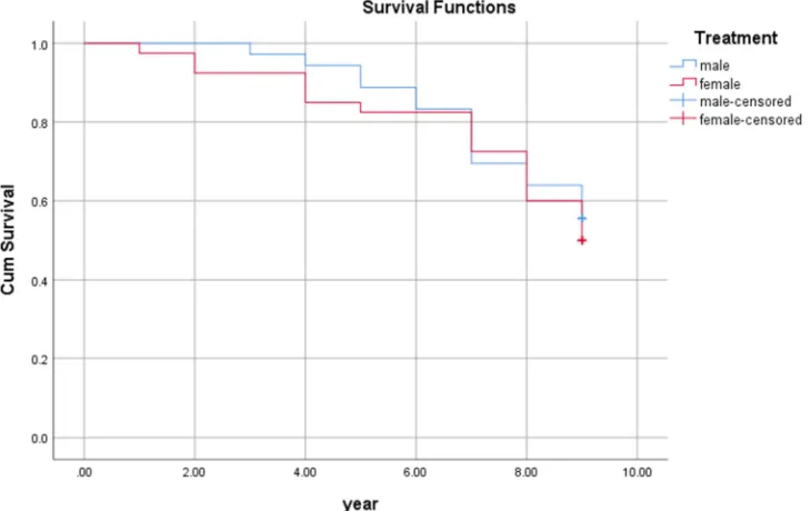
The figure shows that in general male pupils performed better right from the 1st to the 7th year, as the number that experienced the event was fewer compared to the female pupils. However, between 7th and 8th year there was greater mortalities (dropout). From the eight to the ninth year, there was more mortality in female pupils than males. Both male and female categories have a number of pupils who were censored at the end of the 9th year as they did not experience the event of interest.
Figure 4. Survival Plot for male and female public school pupils’ enrolment.
4. Conclusions
The study measures the longevity length of life to be lived by boys and girls from grade one through to JHS 3. The Kaplan Meier statistics including Log Rank (Mantel-Cox), Breslow (Generalized Wilcoxon), and Tarone-Ware tests consistently showed a statistically significant difference between the male and female school dropout rate for private school pupils but showed statistically insignificant difference between male and female pupils dropout in public school. The school life expectancy of female and male pupils of grade 1 in private and public schools were respectively found to be approximately 7years and 8years; clearly showing that a grade one pupil in a private or public school who is a female has lower school life expectancy than the male counterparts. The survival curves for both private and public school cohorts showed that male pupils generally performed better than female counterparts. The survival curves and life table methods all established that peak dropout among male and female pupils generally occurred between grades 6 and 8 inclusive. It was also evident that average school life expectancy decreases with increasing age (i. e. with increasing grade levels). The study recommended further research to explore the effect of adolescent stage on the girl child education.
5. Recommendations
As part of the recommendations of this paper,
1.Future studies should delve into factors that account for high level of dropout rates among basic school pupils particularly among females in JHS.
2.JHS pupils should be encouraged and sensitized on the need for them to visit counseling units at their schools. 3. Further studies should look into the effect of adolescent
stage on JHS pupils.
Implication for Future Research
Future research can explore the effect of adolescent stage on the girl child education. This is because high mortalities (drop outs) were realized between grade 6 and 9, a period of beginning of adolescent stage.
Future Research
References
[1] Kovacheva T. P (2017). International Mathematical Forum, Vol. 12, 2017, no. 10, 469 - 479. HIKARI Ltd, www.m-hikari.com. https://doi.org/10.12988/imf.2017.7225.
[2] Pollard, J. H. (1998). Keeping abreast of mortality change. Actuarial and Demography Research Paper Series, No. 002/98. [3] Renshaw, A. E. & Haberman, S. (2000). Modelling for
mortality reduction factors (Actuarial Research Paper No. 127). Department of Actuarial Science and Statistics, City University, London.
[4] Renshaw, A. E. & Haberman, S. (2006). A cohort-based extension of the Lee^Carter model for mortality reduction factors. Insurance: Mathematics and Economics, 38, 556-570.
[5] Tabeau, E., Van Den Berg Jeths, A. & Heathcote, C. (eds.) (2001a). Forecasting mortality in developed countries: insights from a statistical, demographic and epidemiological perspective. Kluwer Academic Publishers, Dordrecht. [6] Igwenagu C. M. (2014). The Application of Life Table
Functions: A Demographic Study. e-ISSN: 2278-5728, p ISSN: 2319-765X Volume 10, Issue 1 Ver. IV. (Feb. 2014), PP 80-82 www.iosrjournals.org.
[7] United Nations (1983), Manual X: Indirect Techniques for Demographic Estimation, New York: United Nations,
available online at:
http://www.un.org/en/development/desa/population/publicatio ns/manual/estimate/demographic estimation.shtml.
[8] Beaujouan, Éva and Tomáš Sobotka, Late Motherhood in Low-Fertility Countries: Reproductive Intentions, Trends and Consequences, VID Working Paper 2/2017 and Human Fertility Database Research Report HFD RR-2017.
[9] Liang-Xiong Hu, Hsin Chi, Jie Zhang, Qianz Zhou, and Run-Jie Zhang, Life-Table Analysis of the Performance of Nilaparvata lugens (Hemiptera: Delphacidae) on Two Wild Rice Species. J. Econ. Entomol. 103 (5): 1628-1635 (2010); DOI: 10.1603/EC10058.
[10] Cutler SJ, Ederer F. Maximum utilization of the life table method in analyzing survival. J Chron Dis 1958; 8: 699-712. [11] Kramer MS. Clinical Epidemiology and Biostatistics. A
primer for clinical investigators and decision-makers. New York: Springer-Verlag, 1988.
[12] Lancaster HO. An introduction to medical statistics. Sydney: John Wiley 8c Sons, 1974.
[13] Norman GR, Streiner DL. Biostatistics: the bare essentials. Toronto: Mosby, 1994.
[14] Spiegel MR. Schaum’s outline of theory and problems of statistics. New York: McGraw-Hill Book Company, 196. [15] Moultrie T. A., R. E. Dorrington, A. G. Hill, K. Hill, I. M.