Statistical Methods For Genomic And Transcriptomic Sequencing

University of Pennsylvania

ScholarlyCommons

Publicly Accessible Penn Dissertations

2017

Statistical Methods For Genomic And

Transcriptomic Sequencing

Yuchao Jiang

University of Pennsylvania, [email protected]

Follow this and additional works at:

https://repository.upenn.edu/edissertations

Part of the

Bioinformatics Commons, and the

Biostatistics Commons

This paper is posted at ScholarlyCommons.https://repository.upenn.edu/edissertations/2363 For more information, please [email protected].

Recommended Citation

Jiang, Yuchao, "Statistical Methods For Genomic And Transcriptomic Sequencing" (2017).Publicly Accessible Penn Dissertations. 2363.

Statistical Methods For Genomic And Transcriptomic Sequencing

Abstract

Part 1: High-throughput sequencing of DNA coding regions has become a common way of assaying genomic

variation in the study of human diseases. Copy number variation (CNV) is an important type of genomic

variation, but CNV profiling from whole-exome sequencing (WES) is challenging due to the high level of

biases and artifacts. We propose CODEX, a normalization and CNV calling procedure for WES data.

CODEX includes a Poisson latent factor model, which includes terms that specifically remove biases due to

GC content, exon capture and amplification efficiency, and latent systemic artifacts. CODEX also includes a

Poisson likelihood-based segmentation procedure that explicitly models the count-based WES data. CODEX

is compared to existing methods on germline CNV detection in HapMap samples using microarray-based

gold standard and is further evaluated on 222 neuroblastoma samples with matched normal, with focus on

somatic CNVs within the ATRX gene.

Part 2: Cancer is a disease driven by evolutionary selection on somatic genetic and epigenetic alterations. We

propose Canopy, a method for inferring the evolutionary phylogeny of a tumor using both somatic copy

number alterations and single nucleotide alterations from one or more samples derived from a single patient.

Canopy is applied to bulk sequencing datasets of both longitudinal and spatial experimental designs and to a

transplantable metastasis model derived from human cancer cell line MDA-MB-231. Canopy successfully

identifies cell populations and infers phylogenies that are in concordance with existing knowledge and ground

truth. Through simulations, we explore the effects of key parameters on deconvolution accuracy, and compare

against existing methods.

Part 3: Allele-specific expression is traditionally studied by bulk RNA sequencing, which measures average

expression across cells. Single-cell RNA sequencing (scRNA-seq) allows the comparison of expression

distribution between the two alleles of a diploid organism and thus the characterization of allele-specific

bursting. We propose SCALE to analyze genome-wide allele-specific bursting, with adjustment of technical

variability. SCALE detects genes exhibiting allelic differences in bursting parameters, and genes whose alleles

burst non-independently. We apply SCALE to mouse blastocyst and human fibroblast cells and find that,

globally, cis control in gene expression overwhelmingly manifests as differences in burst frequency.

Degree Type

Dissertation

Degree Name

Doctor of Philosophy (PhD)

Graduate Group

Genomics & Computational Biology

First Advisor

Nancy R. Zhang

Keywords

allele-specific gene expression, cancer genomics, copy number variation, intratumor heterogeneity,

next-generation sequencing, single-cell RNA sequencing

Subject Categories

Bioinformatics | Biostatistics | Statistics and Probability

STATISTICAL METHODS FOR GENOMIC AND TRANSCRIPTOMIC SEQUENCING

Yuchao Jiang

A DISSERTATION

in

Genomics and Computational Biology

Presented to the Faculties of the University of Pennsylvania

in

Partial Fulfillment of the Requirements for the

Degree of Doctor of Philosophy

2017

Supervisor of Dissertation

_____________________

Nancy R. Zhang

Associate Professor of Statistics

Graduate Group Chairperson

_____________________

Li-San Wang, Associate Professor of Pathology and Laboratory Medicine

Dissertation Committee

Chair: Shane T. Jensen, Associate Professor of Statistics

Mingyao Li, Associate Professor of Biostatistics

Katherine L. Nathanson, Professor of Medicine

Wei Sun, Associate Professor of Biostatistics and Bioinformatics

ii

ACKNOWLEDGMENT

Everything in this dissertation I owe to the mentorship of my advisor Nancy R. Zhang, who is not

only an extraordinary statistician and researcher, but also a great mentor. It is my best of luck to

be advised by Nancy, from whom I learnt not only how to solve scientific problems but also how

to be a better myself in various aspects. I would also like to extend my sincerest thanks to

Mingyao Li, whom I have the greatest honor to work with. Thank you both for your guidance and

support these past few years and in anticipation of the years to come, and for providing me many

opportunities to network with the broader research community in biostatistics and genomics.

I thank my thesis committee members, Shane T. Jensen, Katherine L. Nathanson, Wei

Sun, and Li-San Wang for offering invaluable insights and suggestions. I am indebted to our

wonderful collaborators, Hao Chen, Kara Maxwell, Bradley Wubbenhorst, Brandon Wenz,

Katherine Nathanson, Yu Qiu, Andy Minn, Derek Oldridge, Sharon Diskin, John Maris, Li-San

Wang, and Gerald Schellenberg.

I am also grateful to Maja Bucan and Li-San Wang for recruiting me and guiding me as a

PhD student in the Genomics and Computational Biology (GCB) graduate group and to Hannah

Chervitz and Maureen Kirsch for keeping GCB running smoothly. Just as importantly, GCB

students have been great friends in keeping me company and making my academic life colorful.

Thank you to Mark Low, Edward George, Shane Jensen, Dylan Small, Noelle Felipe, Adam

Greenberg, Sarin Sieng, Tanya Winder, and Carol Reich for their support at the Department of

Statistics.

None of this work would have been possible without my parents, who have always been

beside me throughout this whole process. No words can express my gratefulness towards their

unconditional love. Last but not least, I am deeply grateful to Yuanshuo Qu and Jiayi Bao for

being my best friends and companions. PhD is not an easy path and thank you for keeping me

iii

ABSTRACT

STATISTICAL METHODS FOR GENOMIC AND TRANSCRIPTOMIC SEQUENCING

Yuchao Jiang

Nancy R. Zhang

Part 1: High-throughput sequencing of DNA coding regions has become a common way of

assaying genomic variation in the study of human diseases. Copy number variation (CNV) is an

important type of genomic variation, but CNV profiling from whole-exome sequencing (WES) is

challenging due to the high level of biases and artifacts. We propose CODEX, a normalization

and CNV calling procedure for WES data. CODEX includes a Poisson latent factor model, which

includes terms that specifically remove biases due to GC content, exon capture and amplification

efficiency, and latent systemic artifacts. CODEX also includes a Poisson likelihood-based

segmentation procedure that explicitly models the count-based WES data. CODEX is compared

to existing methods on germline CNV detection in HapMap samples using microarray-based gold

standard and is further evaluated on 222 neuroblastoma samples with matched normal, with

focus on somatic CNVs within the ATRX gene.

Part 2: Cancer is a disease driven by evolutionary selection on somatic genetic and epigenetic

alterations. We propose Canopy, a method for inferring the evolutionary phylogeny of a tumor

using both somatic copy number alterations and single nucleotide alterations from one or more

samples derived from a single patient. Canopy is applied to bulk sequencing datasets of both

longitudinal and spatial experimental designs and to a transplantable metastasis model derived

from human cancer cell line MDA-MB-231. Canopy successfully identifies cell populations and

infers phylogenies that are in concordance with existing knowledge and ground truth. Through

simulations, we explore the effects of key parameters on deconvolution accuracy, and compare

against existing methods.

Part 3: Allele-specific expression is traditionally studied by bulk RNA sequencing, which

iv

comparison of expression distribution between the two alleles of a diploid organism and thus the

characterization of specific bursting. We propose SCALE to analyze genome-wide

allele-specific bursting, with adjustment of technical variability. SCALE detects genes exhibiting allelic

differences in bursting parameters, and genes whose alleles burst non-independently. We apply

SCALE to mouse blastocyst and human fibroblast cells and find that, globally, cis control in gene

v

TABLE OF CONTENTS

ACKNOWLEDGMENT ... II

ABSTRACT ... III

TABLE OF CONTENTS ... V

LIST OF TABLES ... VII

LIST OF ILLUSTRATIONS... VIII

CHAPTER 1 NORMALIZATION AND COPY NUMBER VARIATION DETECTION BY WHOLE

EXOME SEQUENCING ... 1

1.1 Introduction ... 1

1.2 Results ... 3

1.2.1 Overview of Analysis Pipeline ... 3

1.2.2 Read Depth Normalization ... 3

1.2.3 CNV Detection and Copy Number Estimation ... 5

1.2.4 Calling Germline Variations from HapMap Samples ... 7

1.2.5 Sensitivity Assessment with Spike-in Study ... 10

1.2.6 Analysis of Whole Exome Sequencing of Neuroblastoma ... 12

1.3 Discussion ... 13

1.4 Methods ... 15

1.4.1 Sample Selection and Target Filtering ... 15

1.4.2 Depth of Coverage, GC Content, and Mappability ... 16

1.4.3 Poisson Latent Factors and Choice of K ... 17

CHAPTER 2 ASSESSING INTRA-TUMOR HETEROGENEITY AND TRACKING LONGITUDINAL AND SPATIAL CLONAL EVOLUTIONARY HISTORY BY NEXT-GENERATION SEQUENCING ... 35

2.1 Introduction ... 35

2.2 Results ... 38

2.2.1 Modeling of SNAs, CNAs, and Clonal Tree ... 38

2.2.2 Relationship to Existing Work ... 39

2.2.3 Matrix Representation of a Tumor’s Clonal Composition ... 43

2.2.4 SNA-CNA Phase and Combined Likelihood ... 43

2.2.5 Simulation Studies ... 48

2.2.6 Application to Transplantable Metastasis Model Derived from MDA-MB-231 ... 50

vi

2.2.8 Application to Normal, Primary Tumor, and Relapse Genome of Leukemia Patients ... 53

2.2.9 Application to ten spatially separated samples of ovarian cancer ... 55

2.3 Discussion ... 56

2.4 Methods ... 59

2.4.1 Allele-Specific Copy Number ... 59

2.4.2 Generalization of VAF and MCF Relationship for All Three Cases ... 60

2.4.3 Simulation Setup ... 61

2.4.4 WES of Transplantable Metastasis Model Derived from MDA-MB-231 ... 64

CHAPTER 3 MODELING ALLELE-SPECIFIC GENE EXPRESSION BY SINGLE-CELL RNA SEQUENCING ... 90

3.1 Introduction ... 90

3.2 Results ... 93

3.2.1 Gene Classification by ASE Data across Cells ... 94

3.2.2 Allele-Specific Transcriptional Bursting ... 95

3.2.3 Technical Noise in scRNA-seq and Other Complicating Factors ... 96

3.2.4 Modeling Transcriptional Bursting with Adjustment of Technical and Cell-Size Variation 98 3.2.5 Hypothesis Testing... 99

3.2.6 Analysis of scRNA-seq Dataset of Mouse Cells during Preimplantation Development ... 99

3.2.7 Analysis of scRNA-seq Dataset of Human Fibroblast Cells ... 103

3.2.8 Assessment of estimation accuracy and testing power ... 104

3.3 Discussion ... 107

3.4 Methods ... 110

3.4.1 Input for Endogenous RNAs and Exogenous Spike-ins ... 110

3.4.2 Empirical Bayes Method for Gene Categorization ... 110

3.4.3 Parameter Estimation for Poisson-Beta Hierarchical Model ... 112

3.4.4 Hypothesis Testing Framework ... 114

vii

LIST OF TABLES

Table 1.1: CNV call sets information on the 1000 Genomes Project WES data set. ... 30

Table 1.2: Sensitivity, specificity, and precision rate of CNV calls by CODEX, XHMM, CoNIFER, and EXCAVATOR. ... 31

Table 1.3: Somatic deletions within ATRX region detected using WES data of neuroblastoma patients. ... 33

Table 1.4: Genome-wide CNVs detected by CODEX of the neuroblastoma data set. ... 34

Table 2.1: Cancer genomic studies by sequencing multiple samples from the same patients. .... 86

Table 2.2: Properties and assumptions of cancer clonal phylogeny reconstruction methods. ... 87

Table 2.3: Running time and estimation error with and without pre-clustering step. ... 88

Table 2.4: Metastatic outcomes and cell population types of MDA-MB-231 and its sublines. ... 89

viii

LIST OF ILLUSTRATIONS

Figure 1.1: A flowchart outlining the procedures of CODEX in normalizing WES read depth and

calling CNV. ... 19

Figure 1.2: Predicted values of 𝑓(𝐺𝐶) for 4 samples from the 1000 Genomes Project data set. . 20

Figure 1.3: ROC curves of read depth normalization by CODEX and SVD-based method. ... 21

Figure 1.4: Lengths of CNV calls by CODEX, XHMM, CoNIFER, and EXCAVATOR. ... 22

Figure 1.5: Assessment of CNV calls on the 1000 Genomes Project by array-based methods. .. 23

Figure 1.6: Power analysis of CODEX and SVD-based method on simulation data set. ... 24

Figure 1.7: Correlation matrix plot of biases and artifacts shown in both exon-wise and sample-wise fashion. ... 25

Figure 1.8: Detection of rare somatic deletions within ATRX by WES of 222 neuroblastoma matched tumor/blood samples. ... 27

Figure 1.9: Filtering strategies on mappability and sequence complexity by CODEX and XHMM. ... 28

Figure 1.10: Choice of 𝐾, number of latent Poisson factors. ... 29

Figure 2.1: Tumor phylogeny, observed input, and inferred output of Canopy. ... 65

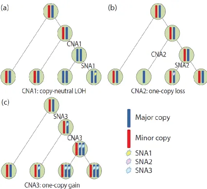
Figure 2.2: Three cases of SNA-CNA phase and order. ... 66

Figure 2.3: Illustration on generating CNA input for Canopy. ... 67

Figure 2.4: Generating new tree topology by local rearrangement. ... 68

Figure 2.5: Inferred phylogenies by Canopy, Clomial and PhyloWGS. ... 70

Figure 2.6: Deconvolution accuracy and clustering quality via simulation studies. ... 71

Figure 2.7: Deconvolution accuracy via simulation studies. ... 72

Figure 2.8: 𝑞𝑚𝑖𝑛 as a measure of deconvolution difficulty from the clonal frequency matrix 𝑃. ... 73

Figure 2.9: Log-likelihood of MCMC sampling with and without pre-clustering step. ... 74

Figure 2.10: Clonal history of transplantable metastasis model MDA-MB-231 with validation by SCP samples. ... 75

ix

Figure 2.12: Canopy’s CNA input to infer phylogeny in the parental cell line and its sublines. ... 80

Figure 2.13: Clonal architecture of breast cancer initial engraftment and passage xenograftment. ... 81

Figure 2.14: Clonal history reconstructed from primary tumor and the relapse genome of leukemia patients. ... 83

Figure 2.15: Clonal history reconstructed from ten spatially separated samples. ... 85

Figure 3.1: Allele-specific transcriptional bursting and gene categorization by single-cell ASE. . 115

Figure 3.2: scRNA-seq protocol and technical variability. ... 116

Figure 3.3: Overview of analysis pipeline of SCALE. ... 117

Figure 3.4: Cell size and cell cycle affects transcriptional bursting. ... 118

Figure 3.5: Modeling of technical variability and parameter estimation. ... 119

Figure 3.6: Gene categorization results on scRNA-seq dataset of mouse blastocyst and human fibroblast cells. ... 120

Figure 3.7: Allele-specific transcriptional kinetics of 7486 genes from 122 mouse blastocyst cells. ... 121

Figure 3.8: Examples of significant genes from hypothesis testing. ... 122

Figure 3.9: Allele-specific kinetic parameter estimation using bursty X-chromosome genes as positive controls. ... 123

Figure 3.10: Testing of bursting kinetics by scRNA-seq and testing mean difference by bulk-tissue sequencing. ... 124

Figure 3.11: Allele-specific transcriptional kinetics of 2277 genes from 104 human fibroblast cells. ... 125

Figure 3.12: Three classes of Poisson-Beta transcription model. ... 126

Figure 3.13: Assessment of moment estimators by simulations studies. ... 128

Figure 3.14: Correlation between allele-specific burst size 𝑠/𝑘𝑜𝑓𝑓, transcription rate 𝑠, and deactivation rate 𝑘𝑜𝑓𝑓. ... 129

x

Figure 3.16: Adjustment of cell size and technical variability leads to more accurate estimation of

allelic bursting kinetics. ... 132

Figure 3.17: Adjustment of cell size and technical variability leads to more accurate estimation of

allelic bursting kinetics. ... 134

Figure 3.18: Histogram repiling method for kinetic parameter estimation with adjustment of

1

CHAPTER 1

NORMALIZATION AND COPY NUMBER VARIATION DETECTION BY WHOLE EXOME

SEQUENCING

1.1 Introduction

Copy number variants (CNVs) are large insertions and deletions that lead to gains and losses of

segments of chromosomes. CNVs are an important and abundant source of variation in the

human genome (1-4). Like other types of genetic variation, some CNVs have been associated

with diseases, such as neuroblastoma (5), autism (6), and Crohn’s disease (7). Better

understanding of the genetics of CNV-associated diseases requires accurate CNV detection.

Traditional genome-wide approaches to detect CNVs make use of array comparative genome

hybridization (CGH) or single nucleotide polymorphism (SNP) array data (8-10). The minimum

detectable size and breakpoint resolution, which are correlated with the density of probes on the

array, are limited. Paired end Sanger sequencing, which is often used as the gold standard

platform for CNV detection, has better resolution and accuracy but requires significant time and

budget investment.

With the dramatic growth of sequencing capacity and the accompanying drop in cost,

massively parallel next-generation sequencing (NGS) offers appealing platforms for CNV

detection. Many current analysis methods are focused on whole genome sequencing (WGS),

which allows for genome-wide CNV detection and finer breakpoint resolution than array-based

approaches (11-15). Whole exome sequencing (WES), on the other hand, has been preferred as

a cheaper, faster, but still effective alternative to WGS in large-scale studies, where the priority

has been to identify disease associated variants in coding regions (16-19).

Due to the biases and artifacts introduced during the exon targeting and amplification

steps of WES, depth of coverage in WES data is heavily contaminated with experimental noise

2

normalization and CNV calling method, CODEX (COpy number variation Detection by EXome

sequencing) (20), to remove biases and artifacts in WES data and produce accurate CNV calls.

Several algorithms have been developed for copy number estimation with whole exome

data in matched case/control settings by either directly using the matched normal (21-23) or

building an optimized reference set (24, 25) to control for artifacts. Other algorithms use singular

value decomposition (SVD) to extract copy number signals from noisy coverage matrices by

removing 𝐾 latent factors that explain the most variance (26-28). This exploratory approach

assumes continuous measurements with Gaussian noise, uses an arbitrary choice of 𝐾, and

doesn’t specifically model known quantifiable biases, such as those due to GC content.

CODEX does not require matched normal controls, but relies on the availability of

multiple samples processed using the same sequencing pipeline. Unlike current approaches,

CODEX uses a Poisson log-linear model that is more suitable for discrete count data. The

normalization model in CODEX includes terms that specifically remove biases due to GC content,

exon length and capture and amplification efficiency, and latent systematic artifacts. We explore

several different statistical approaches for choosing the number of latent factors, and discuss how

one should set this crucial parameter wisely. The power of CODEX and SVD-based approaches

are compared by in silico spike-in studies on the 1000 Genomes Project (29) WES data and show

that CODEX offers higher power in detecting both common and rare CNVs. Also, on WES data

from the 1000 Genomes Project paired with SNP array data from three previous cohort studies on

the same HapMap samples (30-32), CODEX gives higher precision and recall for both rare and

common CNV detection by WES data, as compared to existing methods. CODEX's normalization

and segmentation accuracy is further evaluated through the analysis of the WES data of 222

neuroblastoma matched tumor/blood samples from the TARGET project (33), with a focus on the

well-studied ATRX gene region (33-35). The cross-sample normalization procedure of CODEX,

3

each tumor to its matched normal. The somatic deletions in the ATRX region have a nested

structure, which CODEX was able to recover.

1.2 Results

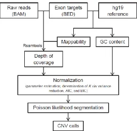
1.2.1 Overview of Analysis Pipeline

Figure 1.1 shows an overview of the analysis pipeline of CODEX. We start with mapped reads

from BAM files (36) that are assembled, sorted, and indexed by the same pipeline, and compute

depth of coverage after a series of quality filtering based on mappability, exon size, and a cutoff

on minimum coverage (see details below). Then, we fit a normalization model based on a

log-linear decomposition of the depth of coverage matrix into effects due to GC content, exon capture

and amplification, and other latent systemic factors. The normalization model produces an

estimated “control coverage” for each exon and each sample, which is the coverage we expect to

see if there is no CNV. Next, the observed coverage for each exon and each sample is compared

to the corresponding estimated control coverage in a Poisson likelihood-based segmentation

algorithm, which returns a segmentation of the genome into regions of homogeneous copy

number. A direct estimate of the relative copy number, in terms of fold change from the expected

control value, can be used for genotyping. CODEX is freely available as a Bioconductor R

package at http://bioconductor.org/packages/CODEX/.

1.2.2 Read Depth Normalization

Due to the extremely high level of systemic bias in WES data, normalization is crucial in WES

CNV calling. CODEX's multi-sample normalization model takes as input the WES depth of

coverage, exon-wise GC content, and sample-wise total number of reads. Specifically, we denote

𝑌 as the coverage matrix with row 𝑖 (1 ≤ 𝑖 ≤ 𝑛) corresponding to the

i

th

𝑗 ≤ 𝑚) to the 𝑗th sample, 𝐺𝐶𝑖 as the GC content for exon 𝑖, and 𝑁𝑗 as the total number of mapped

reads for sample 𝑗. The “null” model, which reflects the expected coverage when there is no

CNVs, is

4

𝜆𝑖𝑗 = 𝑁𝑗𝑓𝑗(𝐺𝐶𝑖)𝛽𝑖exp (∑ 𝑔𝑖𝑘ℎ𝑗𝑘 𝐾

𝑘=1 ),

where 𝑓𝑗(𝐺𝐶𝑖) is the bias due to GC content for exon 𝑖 sample 𝑗; 𝛽𝑖 reflects the exon-specific bias

due to length and capture and amplification efficiency of exon 𝑖; and 𝑔𝑖𝑘ℎ𝑗𝑘 (1 ≤ 𝑘 ≤ 𝐾) are the

th

k

is to estimate the various sources of biases, which can then be used for normalization.

We adopt a robust iterative maximum-likelihood algorithm for estimating the parameters

of the null model. Briefly, in each iteration, we estimate 𝑓(𝐺𝐶) by fitting a smoothing spline of

𝑌 𝑁𝛽exp (𝑔 × ℎ_⁄ 𝑇_{) against the GC content, using the built-in function smooth.spline in R. 𝛽 takes}

the value of the median of each row in 𝑌 𝑁𝑓(𝐺𝐶)exp (𝑔 × ℎ⁄ 𝑇). The latent variables 𝑔𝑖𝑘ℎ𝑗𝑘 (1 ≤

𝑘 ≤ 𝐾) are estimated in the following steps: (i) take known ℎ as covariates, fit 𝑛 Poisson log-linear

regressions with each row of 𝑌 as the response and corresponding row of log (𝑁𝑓(𝐺𝐶)𝛽) as the

fixed offset; (ii) take known 𝑔 as covariates, fit 𝑚 Poisson log-linear regressions with each column

of 𝑌 as the response and corresponding column of log (𝑁𝑓(𝐺𝐶)𝛽) as the fixed offset; (iii) apply

SVD to the row-centered matrix 𝑔 × ℎ𝑇 to obtain the 𝐾 right singular vectors to update ℎ. The third

step ensures the uniqueness and orthogonality of the updated components, which forces the

identifiability of 𝑔𝑖𝑘ℎ𝑗𝑘 (1 ≤ 𝑘 ≤ 𝐾) (37). We fit the Poisson log-linear models with the built-in

function glm in R. See below for details of the maximum-likelihood algorithm. Procedures for

determining 𝐾, the number of latent Poisson factors, is discussed later in 1.4.3 Poisson Latent

Factors and Choice of K.

Initialization

𝛽𝑜𝑙𝑑_{= 1}𝑛_{, 𝑔 = 0}𝑛×𝐾_{, ℎ = 0}𝑚×𝐾_.

Iteration

i. For each sample 𝑗, fit a smoothing spline of [𝑌 𝑁⁄ 𝑗𝛽𝑜𝑙𝑑exp (𝑔 × ℎ𝑇)]_:𝑗 to get 𝑓𝑗(𝐺𝐶).

5

iii. Denote 𝑍 = 𝑁𝑓(𝐺𝐶)𝛽𝑛𝑒𝑤. Apply SVD to row-centered log (𝑌 𝑍⁄ ) to obtain the 𝐾 right

singular vectors and use as ℎ𝑜𝑙𝑑.

a. Fit

n

as fixed offset to obtain updated estimates as 𝑔.

b. Fit 𝑚 Poisson log-linear regressions with 𝑌:𝑗 as response, 𝑔 as covariates, log (𝑍:𝑗) as

fixed offset to obtain updated estimates as ℎ𝑛𝑒𝑤.

c. Center each row of 𝑔 × (ℎ𝑛𝑒𝑤)𝑇 and apply SVD to the row-centered matrix to obtain

the 𝐾 right singular vectors to update ℎ𝑛𝑒𝑤.

d. Repeat steps a to c with ℎ𝑜𝑙𝑑 = ℎ𝑛𝑒𝑤 until convergence to obtain ℎ and 𝑔.

iv. Repeat steps i to iii with 𝛽𝑜𝑙𝑑 = 𝛽𝑛𝑒𝑤 until convergence.

After the normalization procedure, we obtain 𝜆̂ = 𝑁𝛽̂𝑓̂(𝐺𝐶) exp(𝑔̂ × ℎ̂𝑇), which is the

expected “control coverage” in the event where there is no CNV. As described later, the observed

coverage 𝑌 will be compared to the corresponding estimated control coverage 𝜆̂ to test for the

presence of CNVs.

For CNV detection under case-control settings (e.g. tumor with normal) involving

recurrent large chromosomal aberrations, CODEX estimates the exon-wise Poisson latent factor

{𝑔𝑖𝑘} using only the read depths in the control cohort, and then computes the terms {ℎ𝑗𝑘} for the

case samples by regression. This leads to higher sensitivity for detecting variants that are present

only in the case samples. CODEX also includes two modes—“integer” mode that returns copy

numbers as integers for germline CNV detection and “fraction” mode that returns fractional copy

numbers for CNV detection of samples with heterogeneous genetic compositions.

1.2.3 CNV Detection and Copy Number Estimation

Proper normalization sets the stage for accurate segmentation and CNV calling. For germline

CNV detection in normal samples, many CNVs are short and extend over only one or two exons.

6

For longer CNVs and for copy number estimation in tumors where the events are

expected to be large and exhibit nested structure, we propose a Poisson likelihood-based

recursive segmentation algorithm. Let 𝑦𝑠, … , 𝑦𝑡 and 𝜆𝑠, … , 𝜆𝑡 be the raw and estimated control

coverage of the window spanning exon 𝑠 to exon 𝑡. The values 𝜆𝑠, … , 𝜆𝑡 are estimated by the

normalization procedure described in the previous section, but suppressing the sample indicator 𝑗

since we segment each sample separately. A joint cross-sample segmentation, as proposed in

Zhang et al. (38), can also be applied and may yield more accurate results for detection of

germline CNVs. Let 𝑦𝑠:𝑡= ∑𝑡𝑖=𝑠𝑦𝑖 and 𝜆𝑠:𝑡= ∑𝑡𝑖=𝑠𝜆𝑖. The scan statistic we use is max𝑠,𝑡𝑈(𝑠, 𝑡),

where : : : : : : : : :

exp(

)

( , )

sup log

log

(

)

exp(

)

s t

s t

y

s t

s t s t s t

y

s t s t s t

y

U s t

y

y







_























_

_

_

_

_

_



_

_



















The above is the generalized log-likelihood ratio of the alternative model, 𝑦𝑠:𝑡 ~ Poisson(𝜇) with 𝜇

arbitrary, versus the null model, 𝑦𝑠:𝑡 ~ Poisson(𝜆𝑠:𝑡). The copy number estimate for the window is

given by 2𝑦𝑠:𝑡 𝜆⁄ 𝑠:𝑡.

Given the scan statistic, CODEX performs a circular binary segmentation procedure (39)

using 𝑈(𝑠, 𝑡). We further use a modified Bayes Information Criterion (mBIC) to determine the

number of change points 𝑃 in our model (40),

1 0

0

1

1

mBIC( )

log

log(

) (

) log( ),

2

2

P

L

P

P

n

L











_

_















where the first term is the generalized log-likelihood ratio for the model with 𝑃 change points

versus the null model with no change points; 𝜏𝜌 (1 ≤ 𝜌 ≤ 𝑃) is the 𝜌th change point, 1 = 𝜏0<

𝜏1< ⋯ < 𝜏𝑃< 𝜏𝑃+1= 𝑛; 𝑛 is the number of exons. We report the segmentation with 𝑃̂ =

𝑎𝑟𝑔𝑚𝑎𝑥𝑃𝑚𝐵𝐼𝐶(𝑃). Compared with algorithms based on HMM such as XHMM (28) and

EXCAVATOR (25), CODEX doesn't require the user to pre-specify unknown parameters, such as

expected distance between exons, exon-wise CNV rate, and average number of exons in a CNV.

7

many cases have to be chosen arbitrarily. Post-segmentation, CODEX outputs an estimate of the

relative copy number in terms of fold change from the expected control coverage, rather than a

binary categorization of deletion and duplication as in CoNIFER (26) and XHMM (28).

1.2.4 Calling Germline Variations from HapMap Samples

To examine the accuracy of CODEX and to illustrate its application, we use a publicly available

WES data set from the 1000 Genomes Project Phase 1 release (29) containing 90 healthy

individuals. 46 samples are sequenced at the Washington University Genome Sequencing Center

(captured by HSGC VCRome) and 44 at the Baylor College of Medicine (captured by SureSelect

All Exon V2). All samples have Omni and Axiom genotypes and have more than 70% of exome

targets covered to 20x or more. Sex is well balanced (44 males and 46 females) and population

(40 Utah residents with northern and western European ancestry (CEU), 24 Japanese people

from Tokyo (JPT), and 26 Yoruba people from Ibadan (YRI)) adds a potential source of latent

variation.

Effectiveness of normalization procedure

We first examine the effectiveness of CODEX’s proposed normalization model on the 1000

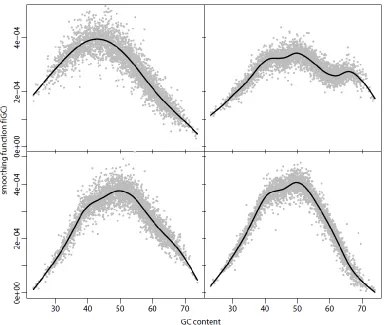
Genomes Project WES data set (29). Previous studies have shown that read depth has a

unimodal relationship with GC content—regions with high or low GC content tend to have

decreased read depth (41). In our smoothed estimates of 𝑓𝑗(𝐺𝐶), we find that most but not all

samples have a unimodal shape for this function. We show the predicted values of 𝑓𝑗(𝐺𝐶) for 4

typical samples in Figure 1.2. Interestingly, we found that some samples have estimates with

multiple peaks in 𝑓𝑗(𝐺𝐶), which suggests that a parametric functional form assuming unimodality

may be too simplistic. Comparing across samples, we see that the function 𝑓𝑗(𝐺𝐶) changes in

shape and not just by a scaling factor. Therefore, the GC content bias is not linear across

samples and thus cannot be fully captured by linear latent factor models. This motivates the

8

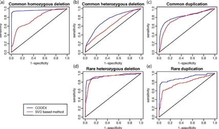
We further compare the normalization result of CODEX against that of SVD based

method using array-based CNV calls from the International HapMap Consortium (30) on the

same samples we analyze. For different categories of CNV events, namely, homozygous

deletions, heterozygous deletions, and duplications, we use direct thresholding of log (𝑌 𝜆̂⁄ ) to

draw receiver operating characteristic (ROC) curves of our model, where 𝜆̂ is the estimated

control coverage from CODEX’s normalization procedure. The ROC curves for SVD-based

normalization are drawn by thresholding on the residuals obtained by subtracting the first 𝐾 PCs

from the original read depth 𝑌. Analysis is carried out for each of the following category of events

separately: common homozygous deletion, common heterozygous deletion, common duplication,

rare heterozygous deletion, and rare duplication (Figure 1.3). There are no rare homozygous

deletions as all of the rare deletions from the HapMap CNV call set are present in only

heterozygous form. We see that CODEX’s normalization procedure leads to a better

signal-to-noise ratio for both common and rare CNVs, and for both deletions and duplications (Figure 1.3).

Accuracy of CNV calling

We next compare the accuracy of CODEX to existing approaches that are designed for

population-based CNV calling. These programs include CoNIFER (26), XHMM (28), and

EXCAVATOR (25) in its “pooling” mode, for which we added four additional samples as controls.

The number of calls made by each program on each chromosome sample, broken down

into common and rare calls, is shown in Table 1.1. Globally, CODEX detects twice as many CNV

events as XHMM does and nearly 10 times as many as CoNIFER does, while EXCAVATOR and

CODEX have comparable number of calls. CoNIFER detects the fewest CNVs in total, which

agrees with comparisons against EXCAVATOR made in Magi et al. (25). Since CoNIFER does

not automatically choose the number of PCs, we fix the number of PCs filtered out by CoNIFER

at 4, agreeing with the selection made by XHMM so as to make the two SVD-based programs

comparable. The choice of 4 PCs in normalization should not account for the low number of calls

9

contributed variance to be still significantly decreasing at 4, indicating that the choice of 4 is

conservative. A large proportion of XHMM and CoNIFER calls are rare (<5%) variants—52.46%

(501/955) and 83.07% (157/189) respectively. Despite the bias in sensitivity of XHMM and

CoNIFER towards rare variants, CODEX detects even more rare CNVs in total as well as

proportionately more common ones. Notably, the number of latent factors

K

is for most chromosomes one less than the number of PCs excluded by XHMM across the

genome. Furthermore, CODEX and XHMM tends to detect shorter CNVs compared to CoNIFER

and EXCAVATOR in units of both kb (Figure 1.4a) and exon (Figure 1.4b).

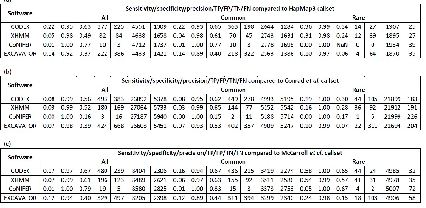
We assess the CNV calls made by the four methods by comparing to calls reported by

the International HapMap Consortium (30), McCarroll et al. (31), and Conrad et al. (32) in the

same 90 HapMap samples. The International HapMap 3 Consortium produced a clean CNV call

set by merging and utilizing probe-level intensity from both Affymetrix and Illumina arrays,

containing 856 copy number polymorphisms (CNPs) with a 99.0% mean call rate and 0.3%

Mendelian inconsistency (30). Separately, McCarroll et al. developed a map consisting of 1320

CNVs at 2-kb breakpoint resolution by joint analysis of Affymetrix SNP array, array CGH (42) and

fosmid end-sequence-pair data (31, 43). The third source of validation we use is the call set from

Conrad et al., who used Nimblegen tiling oligonucleotide arrays to generate a map of 11,700

CNVs greater than 443 base pairs, of which 8,599 have been validated independently (32). The

genotyped CNPs from these three cohort studies that overlap with exon regions (73, 123, and

377 in total respectively) are used as “validation set” to assess sensitivity and specificity of the

four methods compared in Table 1.1. Figure 1.5 shows the precision and recall rates (precision is

the proportion of calls made by the program that overlap with validation set, and recall is the

proportion of the CNVs in validation set that are called.) The different programs vary

considerably in precision and recall rate. CODEX has the highest F-measure (harmonic mean of

precision and recall) for both common and rare CNVs. XHMM performs well in detecting rare

10

against calls from the International HapMap Consortium (Figure 1.5a) and McCarroll et al. (Figure

1.5c) but gives poor results against Conrad et al. (Figure 1.5b). Furthermore, the high precision of

CoNIFER come with significant sacrifice on recall. See Table 1.2 for detailed comparison results

based on the three SNP array metrics.

1.2.5 Sensitivity Assessment with Spike-in Study

We next conduct an in silico spike-in study to assess the sensitivity of the different methods at

varying population frequencies. Starting with the WES data from chromosome 20 of the 𝑚 = 90

HapMap samples analysed in the previous Section, we spike CNV signals in to

copy-number-neutral regions. We define a region to be copy-number-copy-number-neutral if it doesn’t overlap with CNV calls

made by CODEX, XHMM, EXCAVATOR, and CoNIFER nor with previously reported CNV

regions by DGV (http://dgv.tcag.ca/dgv/app/) and dbVar (http://www.ncbi.nlm.nih.gov/dbvar/). Of

the 3966 exon targets on chromosome 20, 1035 pass this criterion for copy-number-neutral. We

consider only heterozygous deletions of two different lengths (5 and 10 exons) and varying

population frequencies 𝑝 ∈ {5%, 10%, … ,95%}. We focus on heterozygous deletions because (i)

homozygous deletions are easily detectable by all methods; (ii) heterozygous deletions with

frequency 𝑝 in the population have exactly the same detection accuracy as duplications with

frequency 1 − 𝑝. Specifically, for deletions with population frequencies greater than 50%,

copy-number-neutral states are reported as duplications whereas deletions are reported as normal

events, since all copy number events are defined in reference to a population average. Events

are centered at every hundredth exon and 𝑚 × 𝑝 samples are randomly chosen to be carriers. To

generate CNV signals for heterozygous deletions, we reduce the raw depth of coverage for exons

spanned by the CNV from 𝑦 to 𝑐

2× 𝑦, where 𝑐 is sampled from a normal distribution with mean 1

and standard deviation 0.1.

We apply CODEX to these spike-in data sets and compare it to SVD-based normalization

followed by HMM-based segmentation. For the latter, we remove the first 𝐾 principal components

11

separately. The 𝑧-scores are then segmented by a HMM whose parameters are set as the default

values in XHMM. The specificity of both approaches is controlled to be higher than 99%. The

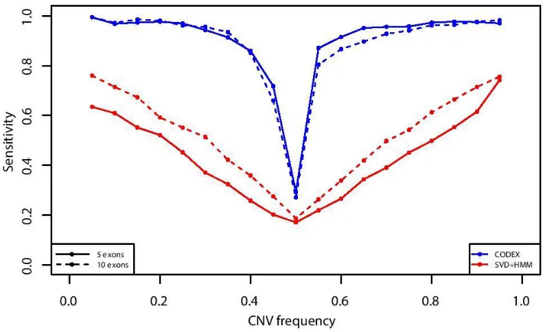
sensitivities for short CNV (5 exons) and long CNV (10 exons) at different population frequency

levels are shown in Figure 1.6. We see that both approaches attain high sensitivity for rare

CNVs, and both have decreased sensitivity for common CNV events. The sensitivity of CODEX is

higher than that of the existing approach for both rare and common variants (Figure 1.6). For

CNV events with frequencies around 50%, both methods have the lowest power due to the fact

that the CNV signals are falsely filtered out by a sample-wise latent factor (Figure 1.6). Also,

shorter CNV events are more often missed by the SVD approach whereas CODEX has

comparable sensitivity for short and long variants at this scale (Figure 1.6).

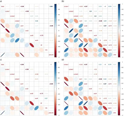
To gain a better understanding of what the latent factors in CODEX and SVD-based

methods are capturing, we show in Figure 1.7 the correlation of the latent factors to measurable

quantities. The exon-wise latent factors in both models and the estimated value of 𝛽 in CODEX

are compared to GC content, mean exon coverage, and true copy number. The sample-wise

latent factors in both models are compared to center, batch, population, and total coverage (𝑁).

Based on these correlations, we make the following observations: First, mean exon coverage,

represented by the pseudo-reference sample {(∏𝑚𝑣=1𝑌𝑖𝑣)1 𝑚⁄ : 1 ≤ 𝑖 ≤ 𝑛}, is captured by 𝛽 in

(correlation coefficient 0.99) in CODEX and the first exon-wise PC in SVD (correlation coefficient

-0.98). Exon length and capture and amplification efficiency are confounded in this exon-specific

bias and there is no way, nor any need, to estimate these individual quantities separately.

Second, GC content is correlated with the third exonwise PC in SVD (correlation coefficient

-0.75). CODEX specifically models the GC content bias for each sample by the term {𝑓𝑗(𝐺𝐶): 1 ≤

𝑗 ≤ 𝑚}, and as we show later, the bias cannot be fully captured by a linear PC. Third, a CNV that

is more frequent in the population has higher absolute correlation between copy number state

and the exon-wise latent factors in both CODEX (-0.22) and SVD (0.57). This is why sensitivity is

12

batch, are captured by sample-wise latent factors in both CODEX (correlation coefficient -1 and

0.74) and SVD (correlation coefficient 0.97 and -0.71). In this data set, population doesn’t seem

to be captured by any of the top latent factors.

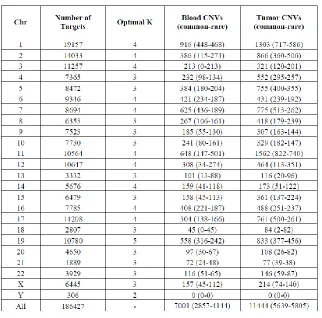
1.2.6 Analysis of Whole Exome Sequencing of Neuroblastoma

We also analyze a WES data set consisting of 222 paired tumor/normal (blood leukocyte)

samples of individuals older than 18 months of age at diagnosis with stage-4 neuroblastoma from

the TARGET Project (33). WES of native and whole genome amplified DNA of ~33Mb regions

yields a 124X average coverage, with 87% of bases suitable for mutation detection (33). Our

discussion here focuses on the well characterized ATRX gene region (33-35). The TARGET

Project reported recurrent focal deletions with a complex nested structure spanning the ATRX

gene. Since there are matched normal samples for this study that have also been sequenced by

the same technology, the TARGET calls were made by comparing each tumor sample to its

matched normal. This allows us to compare the effectiveness of CODEX’s normalization model

to that of taking a log ratio to the matched normal coverage. Also, focusing on this well

characterized region allows us to demonstrate in accuracy of CODEX for handling recurrent

complex nested events.

The RPKM (reads per kilo bases per million reads) for each exon and each sample are

plotted in Figure 1.8a. The RPKM profiles are very noisy and do not show any clear decrease in

this region in any of the samples, highlighting the need for normalization. For comparison, we

also show the TARGET Project's initial analysis, which reported 16 multiexon deletions within

ATRX by comparing tumor to matched normal samples (33). Specifically, we repeat their analysis

by thresholding the log2-ratio of RPKM in tumor to RPKM in normal samples, illustrated in Figure

1.8b. Figure 1.8c shows the normalized intensities given by CODEX, which detects 18 samples

with somatic focal deletions. We also apply XHMM to the tumor data set and detect 14 samples

13

Of the 18 samples with somatic deletions detected by CODEX, three are also called by

the TARGET Project but missed by XHMM; one is detected by XHMM and CODEX with exactly

the same breakpoints but is missed by the Target Project; one is uniquely called by CODEX

(Table 1.3a). The sample uniquely called by CODEX is a small deletion that overlaps significantly

with deletions called in other samples. Detailed CNV calling and genotyping results by each

method are in Table 1.3b-d and the genome-wide blood and tumor CNV events discovered by

CODEX are summarized in Table 1.4. The comprehensive analysis results will be published

separately.

It is clear by visual comparison of Figure 1.8c to Figure 1.8b and Figure 1.8b that the

read depth normalization method within CODEX gives better signal to noise ratio than the SVD

based normalization method in XHMM (note the difference in range of the y-axes) and also better

than the commonly prescribed method of normalizing to matched normal controls. This illustrates

that by borrowing information across a large cohort, the estimated control coverage of 𝜆̂ from our

normalization model is more effective in capturing the biases in whole exome sequencing than

the matched normal. Whereas the matched normal sample is important to distinguish between

germline and somatic variants, CODEX's normalization procedure can be used in case of

unavailability of blood samples or contamination of blood samples from circulating tumor cells.

When matched normal is available, somatic status can be determined by comparing CODEX calls

in tumor to those in normal. This example also shows that CODEX's segmentation algorithm

performs well in detecting multiexon CNVs with a nested structure, and that it successfully

detected a rare CNVs (18/222=8.11%) in a clinical setting.

1.3 Discussion

Here we propose CODEX, a normalization and CNV detection method for WES data. CODEX

includes a normalization model with non-parametric functional terms for GC content and Poisson

latent factors for biases that are not directly quantifiable. We show that both parts of the

14

Poisson likelihood model based on the control coverage 𝜆̂ estimated during the normalization

step. CODEX can be applied to both normal and tumor genome analysis.

We show through several data sets that CODEX's multi-sample normalization procedure

offers higher sensitivity and specificity for detection and genotyping of both common and rare

CNVs. The distinguishing features of CODEX compared to existing methods are: (i) CODEX

doesn’t require matched normal samples as controls for normalization; (ii) The Poisson log-linear

model fits better with the WES count data than SVD approaches; (iii) Dependence on GC content

is modelled by a flexible nonparametric function in CODEX allowing it to capture non-linear

biases; (iv) CODEX implements the BIC criterion for choosing the number of latent variables,

which gives a conservative normalization on simulated and real data sets; (v) Compared to

HMM-based segmentation procedures, the segmentation procedure in CODEX is completely

off-the-shelf and doesn’t require large relevant training set; (vi) CODEX estimates relative copy number,

which can be converted to genotypes by thresholding, rather than broad categorizations (deletion,

duplication, and copy number neutral states).

We carry out simulation studies by spiking in CNV signals to WES read depth data from

copy-number-neutral regions. We show that CODEX has higher power compared to SVD based

method followed by HMM, although both methods suffer from common CNV events. We also

investigate the nature of the exon- and sample-wise terms and Poisson factors in CODEX, PCs

extracted by SVD, and other directly known biases and artifacts. We show that PCs from SVD

obtained by unsupervised learning are correlated by the terms specifically modelled and

quantified by CODEX and that the GC content correlates with one PC from SVD with correlation

coefficient -0.75, which, again, is specifically modelled by CODEX. Developing a robust method

that can detect common CNVs from background noise with high sensitivities may be a future

direction to get focused on.

We compare CODEX’s performance against direct calling results from other existing

15

comparing CNV calls by WES against three gold standard SNP array CNV call sets. Since

CoNIFER and EXCAVATOR detect a significant proportion of CNVs with lengths greater than 200

kb whereas CODEX and XHMM return much shorter CNVs (Figure 1.4), we don’t exclude any

CNV calls by SNP arrays so as to get more “reliable” gold standards as does Fromer et al. (28),

despite the fact that array based methods, when compared to next-generation sequencing, don’t

have as good resolutions. This might explain why the overall sensitivity/recall rates are no larger

than 0.6 for all methods (Figure 1.5, Table 1.2). Another possible explanation lie in that due to the

discrete nature of WES data, read depth is used as the only inference to detect CNVs, which has

only exon-level resolution and thus lower power in detecting short CNVs compared to split-read

and paired-end-mapping methods developed for WGS. Despite the limitations, WES has been

used and is still being used as a preferred method of choice for large-scale studies.

With a clinically relevant example on detecting rare somatic CNVs within ATRX

associated with neuroblastoma, CODEX is shown to be applicable to a wide range of study

designs for CNV detection using WES data. Specifically, we show that CODEX doesn’t require

matched normal controls for normalization and is able to detect previously reported CNVs within

tumor samples more accurately compared to SVD-based method. Matched blood samples, when

available, can be used to distinguish somatic CNVs from germline ones. However, under most

circumstances, the normal samples are often unavailable, incomplete, or unmatched, which

drives the need for normalization using cases only. The genome-wide CNV results based on this

data set are available and will be compared against other metrics (matched microarrays,

whole-genome sequencing, RNA-sequencing, etc.) and validated on bench. The comprehensive

analysis results will be published elsewhere.

1.4 Methods

1.4.1 Sample Selection and Target Filtering

To have as much sample- and exon-wise homogeneity as possible and to make sure that our

16

selection and target filtering strategy before applying our proposed normalization method to the

read depth data. Specifically, for reducing artifacts, we recommend that all of the samples be

sequenced by the same platform. We further filter out exons that: (i) have extremely low coverage

(median read depth across all samples less than 20, which mostly reflect capture failure); (ii) are

extremely short (less than 20 base pairs); (iii) are hard to map (mappability less than 0.9); (iv)

have extreme GC content (less than 20% or greater than 80%). These default thresholds for

quality control (QC) are recommended but are also user-tuneable and thus can be adapted to

different sequencing protocols. We show in Table 1.1 that with the above QC thresholds, 9.74%

of exon targets are excluded in the data. Details on computation of GC content, mappability, and

depth of coverage are provided in 1.4.2 Depth of Coverage, GC Content, and Mappability.

1.4.2 Depth of Coverage, GC Content, and Mappability

Depth of coverage for each exon is computed as the number of reads (with mapping quality

greater than a user-defined threshold) that overlap with the exon. To calculate the exonic

mappability, we first construct consecutive reads that are one base pair (bp) apart along the exon.

The length of the reads is set to be the same as that from the sequencing technology and the

sequences are taken from the hg19 reference. We then find possible positions across the

genome that the reads can map to allowing for a default number of mismatches (2 for the 1000

Genomes Project data set in our study which has read 100). Finally we compute the mean of the

probabilities that the overlapped reads map to the target places where they are generated and

use this as the mappability of the exon.

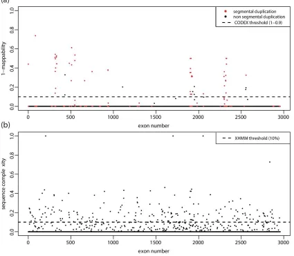
We compare our computed exonic mappability with the number of overlapped segmental

duplications from the Segmental Duplication Database. Results show that not all segmental

duplication regions are hard to map and thus it is not wise to directly filter out exons that overlap

with segmental duplications (Figure 1.9a). As a comparison, we also compute the sequence

complexity—percentage of bases within exons soft masked by RepeatMasker

17

which is the filtering strategy adopted by XHMM. It turns out that not only XHMM has an overly

stringent threshold on sequence complexity/mappability (Figure 1.9b), but also it includes other

outlier removal steps, such as removing samples with coverage that are empirical outliers,

filtering out targets with a standard deviation of PCA-normalized z-score greater than 30, etc.

These additional empirical ways of excluding samples and targets might treat true signals as

outliers and remove them.

1.4.3 Poisson Latent Factors and Choice of K

Some sources of bias in whole exome sequencing can be directly measured (GC content,

mappability, and exon size). However, there are other unmeasurable sample- and target-specific

biases that are amplified during the library preparation and sequencing experiment. The latent

Poisson factors {𝑔𝑖𝑘} and {ℎ𝑗𝑘} are designed to capture and decompose these unobserved

systemic bias in a log-additive manner. Such latent factor models have been shown to be

effective in the analysis of microarray data (44-47), and have also recently been applied to NGS

data. Both CoNIFER (26) and XHMM (28) use latent factor models to remove systemic bias, but

their models assume continuous measurements with Gaussian noise structure, while CODEX is

based on a Poisson log-linear model, which is more suitable for modeling the discrete counts in

WES data, especially when there is high variance in depth of coverage between exons. The

latent factor terms in the normalization model resemble those used in Lee et al. (37) for

microRNA profiling. In particular, the identifiability constraints in Lee et al. also apply to our case,

and our iterative maximum-likelihood estimation procedure ensures identifiability.

A common downfall of latent factor models is that true CNV signals may correlate with

and influence the top 𝐾 latent factors. Thus, the number of latent factors, 𝐾, is a crucial

parameter. If 𝐾 is chosen to be too large, some bona fide CNV signals, especially those for

common CNVs, will be dampened during normalization. On the other hand, if 𝐾 is too small,

residual artifacts will remain and inflate the type I error rate. CoNIFER (26) adopts a common

18

plot with the number of components on the X-axis and the corresponding contributed variance on

the Y-axis. If there is an “elbow” in the scree plot, then 𝐾 is chosen at the position of the elbow

(Figure 1.10a). However, in most cases there is no detectable elbow, which is why many existing

methods arbitrarily set the value of 𝐾. XHMM (28) removes components with variance 0.7 𝑚⁄ or

higher, where 𝑚 is the number of components (samples) and 0.7 is a user-tuneable parameter

arbitrarily set as default.

We apply two additional statistical procedures of choosing this crucial model tuning

parameter: Akaike information criterion (AIC, Figure 1.10b) and Bayes information criterion (BIC,

Figure 1.10c).

AIC = 2 ln(𝐿) − 2𝑘

BIC = 2 ln(𝐿) − 𝑘 ln(𝑛)

where 𝐿 is the likelihood for the estimated model, 𝑘 is the number of parameters in the model,

and 𝑛 is the number of data points. Both criteria reward goodness of fit with a penalty term that is

an increasing function of the number of parameters in the model. AIC penalizes the number of

parameters less strongly than does BIC, and thus the model chosen by AIC removes more latent

factors than that chosen by BIC. CODEX reports all three statistical metrics (AIC, BIC,

percentage of variance explained) and uses BIC as the default method to determine the number

of 𝐾. Since false positives can be screened out through a closer examination of the

post-segmentation data, whereas CNV signals removed in the normalization step cannot be

recovered, CODEX opts for a more conservative normalization that, when in doubt, uses a

19

Figure 1.1: A flowchart outlining the procedures of CODEX in normalizing WES read depth

and calling CNV. The first step is computing GC content, mappability, and depth of coverage

using Rsamtools with QC measures. The multi-sample normalization model by CODEX is then

applied to remove biases and artifacts introduced by GC content, exon targeting and amplification

efficiency, and latent systemic artifacts. The Poisson likelihood-based segmentation algorithm

20

Figure 1.2: Predicted values of 𝒇(𝑮𝑪) for 4 samples from the 1000 Genomes Project data set. Most patterns agree with previous observations that read depth has a unimodal relationship

with GC content. However, dual modality is also observed. Furthermore, the function changes in

21

Figure 1.3: ROC curves of read depth normalization by CODEX and SVD-based method.

Gold standard is taken from the International HapMap Consortium SNP array CNV call set. The

input for CODEX is the log2-ratio of the original read depth 𝑌 versus the estimated control

coverage 𝜆̂; the input for SVD-based method is the residual obtained by subtracting the principal

components from the original read depth 𝑌. For common CNVs shown in (a), (b), and (c), CODEX

performs significantly better since SVD-based methods are optimized for rare CNV detection; for

rare CNVs shown in (d) and (e), the two methods tend to have similar power for rare

heterozygous deletions whereas CODEX performs better in detecting rare duplications. Of the 90

samples we analyze, there is no rare heterozygous deletion from the HapMap call set that we can

22

Figure 1.4: Lengths of CNV calls by CODEX, XHMM, CoNIFER, and EXCAVATOR. Genomics

lengths of CNVs (a) and number of exons in CNV regions (b) are compared across four different

methods. CODEX and XHMM detects more short CNVs whereas CoNIFER and EXCAVATOR

23

Figure 1.5: Assessment of CNV calls on the 1000 Genomes Project by array-based

methods. CNV calls by CODEX, XHMM, CoNIFER, and EXCAVATOR are validated against

genotyping calls from International HapMap Consortium (a), Conrad et al. (b), and McCarroll et al.

(c). CODEX returns well-balanced precision and recall rates with highest F-measures (grey

contours shown harmonic means of precision and recall rates) among all methods for detection of

24

Figure 1.6: Power analysis of CODEX and SVD-based method on simulation data set.

Sensitivities are obtained by averaging results from 10 simulations. Both methods suffer from “common” CNV events (CNVs with frequencies around 50%). When CNV frequency exceeds

50%, deletions and copy-neutral states are detected as copy-neutral states and duplications

instead, which recovers the sensitivities. CODEX performs better compared to SVD-based

25

Figure 1.7: Correlation matrix plot of biases and artifacts shown in both exon-wise and

sample-wise fashion. 𝛽, exon-wise latent factors, GC content, copy-number state, and pseudo-reference genome are interrogated in (a) and (c). Sample-wise latent factors, total number of

reads per sample, sequencing centers, batch effects, and population are shown in (b) and (d). (a)

and (b) are for spike-in CNV events with frequency 0.1 and (c) and (d) are for spike-in CNV

events with frequency 0.4. 𝛽 and first exon-wise PC in SVD highly correlate with

pseudo-reference genome. GC content is correlated with the third exon-wise PC in SVD with correlation

coefficient -0.75. Copy-number states show higher correlation for spiked-in CNVs with higher

27

Figure 1.8: Detection of rare somatic deletions within ATRX by WES of 222 neuroblastoma

matched tumor/blood samples. Location of ATRX is shown as blue bars in c and d. (a) RPKM

computed from the tumor samples. There is no clear visual indication of presence of somatic

CNVs from these raw quantities. (b) Log2-ratio of tumor versus blood read depth. Initial analysis

by the TARGET Project did careful inspection of these values and discovered 17 samples with

focal deletions. (c) log2-ratio of the original tumor read depth 𝑌 versus the estimated control

coverage 𝜆̂ (model fitted on tumor data set only) by CODEX. Poisson likelihood-based

segmentation algorithm by CODEX discovers 18 samples (red bars) with somatic deletions that

exhibit a nested structure across samples. The 4 samples that are called by CODEX but not by

XHMM are colored in red in the embedded window. (d) XHMM's direct output: z-scores

normalized by principal component analysis. The HMM calling algorithm by XHMM detects 14

28

Figure 1.9: Filtering strategies on mappability and sequence complexity by CODEX and

XHMM. Computation results from chromosome 22 are shown with filtering thresholds in dashed

lines. (a) Mappability computed by CODEX. Exons that overlap with previously reported

segmental duplications are marked in red. (b) Sequence complexity used in pre-filtering step by

29

Figure 1.10: Choice of 𝑲, number of latent Poisson factors. Remaining variance in the read

depth data (a), AIC (b), and BIC (c) are used as three different metrics, which yield similar models

with 𝐾 optimally set at 3 or 4. Each line represents result of one chromosome. Suggested 𝐾 is

30

Table 1.1: CNV call sets information on the 1000 Genomes Project WES data set. Number of

exon targets before and after QC procedure is shown. CNVs detected by CODEX, XHMM,

CoNIFER, and EXCAVATOR are shown and are further categorized into common and rare ones

(common-rare in parentheses). Number of latent factors (𝐾) and principal components (PCs) are

shown for latent factor models: default values from CODEX and XHMM are adopted; number of

PCs for CoNIFER is chosen at 4 so that it is conservative by the scree plot and is comparable to

31

Table 1.2: Sensitivity, specificity, and precision rate of CNV calls by CODEX, XHMM,

CoNIFER, and EXCAVATOR. The plot of precision and recall rates are shown in Figure 5. Three

“gold-standard” CNV metrics are adopted from (a) International HapMap Consortium, (b) Conrad et al., and (c) McCarroll et al.. CODEX and XHMM performs better in detecting rare CNVs

compared to common ones, with CODEX having the highest F-measure among all methods

32

(a)

33

(c)

(d)

Table 1.3: Somatic deletions within ATRX region detected using WES data of

neuroblastoma patients. (a) Summary of deletions detected by tumor/normal threshold,

CODEX, and XHMM with break-point and length information. Of the 18 samples detected by CODEX, 16 samples overlap with the matched tumor blood analysis result; 14 and all of XHMM’s

CNV events are detected; one sample is uniquely called. Breakpoints may differ slightly between

different methods but are within reasonable limits. (b) Deletions detected by thresholdhing log2

-ratio of tumor RPKM to blood RPKM. (c) Deletions detected using tumor samples only by

34

Table 1.4: Genome-wide CNVs detected by CODEX of the neuroblastoma data set. Blood