IMPACT OF EDGE DETECTION ALGORITHM IN IMAGE PROCESSING

1514 |

P a g e

IMPACT OF EDGE DETECTION ALGORITHM IN

IMAGE PROCESSING

C.A.Md. Zameer

1

, A.Viswanthan

2

, A.A.Khadar Maideen

3

1, 2

Assistant Professor,

Department of Computer Science, Islamiah College[Autonomus],

Thiruvalluvar University, vaniyambadi, (India)

3

Research Guide & Associate Professor,

Department of Computer Science, Islamiah College

[Autonomus], Thiruvalluvar University, vaniyambadi,(India)

ABSTRACT

The basic pitfall in Image analysis is Edge detection. Edge characteristics and boundaries are useful information in Image segmentation. Edges play an important role in many applications of image processing, in particular for machine vision systems that analyze scenes of man-made objects under controlled illumination conditions. Image edge detection is a process of locating the edge of an image which is important in finding the approximate absolute gradient magnitude at each point of an input grayscale image. The problem of getting an appropriate absolute gradient magnitude for edges lies in the method used. This paper aims at throwing light on the various edge detection methods. The various Edge detection methods are applied on the sample data. The pros and cons of them are summarized.

Keywords:

Image analysis, Edge Detection operator, Gray scale input.

I. INTRODUCTION

Image processing is important in modern data storage and data transmission especially in progressive

transmission of images, video coding(teleconferencing), digital libraries, and imagedatabase, remote

sensing. It has to do with manipulation of images done by algorithm to produce desired images . Digital Signal

Processing (DSP) improve the quality of images taken under extremely unfavorable conditions in several

ways: brightness and contrast adjustment, edge detection, noise reduction, focus adjustment,

motion blur reduction etc. The advantage is that image processing allows much wider range of algorithms to

be applied to the input data in order to avoid problems such as the build-up of noise and signal distortion

during processing.[1,2,3]. With the fast computers and signal processors available in the 2000's, digital image

processing became the most common form of image processing and is general used because it is not only the

most versatile method but also the cheapest. The process allows the use of much more complex algorithms for

image processing and hence can offer both more sophisticated performances at simple tasks .Detection of edges

in an image is a very important step towards understanding image features. Edges consist of meaningful features

and contained significant information. It‟s reduce significantly the amount of the image size and filters out

1515 |

P a g e

II.TYPES OF EDGE DETECTION

An edge operator is a neighborhood operation which determines the extent to which each pixel's

neighborhood can be partitioned by a simple arc passing through the pixel where pixels in the

neighborhood on one side of the arc have one predominant value and pixels in the neighborhood on the other

side of the arc have a different predominant value. Usually gradient operators, Laplacian operators,

zero-crossing operators are used for edge detection. The gradient operators compute some quantity related to

the magnitude of the slope of the underlying image gray tone intensity surface of which the observed image

pixel values are noisy discretized sample. The Laplacian operators compute some quantity related to the

Laplacian of the underlying image gray tone intensity surface. The zero-crossing operators determine whether

or not the digital Laplacian or the estimated second direction derivative has a zero-crossing within the pixel.

Gradient based Roberts, Sobel and Prewitt edge detection operators, Laplacian based edge detector and Canny

edge detector.

The common methods that are used for edge detection are:



Gaussian Method



Gradient Method (First Order Derivate)



Laplacian Method(Second Order Derivative)

2.1 Gradient Method

In this edge detection method the assumption is that edges are the pixels with a high gradient. A fast rate of

change of intensity at some direction given by the angle of the gradient vector is observed at edge pixels. An

ideal edge pixel and the corresponding gradient vector is shown. At the pixel, the intensity changes from 0 to

255 at the direction of the gradient. The magnitude of the gradient indicates the strength of the edge. If we

calculate the gradient at uniform regions we end up with a zero vector which means that there is no edge pixel.

In natural images we usually do not have the ideal discontinuity or the uniform regions as in the figure and we

process the magnitude of the gradient to make a decision to detect the edge pixels. The simplest processing is

applying a threshold. If the gradient magnitude is larger than the threshold we decide that the corresponding pixel

is an edge pixel. An edge pixel is described using two important features:



Edge strength, which is equal to the magnitude of the gradient.



Edge direction, which is equal to the angle of the gradient.

The gradient for the ideal continuous image is estimated using some operators. Among these operators

"Roberts, Sobel and Prewitt" are the commonly used.

2.2 Roberts Operator

The Roberts cross operator provides a simple approximation to the gradient magnitude:

1516 |

P a g e

Fig. 1 Roberts Operator

where Gx and Gy are calculated using the following mask.

As with the previous 2 x 2 gradient operator, the differences are computed at the interpolated point [i + 1/2, j +

1/2]. The Roberts operator is an approximation to the continuous gradient at this interpolated point and not at

the point [i, j] as might be expected[5].

2.3 Sobel Operator

A way to avoid having the gradient calculated about an interpolated point between pixels is to use a 3 x 3

neighborhood for the gradient calculations. Consider the arrangement of pixels about the pixel [i, j] The

Sobel operator is the magnitude of the gradient computed by:

where the partial derivatives are computed by:

with the constant c = 2.

Like the other gradient operators, Sx and Sy can be implemented using

convolution masks:

Fig. 2: Sobel Operator

this operator places an emphasis on pixels that are closer to the center of the mask. The Sobel operator is one of

the most commonly used edge detectors. The labeling of neighborhood pixels used to explain the Sobel and

Prewitt operator.

Fig.3: Gradient Vector

2.4 Prewit Operator

The Prewitt operator uses the same equations as the Sobel operator, except that the constant c = 1. Therefore:

1517 |

P a g e

Unlike the Sobel operator, this operator does not place any emphasis on pixels that are closer to the center

of the masks

2.5 Laplacian Based Edge Detection

The edge points of an image can be detected by finding the zero crossings of the second derivative of the

image intensity. The idea is illustrated for a 1D signal in Figure 5.3.1. However, calculating 2nd derivative

is very sensitive to noise. This noise should be filtered out before edge detection. To achieve this,

“Laplacian of Gaussian” is used. This method combines Gaussian filtering with the Laplacian for edge

detection. In Laplacian of Gaussian edge detection there are mainly three steps:



Filtering,



Enhancement,



Detection.

Gaussian filter is used for smoothing and the second derivative of which is used for the enhancement step. The

detection criterion is the presence of a zero crossing in the second derivative with the corresponding large peak

in the first derivative.

In this approach, firstly noise is reduced by convoluting the image with a Gaussian filter. Isolated noise

points and small structures are filtered out. With smoothing; however; edges are spread. Those pixels, that have

locally maximum gradient, are considered as edges by the edge detector in which zero crossings of the second

derivative are used. To avoid detection of insignificant edges, only the zero crossings, whose corresponding

first derivative is above some threshold, are selected as edge point. The edge direction is obtained using the

direction in which zero crossing occurs[7,8].

The output of the Laplacian of Gaussian (LoG) operator; h(x,y); is obtained by the convolution operation:

where

is commonly called the Mexican hat operator.

Fig.5: Mexican hat operator

In the LoG there are two methods which are mathematically equivalent:

1518 |

P a g e



Convolve the image with the linear filter that is the Laplacian of the Gaussian filter.

This is also the case in the LoG. Smoothing (filtering) is performed with a Gaussian filter, enhancement

is done by transforming edges into zero crossings and detection is done by detecting the zero crossings.

III.ALGORITHM IMPLEMENTATION OF VARIOUS METHODS

Pseudo code for Laplacian Edge detection Algorithm

Step 1: Start with an image of a good looking team member. Since no such images were available, we used the

image shown to the right.

Step 2: Blur the image to “smooth" it using a general low pass filter has ripples.

Step 3: Perform the laplacian on this blurred image. A one dimensional image signal, with an edge as

highlighted below.

Fig. 6: Edge

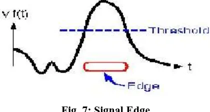
we take the gradient of this signal (which, in one dimension, is just the first derivative with respect to t)

we get the following:

Fig. 7: Signal Edge

Clearly, the gradient has a large peak centered around the edge. By comparing the gradient to a threshold, we

can detect an edge whenever the threshold is exceeded. we can localize it by computing the Laplacian (in one

dimension, the second derivative with respect to t) and finding the zero crossings.

1519 |

P a g e

The above figure shows the laplacian of our one- dimensional signal. As expected, our edge corresponds to a

zero crossing, but we also see other zero crossings which correspond to small ripples in the original signal.

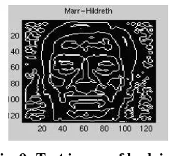
When we apply the laplacian to our test image, we get the following:

Fig. 9: Test image of laplaican

Step 4: Find the zero crossing of the laplacian and compare the local variance at this point to a threshold. If the

threshold is exceeded, declare an edge.

Step 5: Median Filter the image. We apply a median filter because it removes the spot noise while preserving

the edges

Pseudo code for Canny’s Edge detection Algorithm

The Canny Edge Detection Algorithm has the following steps:

 Smooth the image with a Gaussian filter,

 Compute the gradient magnitude and orientation using finite difference approximations for the

partial derivatives,



Apply non-maxima suppression to the gradient magnitude,



Use the double thresholding algorithm to detect and link edges.

Canny edge detector approximates the operator that optimizes the product of signal-to-noise ratio and

localization. It is generally the first derivative of a Gaussian

Smoothing : Let denote the image. The result of convolution of with gives an array of

smoothed data as:

Gradient Calculation: Firstly, the gradient of the smoothed array s[i, j]

is used to produce the x and y

partial derivatives p [t, f] and respectively as:

The x and y partial derivatives are computed with averaging the finite differences over the 2x2 square. From

the standard formulas for rectangular-to-polar conversion, the magnitude and orientation of the gradient can be

computed as:

Here the arctan(x,y) function takes two arguments and generates an angle.

Non-maxima Suppression :Given the being the magnitude image array one can apply the thresholding

operation in the gradient-based method and end up with ridges of edge pixel. But canny has a more

sophisticated approach to the problem. In this approach an edge point is defined to be a point whose strength is

1520 |

P a g e

ridges found by thresholding. This process, which results in one pixel wide ridges, is called “Non-maxima

Suppression”.

After nonmaxima suppression one ends up with an image which is zero

everywhere except the local maxima points. At the local maxima points the value of is preserved.

Thresholding: In spite of the smoothing performed as the first step in edge detection, the non-maxima

suppressed magnitude image will contain many false edge fragments caused by noise and fine

texture. The contrast of the false edge fragments is small.

These false edge fragments in the non-maxima- suppressed gradient magnitude should be reduced. One

typical procedure is to apply a threshold to . All values below the threshold are set to zero.

After the application of threshold to the non-maxima-suppressed magnitude, an array E(i,j) containing the

edges detected in the image is obtained. However; in this method applying the proper threshold

value is difficult and involves trial and error. Because of this difficulty, in the array E(i,j) there may still be

some false edges if the threshold is too low or some edges may be missing if the threshold is too high. A

more effective thresholding scheme uses two thresholds[6,7].

The algorithm performs edge linking as a by-product of thresholding and resolves some of the

problems with choosing a threshold.

Pseudo code for Sobel Edge detection Algorithm



Accept the input image.



Apply mask Sx, Sy to the input image



Apply sobel edge detection algorithm and the gradient



Masks manipulation of Sx, Sy separately on the input image



Results are combined to find the absolute magnitude of the gradient



The absolute magnitude is the output edges



Apply noise smoothing to the original image

Smoothing

:

Filter the image using Sx and Sy to obtain I1 and I2 Estimate the gradient magnitude at each pixel as

S(i,j)=√((I1)2+(I2)2) Marking the pixel as edge points if S(i,j) > β .

Fig. 10: Pixel Edge Point

IV.RESULT ANALYSIS

The merits and the demerits of the different methods is analyzed and summarized.

Type Merit Demerit

Gradient (all 3 Methods) 1. Simple

2. Detection of edges and

their orientations.

1. Sensitive to noise

1521 |

P a g e

Gaussian 1. Using probability for

finding errorate

2. Localization and response

3. Improving signal to noise

ratio.

4. Better detection specially in

noise conditions.

1. Complex Computations

2. False zero crossing

3. Time consuming

Laplacian 1. Finding the place of edges

2. Testing the area around

pixel

1. Malfunctioning at

corners, curves and

where the gray

level intensity

function varies.

2. Not finding the

orientation of edge

because of using

the Laplacian filter

V.CONCLUSION

The following advantages of Sobel edge detector justify its superiority over other edge detection techniques.

(i.) Edge Orientation: The geometry of the operator determines a characteristic direction in which it is most

sensitive to edges. Operators can be optimized to look for horizontal, vertical, or diagonal edges.

(ii). Noise Environment: Edge detection is difficult in noisy images, since both the noise and the edges

contain high-frequency content. Attempts to reduce the noise result in blurred and distorted edges. Operators

used on noisy images are typically larger in scope, so they can average enough data to discount localized noisy

pixels. This results in less accurate localization of the detected edges.

(iii). Edge Structure: Not all edges involve a step change in intensity. Effects such as refraction or poor focus can

result in objects with boundaries defined by a gradual change in intensity. The operator is chosen to be responsive

to such a gradual change in those cases. Newer wavelet- based techniques actually characterize the nature of the

transition for each edge in order to distinguish, for example, edges associated with hair from edges associated

with a face. Detecting edges of an image represents significantly reduction the amount of data and filters out

useless information, while preserving the important structural properties in an image. Hence, edge

detection is a form of knowledge management.

REFERENCES

[1] Canny, John, "A Computational Approach to Edge Detection," IEEE Transactions on Pattern Analysis and Machine Intelligence,Vol. PAMI-8, No. 6, 1986, pp. 679-698.

[2] Lim, Jae S., Two-Dimensional Signal and Image Processing, Englewood Cliffs, NJ, Prentice Hall, 1990,

1522 |

P a g e

[3] Parker, James R., Algorithms for Image Processing and Computer Vision, New York, John Wiley &

Sons, Inc., 1997, pp. 23-29.

[4] Gonzalez, R. C., and Woods, R. E. Digital Image Processing (Reading, MA: Addison-Wesley, 1992

[5] Marr, D., and Hildreth, E. "Theory of Edge Detection," Proceedings of the Royal Society London 207 (1980) 187-217.

[6] Haralick, R. M., and Shapiro, L. G. Computer and Robot Vision, vol.1 (Reading, MA: Addison-Wesley, 1

[7] Jain, |Anil k., Fundamentals of Digital Image Processing, prentice Hall,1989