B ayesian R egression and
D iscrim in ation w ith M any
Variables
by
K ai-M ing Chang
D epartm ent o f Statistical Science
University College London
Thesis subm itted for the degree of D octor o f Philosophy
ProQ uest Number: 10015824
All rights reserved
INFORMATION TO ALL U SE R S
The quality of this reproduction is d ep en d en t upon the quality of the copy subm itted. In the unlikely even t that the author did not sen d a com plete manuscript
and there are m issing p a g e s, th e se will be noted. Also, if material had to be rem oved, a note will indicate the deletion.
uest.
ProQ uest 10015824
Published by ProQ uest LLC(2016). Copyright of the Dissertation is held by the Author. All rights reserved.
This work is protected against unauthorized copying under Title 17, United S ta tes C ode. Microform Edition © ProQ uest LLC.
ProQ uest LLC
789 East E isenhow er Parkway P.O. Box 1346
A bstract
This thesis attem pts to provide general procedures for Bayesian regression and
discriminant analysis with many variables and explore potential problems in the
analysis. For regression analysis, a normal random regression model is assumed,
i.e. the joint distribution of the response variables and the regressors is multivariate
normal given their means and covariance matrix. For the discriminant analysis,
we consider the case th a t each observation is from one of several multivariate
normal populations. In classical statistics, the problem in fitting a multivariate
model with more variables than the number of observations is th a t the estimate of
the covariance m atrix of the m ultivariate normal distribution is singular and the
distribution is degenerate. In Bayesian statistics, this problem can be avoided by
using proper prior assumptions for the covariance m atrix. We assign an inverse-
W ishart distribution (which is a conjugate prior in the case of a non-hierarchical
analysis) for the covariance m atrix and suppose the prior expected covariance
m atrix has a simple structure so th a t the number of hyperparam eters required in
the model is small. Hierarchical modelling of these hyperparam eters is employed.
Although we have managed to keep the model relatively simple with our
strong assumptions, the posterior model is still coiiiplicated. We found ARMS
within Gibbs sampling with multiple chains to be an appropriate MCMC strategy
for fitting our models. Convergence checking for multiple chains MCMC is simple.
Due to the ill-condition of the sample covariance m atrix and the large number of
variables, the computational problems are significant. A ppropriate m atrix manip
ulating and rescaling techniques are required.
Two practical cases are considered as examples, one for regression and the
other for discrimination. Both cases involve NIR spectral data with many vari
ables. The high correlation between variables makes the examples more challeng
much closer to the real situation than the over-simplified one. However, we found
the autoregressive correlation functions do not guarantee better predictions in our
A cknow ledgem ents
Firstly, I would like to thank my supervisour Prof Tom Fearn for his excellent
supervision and patient guidance. The experience of being his student is simply
invaluable. I would also like to express my appreciation to many staff in my
department, especially to Prof A. Philip Dawid and Dr Richard E. Chandler, who
have been so helpful whenever I needed opinions. Special acknowledgements go to
my examiners Prof Paul Garthwaite and Prof Sylvia Richardson for their useful
comments and opinions on my thesis.
I would not forget to thank Dr Suja M. Aboukhamseen and other colleagues
in the research student room for their suggestions, encouragement and friendship.
In particular, I have to thank Ms Anne Andrew for her help to improve my poor
English writing.
My deepest gratitude goes to my parents. Their great love and full support
C on ten ts
List o f Figures 7
List o f Tables 10
N otation 12
0.1 M a tr ic e s ... 12
0.2 Probability ... 12
0.3 M atrix D is tr ib u tio n s ... 13
Chapter 1 Introduction 14 Chapter 2 Bayesian Inference for Linear Regression and Discrim i nation 19 2.1 Bayesian Theory ... 19
2.2 Prior distributions ... 21
2.2.1 Conjugate Prior D is trib u tio n s ... 21
2.2.2 Non-informative Prior D istrib u tio n s... 22
2.3 Hierarchical M o d e llin g ... 24
2.4 Model A ssessm ent... 27
2.4.1 Model C hecking... 27
2.4.2 Sensitivity A n a ly sis... 29
2.5 Bayesian Multivariate Analysis for Normal Variables ... 30
2.5.1 M atrix-variate D is trib u tio n s ... 30
2.5.2 Bayesian Models for a Covariance M a tr ix ... 32
2.5.4 Bayesian D is c rim in a tio n ... 37
Chapter 3 Near Infrared Spectroscopical A nalysis 39 3.1 In tro d u c tio n ... 39
3.2 Theory of NIR A b s o rp tio n ... 41
3.3 Linear Relationship between NIR Spectrum and Concentration of C o n stitu e n ts... 42
3.4 Applications of NIR S p ectro sco p y ... 44
3.5 E x a m p l e s ... 45
3.5.1 Generating S p e c tr a ... 45
3.5.2 Two Examples ... 48
3.6 NIR C a lib ra tio n ... 53
3.6.1 Linear R egression ... 53
3.6.2 Regularised R eg ressio n ... 55
3.7 NIR Discriminant A n a ly sis... 58
3.7.1 Probability A p p ro ach ... 58
3.7.2 Linear and Quadratic Discriminant F u n c t i o n s ... 59
3.7.3 Distance Based M e th o d s ... 59
3.7.4 Estim ation of Mean and Covariance M atrix ... 60
3.8 R e m a r k ... 60
Chapter 4 Markov Chain M onte Carlo 62 4.1 In tro d u c tio n ... 62
4.2 Direct S am p lin g ... 65
4.3 Basic Markov Chain S im u la tio n ... 67
4.3.1 General m e t h o d s ... 67
4.3.2 Full Conditional Distribution and Gibbs S am p lin g ...68
4.4 ARS and ARMS ... 69
4.5 Multiple Sequences MCMC and Convergence A sse ssm e n t... 74
4.5.1 Multiple Sequences MCMC ... 74
4.6 Sampling P l a n ... 78
4.7 Other A pproaches... 80
4.7.1 Improving efficiency ... 80
4.7.2 Convergence A sse ssm e n t... 83
Chapter 5 M odelling a H igh Dim ensional Covariance M atrix 86 5.1 In tro d u c tio n ... 86
5.2 Random F u n c tio n ... 88
5.3 Normal M o d e l... 89
5.4 C o h e re n c e ... 91
5.5 Structural Covariance... 92
5.6 AR(1) and AR(2) Correlation F u n c t i o n s ... 93
5.7 E x a m p le ... 96
5.8 R e m a r k ... 102
Chapter 6 Bayesian Regression w ith M any Variables 113 6.1 In tro d u c tio n ...113
6.2 Sampling M o d e l... 116
6.3 Prior A s s u m p tio n s ...118
6.4 E stim a tio n ... 121
6.5 Some Numerical P r o b le m s ... 124
6.6 E x a m p le ... 126
6.7 Scoring Rule and Sensitivity A n a ly sis...128
6.8 Results and Diagnostics ... 130
6.8.1 Settings for P a ra m e ters... 130
6.8.2 MCMC R e s u l t s ... 131
6.8.3 Model Assessment ... 139
6.9 Modelling with Artificial D a t a ...144
6.9.1 Artificial D a t a ... 144
6.9.2 R e su lts ... 145
Chapter 7 Bayesian D iscrim ination w ith M any Variables 151
7.1 In tro d u c tio n ... 151
7.2 Normal P o p u latio n s... 154
7.2.1 Unequal Covariance matrices ...155
7.2.2 Equal Covariances ... 158
7.3 Hierarchical Normal D iscrim in atio n ... 160
7.3.1 H y p e rp a ra m e te rs... 160
7.3.2 Group Membership P r o b a b il i t y ... 161
7.4 E x a m p le ... 162
7.5 PC A and Logistic Discriminant A n a ly s is ... 164
7.5.1 P C A ...164
7.5.2 Logistic Discriminant A n aly sis...165
7.6 Results and Diagnostics ... 166
7.7 R e m a r k ... 167
Chapter 8 Summary and D iscussion 172 8.1 S u m m a r y ... 172
8.2 Prior In fo rm a tio n ... 173
8.3 Correlation S tru c tu r e ...175
8.4 R eg ressio n ... 176
8.5 D iscrim ination...179
8.6 Model Assessment and MCMC ...179
8.7 C onclusion... 181
Bibliography 183
A ppendix A M atrix D istributions 196
A ppendix B R esults for Regression M odels 198
A ppendix C R esults for Regression M odels for th e Artificial D ata 235
List o f Figures
2.1 One-way normal random effects model when <t^ is given... 25
3.1 Simple diagram of the Tecator Infratec Grain A n a ly z e r ... 46
3.2 Transm itting c e l l ... 46
3.3 Mixed effect of reflection and absorption... 47
3.4 Spectra of 50 wheat s a m p le s ... 49
3.5 Second derivative spectra of 50 wheat s a m p le s ... 50
3.6 Dot plot of the percentage protein in the 50 wheat s a m p le s ... 50
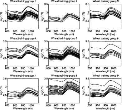
3.7 Transmission spectra of nine wheat varieties in the training set. . . 51
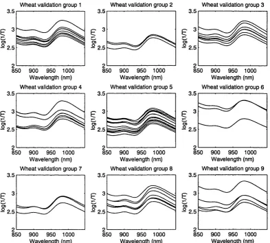
3.8 Transmission spectra of nine wheat varieties in the validation set. . 52
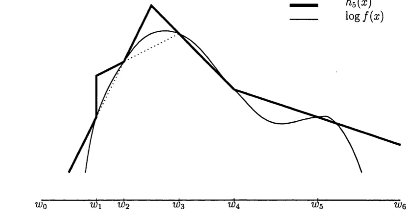
4.1 Adaptive rejection function hs{x) of f { x ) with S5 = {iüq, • • •, lUg} . 71 4.2 Adaptive rejection function h6{x) of f { x ) in figure 4.1, where 1x3 is the rejected value in step 3 of ARMS... 72
4.3 The contour and a sampling path of Gibbs sampling for a bimodal bivariate distribution with well-separated peaks... 75
4.4 Adding a new p e a k ... 82
5.1 Sample standard deviation (S.D.) the NIR spectra in the first ex ample in chapter 3 . 4 . 2 98
5.2 Sample standard deviation and a multiple of |sample mean|°'^ of the 2"^ derivative spectra in the first example in chapter 3 .5 .2 ... 99
5.4 The 2"^ derivative spectra, their covariance matrices and correlation
m atrices... 110
6.1 Graphical presentation of the non-conjugate random regression model 120 6.2 Scatter plots of MCMC samples of 9, Ar,T) and F ... 135
6.3 Rao-Blackwellised estimates of regression coefficients ... 136
6.4 Estim ated standard deviations of the posterior /3 ... 138
6.5 Model Diagnostics for M.a, M.b and M . c ...140
6.6 T - a , t- 6 and B - a relationships given r ... 142
6.7 50 centred artificial s p e c tra ...143
6.8 Dot plot of the 50 artificial data for Y ...143
6.9 Sample Y against residual for the real data in and the artificial data using the given p... 144
6.10 Original j3 and the Rao-Blackwellised estimates of / ? ... 148
B .l MCMC output of regression model M.a (4 chains plotted together) 202 B.2 MCMC output of regression model M.b (4 chains plotted together) 206 B.3 MCMC output of regression model M.c (4 chains plotted together) . 210 B.4 MCMC output of regression model M.d (4 chains plotted together) 214 B.5 MCMC output of regression model M.e (4 chains plotted together) . 217 B.6 Histograms of MCMC samples for the param eters in regression model M . a ...221
B.7 Histograms of MCMC samples for the param eters in regressi model M .b ... B.8 Histograms of MCMC samples for the param eters in regressi model M . c ... B.9 Histograms of MCMC samples for the param eters in regressi model M .d ... B.IO Histograms of MCMC samples for the param eters in regression model M . e ...232
on
. 224 on
. 227 on
C .l Histograms of MCMC samples for the param eters in regression
model M . a ...236
C.2 Histograms of MCMC samples for the param eters in regression model M .b ...239
C.3 Histograms of MCMC samples for the param eters in regression model M . c ... 242
D .l MCMC output of discriminant analysis M . a ... 247
D.2 MCMC output of discriminant analysis M . b ... 248
D.3 MCMC output of discriminant analysis M . c ... 249
D.4 Histograms of samples for the parameters in discriminant analysis M .a ... 250
D.5 Histograms of samples for the parameters in discriminant analysis M.b ... 251
D.6 Histograms of samples for the parameters in discriminant analysis M .c ... 252
E .l Xt^Xt for the original s p e c t r a ...254
E.2 MCMC estimate of the mean marginal (1 + 0)Qxx for M . a ... 255
E.3 MCMC estimate of the mean marginal (1 + 6)Qxx for M . b ... 256
E.4 MCMC estimate of the mean marginal (1 + 0)Qxx for M.c ... 257
E.5 X i X i for the 2"^ derivative s p e c t r a ... 258
E.6 MCMC estimate of the mean marginal (1 + 9)Qxx for M . d 259 E.7 MCMC estimate of the mean marginal (1 4- 9)Qxx for M.e ... 260
E.8 Xt^Yt of the original spectra and MCMC estimates of the mean marginal (1 + 9)Qxt, of M.a, M.b and M .c ...261
List o f Tables
3.1 W heat data: numbers of samples of each v a r ie ty ...48
5.1 Five combinations of d ata and structural correlation m atrix . . . . 97
5.2 Prior settings for the example in section 5 . 7 ... 100
6.1 Param eters in the five m o d e l s ... 129
6.2 MCMC sample means and s.d. (in parentheses) of parameters . . . 132
6.3 MSEP of a PCR model and three Bayesian models for the origi
nal spectra and a PCR and two Bayesian models for the second
derivative spectra... 134
6.4 M.b with fixed r ...141
6.5 M.e with fixed <j>i...141 6.6 MCMC sample means and s.d. (in parentheses) of parameters for
the artificial s a m p l e s ...147
6.7 MSEP of the models for the artificial d a ta ...148
7.1 Param eters in M.a, M.b, and M.c for discrimination analysis . . . . 162
7.2 MCMC estimates of parameters and their standard deviations (in
p are n th e se s)...169
7.3 Number of correct classifications (C.C.) on 58 validation samples . . 169
7.4 Number of correct classifications (C.C.) on 234 training samples . . 169
7.5 Frequency tables of the G M P’s ...170
N o ta tio n
0.1
M atrices
I: Identity matrix.
Ip\ a p by p identity matrix. L e t X b e a n a r b i tr a r y m a trix :
X^\ the transpose of m atrix X .
Xpxq: an alternative notation for X in which p x q indicates the dimension of X .
S u p p o se X is a s q u a re m a trix :
X > 0: X is positive definite.
X > 0: X is positive semi-definite.
trX : the trace of X .
|X |: the determ inant of X.
X~^: the inverse m atrix of X .
0.2
Probability
I : conditional on or given.
E{X): Expectation of X .
C{X): Covariance m atrix of a column vector X , C{X) = E ( X X ^ ) — E { X ) E { X y P{D): probability measure of event D.
p{X): probability density or mass function of random variable X .
0.3
M atrix D istributions
J\f: m atrix normal distribution. W; W ishart distribution.
XW: inverse-Wishart distribution.
T: m atrix-t distribution.
C hapter 1
Introduction
This thesis deals with regression and discriminant analysis with many variables
in a Bayesian framework. Regression and discriminant analysis are im portant
multivariate statistical techniques th a t have been widely applied in many fields.
In regression analysis, one attem pts to relate two sets of variables with a model
so th at one set of the variables can be predicted by the other set. In discriminant
analysis, one aims to predict which of two or more groups an object belongs to
using a model th a t has as its input a set of variables we observe for the object.
If we take the group membership of an object as a categorical variable, we can
link the discriminant model to the regression one. Problems arise in fitting models
and making predictions when there are many more variables than the number of
observations we use to fit the model. Two major problems are the singularity of
sample* covariance matrices and overfitting, which are also two general problems
in statistics.
The topic of the thesis is motivated by the analysis of near infrared (NIR)
transmission spectroscopy, where chemical analysts take the (possibly transformed)
NIR absorbances of a sample , e.g. a chemical compound, at certain wavelengths
as predictor variables and use these measurements to predict chemical composition
of the sample or to classify the sample to one of several groups. Often, the number
of wavelengths observed can be up to one thousand or even more. T hat is, for each
sample there can be more than one thousand predictor variables observed. The
linear model has been widely accepted in analysing d ata from NIR spectroscopy.
According to the Beer-Lambert law (see chapter 3), an NIR transmission spectrum
of a sample is, under ideal conditions, a linear combination of the NIR transmission
spectra of the constituents of the sample, and the weight of each linear component
would be proportional to the concentration of the corresponding constituent in a
sample. The ideal conditions rarely hold in practice, but linear models have been
found to work well in most applications. NIR transmission spectra arise from the
absorption of light by organic chemical bonds. A chemical bond has absorption
peaks at certain wavelengths, which depend on the atoms at the two ends of the
bond and on their relationship with other atoms in the molecule. An individual
absorption peak has a smooth bell shape. Unfortunately a typical NIR spectrum
will contain many thousands of overlapping peaks, and the chemical information
we wish to extract will occur in several (not precisely predictable) places and be
seriously mixed up with other information. Thus, the simple approach of select
ing a small number of relevant wavelengths is not usually appropriate, and it is
common to use models where all the spectral variables are taken as predictors.
Standard statistical inferences for regression and discriminant analysis use
least squares estimation (LS) or maximum likelihood estim ation (MLE) to esti
mate the parameters in the models. However, in the cases when we are using more
variables than samples and the variables cannot be pre-selected in order to reduce
the number of variables so th a t they are less than the number of samples, LS esti
mation and MLE of parameters are inappropriate because they require inversion of
the sample covariance matrix, which is a singular m atrix. Many regularised m eth
ods aimed at keeping as much information from the predictor variables as possible
whilst avoiding the inversion of a singular m atrix have been developed. Existing
methods for regression analysis include principal components regression (PCR),
partial least squares regression (PLSR), ridge regression (RR), and continuum re
analysis (PCA) to overcome the problem of singularity of the sample covariance
matrix. One can refer to Brown [23], Martens and Næs [94] and Osborne, Fearn,
and Kindle [100] for further details of these methods as well as their application
in NIR analysis.
When using more variables than observations in a model, there is always
a risk of overfitting. In the regression case when we have more variables than
observations, we can always (unless collinearity means th a t the variables lie in a
subspace of dimension less than the number of observations) find a set of coef
ficients which fits the data perfectly. In general, when the number of regressors
increases, the model always fits the data better. However, the variance of predic
tion is not always reduced when the number of regressors goes up (Seber [113]).
Models th a t fit data too well usually predict future observations badly. One way
to check the models is to use the cross-validation method (Stone [118]), which has
been widely employed in many applications. The purpose of cross-validation is to
make sure a fitted model can reasonably predict or classify future observations by
fitting the model with a training data set and assessing the performance of the
fitted chosen model on validation data with an appropriate scoring rule. We use
it as a method to assess our models.
This thesis explores the properties of normal regression and discrimination
with many variables in a Bayesian framework. The Bayesian approach makes infer
ence by combining prior knowledge of the model with observed data. The inference
on the unknown quantities of interest is summarised by a posterior distribution
derived using Bayes’ rule. Statistical methodology in a Bayesian framework has
developed considerably since the 1960’s, not only because it provides an easily
understood way of summarising results, but also due to progress in computer
technology and developments in Markov chain Monte Carlo simulation (see Gilks
et al. [73]). Because of these advantages, the Bayesian approach is able to deal with very complex models, which may involve many param eters with complicated
relationships between them. It is also known th a t the Bayesian approach does
sam-pies. The insufficient rank of the d ata is made up by the use of prior information.
Therefore, it is natural to consider the Bayesian approach for modelling with many
variables.
It is well known th at prior assumptions become im portant when there are
more variables than observations. A major focus in this thesis is the effect of prior
assumptions about the covariance m atrix of the predictor variables. Since there are
many variables, the covariance m atrix is huge. In order to reduce the number of
parameters and make the modelling process tractable, we assume there is a simple
structure in the covariance matrix, which requires only a few param eters to de
scribe, chosen so th at an analytical inverse m atrix and determ inant are available
for computational efficiency. At the same time we try to use realistic prior as
sumptions, i.e. ones th at would generate data resembling those we have observed.
The structure of the expected covariance m atrix should satisfy the principle of
structural coherence defined by Brown [23], th at the structure of the expected
covariance m atrix of a refinement of a random vector should be generated by the
same structural consideration th at generates the expected covariance m atrix of the
random vector. A prior distribution is assigned to the param eters in the expected
covariance m atrix so our models are hierarchical.
For regression analysis, we consider the non-conjugate m ultivariate normal
random regression model which has been conceptually suggested by Makelainen
and Brown [93]. The non-conjugate model was proposed in order to avoid the de
terministic property of the natural conjugate regression model. Dawid [43] proved
th at under the normal-inverse-Wishart prior assumption, the natural conjugate
regression model with an infinite number of predictor variables can predict the
future precisely when the parameters in prior distributions are known. The prop
erty is called determinism by Dawid. Other applications of Bayesian regression
with many variables either consider information compression (e.g. West [126]) or
focus on variable selection with a computationally convenient prior assumption
to improvement in predictive performance.
For discriminant analysis, we assume a m ultivariate normal distribution
within groups and apply Bayes’ formula to obtain the posterior group membership
probability of an object. Our main focus is on the use of more realistic prior
distributions for the variance parameters of a full model with many variables.
Posterior predictive probabilities of a sample belonging to different groups are
calculated and taken as a criterion for allocating the sample. Recent applications
in discrimination for NIR data can be found in Brown et al. [24] and Fearn et al. [56].
We use two examples of NIR spectroscopic d ata of wheat samples, one for
regression and one for discrimination. In both examples, measurements of the NIR
spectrum of each wheat sample are recorded digitally at a hundred equally spaced
wavelengths. In the regression example, there are 50 samples in total, while there
are in total 292 samples of 9 varieties (groups) for the discrimination problem.
Bayesian theory and stochastic simulation provide the possibility of han
dling complicated situations and producing easily understandable summaries of
the inference results. Although in our examples the predictor variables are very
highly correlated, the model we investigate in this thesis would be applicable to
situations with less strongly correlated variables. Moreover, the MCMC simula
tion scheme (ARMS within Gibbs sampling) we employed for fitting our models
is a very general method which is very useful in fitting models with many param
eters. In practice, d ata analysts are facing ever more situations where there are
many variables in their models. Examples exist in the fields of molecular biology,
econometrics, geostatistics, chemometrics, etc. For instance, genetic data analysis
C hapter 2
B ayesian Inference for Linear
R egression and D iscrim in ation
2.1
Bayesian Theory
The idea of Bayesian inference first appeared in Thomas Bayes’ paper in 1763 [6],
where he proposed a uniform distribution for the param eter in the binomial dis
tribution. Later, Laplace independently discovered the general form of Bayes’
theorem. The idea of Bayes was then largely ignored for two hundred years. Dur
ing the second half of the 20th century, scientists started to realise the potential
of Bayesian methodology and applied Bayes’ theory in many areas.
Bayesian inference for an unknown quantity yields a probability distribu
tion, which is derived by combining the observed d ata with a probability model
for the quantities we observe and the unknown quantities about which we want to
learn. Bayesian theory is based on a simple and fundam ental probability rule
m « i « ) - £ 2 ^ , (2.1)
represents the prior probability of the hypothesis, while P{D) is the marginal prob ability of the d ata over all possible hypotheses. Therefore, in Bayesian modelling,
we need a sampling distribution which the d a ta we observe are assumed to follow, and a prior distribution of all possible hypotheses, which formalises our prior be lief about the hypotheses. Rule (2.1) provides the distribution of the hypothesis
conditional on the data we observe, which is called the posterior distribution of the hypothesis. The subject of a hypothesis can be parameters, predictors, or even a
model.
For example, suppose X is a continuous random variable from sample space
%. Its density function is p{X\6), where 6 is from a continuous param eter space 0 , and p{6) is the prior density function of 9. We observe Xi^X2,. . . , for X as train
ing samples to fit (train) our model. The observations are sampled independently
with the same density function as X , hence.
p { x i , X 2 , . . . , X n \ 0 )
= J][p(a;i|0).
i=lWe can then derive the posterior density function of 9,which is
= (2.2)
p [ X i , X2, . . . , X n )
where
p { x i , X2, . ^ . , X n ) = J ^ p { x i , X2, ... , X n \9) p {9) d9 = j ' ^ p { x i \9) p [9) d9.
Now, if we want to predict future m observations of X , we use the predictive density function of X based on the posterior distribution of 9. Suppose we want
to predict • • •, ^n+m, which are conditionally independent given 9. The
posterior predictive density function is
P {^n + li ^ n + 2 j ' • • Î ^ n + m 1 ^ 1 j ^ 2 > • • • j ^ n )
= I p ( ^ X j i ^ i j Xj i ^ 2 ^ • • • j ^ n + m \ 9 ^ p { 9 \ x \ ^ X 2 i • • • j X j i ) d 9
Je
« m
= J Y { p { X n + i \ 9 ) p { 9 \ x i , X 2 , . . . , X n ) d 9 .
Equation (2.1) is called Bayes’ formula or Bayes’ rule. W ith Bayes’ formula,
we update the prior model th at is based on our prior knowledge to a posterior
model th at is conditional on the evidence we observe.
For a more detailed introduction to Bayesian statistics readers may refer
to [12], [65], or other Bayesian textbooks. In this chapter, we introduce concepts
th at are im portant in Bayesian regression and discriminant modelling with many
variables.
2.2
Prior distributions
The prior distribution plays an im portant role in Bayesian inference. It introduces
the expert’s knowledge of the unobservable param eters in a model by formalising
the expert’s opinion about the parameters as prior distributions. However, speci
fying a prior distribution is not an easy step. The choice of prior distribution for
the parameters is probably the most controversial issue in Bayesian statistics.
2.2.1 C onjugate Prior D istrib u tions
In Bayesian statistics, when the joint prior distribution and the joint posterior dis
tribution of parameters in the sampling distribution belong to the same parametric
distribution family, the prior distribution is called a conjugate prior distribution
for the sampling distribution, and Bayesian analysis with a conjugate prior is called
conjugate analysis.
Consider again the example in the previous section. After the model has
been set up, the most complicated part of the inference is the integration required
to calculate the denominator in (2.2). Since the denominator in (2.2) is a constant,
we have
p { 0 \ x i , X 2 , . . . , X n ) c C p { X i , X 2 , • • • , X n \ 0 ) p { 9 ) .
If a posterior distribution belongs to some known param etric distribution fam
ily, the integration is actually unnecessary, and the distribution can be identified
The advantage of using a conjugate prior distribution is not only th at in
tegration can be avoided. Since the prior distribution and posterior distribution
belong to the same param etric distribution family, the inferential process is just a
m atter of updating the parameters in the prior distribution so the cost of comput
ing is greatly reduced. The disadvantage is th a t the choice of prior distribution
for a given sampling distribution is very limited, and available conjugate prior
distributions may not be adequate to represent our prior opinion. Modelling with
non-conjugate prior distributions th at are more realistic is in many cases unavoid
able. Even so, conjugate analysis has been applied in many practical cases due to
the convenience in computing. Examples of conjugate analysis can be found in all
Bayesian textbooks.
2.2.2
N on-inform ative Prior D istrib u tion s
It is often the case th at the prior information for a param eter in a model is very
limited or uncertain. In this case, one would naturally expect to assign a prior
distribution th a t makes little contribution to the posterior distribution of the pa
rameter and ‘let the data speak for themselves’, i.e. let the data dominate the
posterior distribution of the parameter. Non-informative priors (also called vague
priors) have been frequently used in Bayesian applications in order to represent
prior ignorance.
The simplest type of prior th at may represent prior ignorance is Laplace’s
rule, or the principle of insufficient reason (see Kass and Wasserman [86]). It
assumes every value for the param eter is equally possible, i.e.
p{9) DC c .
Such a prior was first applied by Bayes and Laplace. W hen the param eter space is
bounded, p{6) is a uniform distribution. When the param eter space is not bounded,
p{9) is not a well-defined distribution because its integral over the param eter space is infinite. One problem with using this fiat prior is th a t it is inconsistent under
density function of 9. Let ÿ be a re-param eterisation of 9 with (j) = exp(0). The prior density function of ^ is a multiple oil/(f), which does not follow Laplace’s rule of prior ignorance. Jeffreys [82] proposed a procedure for creating prior density
functions which are invariant to re-parameterisation in ways th at will be described
below. The Jeffreys’ prior p{9) for the param eter ^ in a probability model is given by
p { 6 ) (X y # ,
where I{9) is the Fisher information m atrix of 9, The Jeffreys’ prior has been widely used in one dimensional cases. However, its performance in higher dimen
sional cases is not always satisfactory.
Invariance has been considered to be im portant in creating non-informative
prior density functions. Dawid [42] concludes th a t there are three types of invari
ance:
• Param eter invariance: The prior distributions of two models derived under
this principle should be equivalent when one model is a re-parameterised
version of the other.
• D ata invariance: Suppose T is a transform ation of X and th a t Y and X
have a common parameter 9. The prior distributions of 9 derived from the distributions of Y and X under this principle should be the same.
• Context invariance: No features of the structure, meaning, or context of
a model other than its distribution model should be taken into account in
forming an invariant prior.
Jeffreys’ prior is an example th at satisfies these three principles. O ther variations
of these principles exist. Dawid [42] and Kass and Wasserman [86] give further
coverage of invariance theory.
Alternatives to Jeffreys’ prior are available. Some of them are based on min
imising the information in the prior distribution. Berger and Bernardo (see [9, 10,
distance between the posterior density and the prior density. This produces in
variant non-informative priors. Many authors have investigated maximum entropy
priors. Jaynes proposed a maximum entropy method th at also produces invariant
priors. There are many other methods in the literature th a t can be used to pro
duce non-informative priors. Kass and Wasserman [86] provide a review of formal
rules for selecting non-informative prior distributions.
Although there are many methods for creating non-informative priors, most
of these priors have improper density functions. There are many problems in
using improper priors, especially in modelling with many variables. The major
problem is th a t improper prior density functions are very likely to yield improper
posteriors. The use of improper priors is widely accepted if the resulting posterior
density functions are proper. W hether a posterior is proper or not can usually be
easily examined if the model is simple. However, it is no longer easy when the
model is more complicated. Kass and Wasserman [86] also summarised four other
problems: incoherence and strong inconsistencies (see the examples in Stone [119]),
the dominating effect of the prior, inadmissibility, and marginalisation paradoxes
(see Dawid, Stone and Zidek [46]).
2.3
Hierarchical M odelling
In many applications, there may be more than one param eter in the sampling
distributions. Frequently, these parameters are related to each other by some
hierarchical structure according to the nature of the application. Suppose we have
random quantities A , Oi and 6 2 whose joint density function is p(%, ^1, %). The hierarchical structure of these random quantities is based on a prior relationship
th at X is independent of 6 2 given 6\, which is denoted by
XAL6 2\ei
by Dawid [40]. The relationship of X , Oi, and 6 2 can also be illustrated in a simple
directed graph
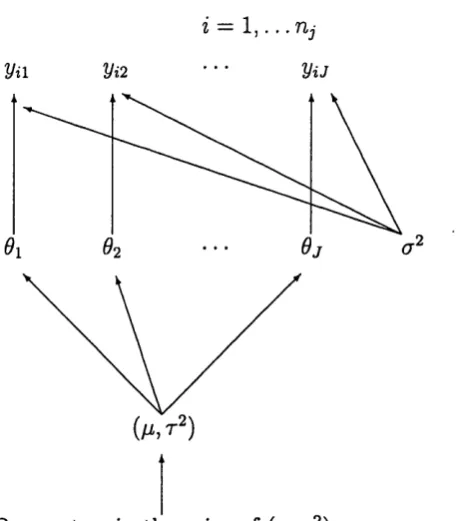
Z — 1 j . . . TZj
yn Vi2 Vi J
.2
ÔJ a
Parameters in the prior of (/i, r^)
Figure 2.1: One-way normal random effects model when is given.
which shows the hierarchy. The conditional distribution of X depends only on the param eter connected to it in the graph, which is 6i in this case, and hence, the
joint distribution can be expressed as p { X\6i)p{di\6 2)p{0 2). A param eter which
does not connect to X is called a hyperparameter, whose prior distribution is called a hyper prior distribution.
Consider the one-way normal random effects model as a simple example.
Suppose there are J independent experiments. In the experiment, there are
rij d ata points, with unknown mean 6j and common known variance cr^ for each
observation. Denote the observation in the experiment as pij. Therefore,
VijlOj ~ N {6j, cr^)
independently for i = 1 , . . . , rij and j = 1 , . . . , J . The conjugate prior distribution
of 6j is N { p , t ‘^) for every j , and 6j are independent of each other given hyper
parameters p, and r^. The hyperparameters are given prior distributions. The hierarchical structure of the model is presented in the figure 2.1.
9J. If the joint distribution of these param eters is invariant to permutations of the indices ( 1 , . . . , J), we say 0 i , . . . , are exchangeable. In practice, such
an assumption is frequently made because there is not enough information to
distinguish one param eter from the others. The most simple assumption is th at
the parameters 9 i , . . . , 9 j are mutually independent with identical prior density functions conditional on some hyperparameters (de F inetti [47]). The one-way
normal random effects model is one example. The param eters OjS are exchangeable given // and and the observations {yij,y2j, •. -ynp) are exchangeable given 6j.
The observations are referred as partially exchangeable because they are only
exchangeable in the subset to which they belong. Exchangeable observations are
often referred to as iid samples given a set of param eters.
In many applications, the graph for the random variables and parameters in
a model is quite complicated. Models with a hierarchical configuration can usually
be displayed systematically even though the number of param eters is large. The
joint distribution of random variables and param eters can always be factorised
as the product of some conditional prior density functions with some parameters.
Statistical inference with the resulting factorised joint distribution is often more
computationally efficient (see examples in the next paragraph). However, the
hierarchical structure of a model should follow the structure of the application
itself.
Hierarchical structure has been exploited in many statistical models, e.g. in
the linear model of Lindley and Smith [91], for discrimination in Brown et al [24], in the spatio-temporal model in Zhu and Carlin [132], for experimental design
in Tiao and Box [123], longitudinal analysis in Kass and Steffey [85], categorical
d ata in Albert and Chib [1], and many other examples. Due to the progress
in computing ability, hierarchical modelling has been applied in more and more
practical cases. For example, Johnson [83] proposed a hierarchical specification for
image analysis; Cohen et al. [34] considered criminal cases relating to drugs and robbery with a hierarchical model; a DNA profile modelling application can be
Besag and Higdon [15] used it in agricultural experiments. There are also many
applications in medical statistics, such as Congdon and Best [35]. Most of the
applications have to employ MCMC techniques because of their high-dimensional
parameter space and complicated posterior structure.
2.4
M odel A ssessm ent
A fundamental problem in modelling is th a t we can rarely claim we know the true
model for the events we observe. Ideally, we would like to explore all possible
models in the universe in order to find the best one. However, it is impossible
to fit universal models. Instead, we choose the best model among a collection of
models, or we gradually modify our original model until we accept one.
Research in model assessment has an extensive literature. Relevant topics
include model comparison, outlier detection, sensitivity analysis and others. In
this section we briefly review some of these topics. We divide the topics into three
categories: model checking, model selection and sensitivity analysis. Model check
ing concerns whether our model describes or fails to describe the data. Examples
are outlier detection, influential observation detection, checking of model assump
tions and overall fitting. Model selection means to select the best model from a
collection of models or to select the best subset of variables in a model. Sensitivity
analysis focuses on the stability of the models we choose. Many of these methods
for model assessment are simulation-based. In this section, we briefly introduce
some topics in model checking and sensitivity analysis.
2.4.1 M od el Checking
In classical analysis, residuals have been an im portant source of information for
model diagnostics. One can simply plot the residuals to check whether there
are outliers or whether the model assumption is right. A similar idea has been
brought into Bayesian analysis. In classical statistics, the residual is defined as the
the fitted model, and each residual is a fixed value because the fitted value is
a fixed value. However, the residuals in Bayesian statistics are not fixed values
but have a distribution, since the prediction of a future value is summarised by
a posterior predictive distribution. Box [16] and Rubin [1 1 1] considered more
general residual functions for examining model adequacy in a Bayesian context.
The development of model checking is generally based on the posterior predictive
distribution of samples. Simulation is frequently required because the posterior
predictive distributions are usually non-standard.
One method of checking the appropriatness of a model is proposed by Gel-
man et ai [6 6]. This method is based on the method developed by Rubin [1 1 1]. A proper discrepancy variable T (a function of data) is defined for a model. Let (notation of Gelman et al.) represent the d ata generated by the posterior pre dictive distribution and represent the observed data. The posterior predictive
p-value p(T(y'‘®P) > is calculated to evaluate the model. Many exam
ples are shown in Gelman et al. [65]. Also see Gelman and Meng in Gilks et o/.[73]. Gelman et al. [6 6] also emphasise the importance of using a graphical comparison of the histogram of y°^^ and the histogram of y^^^. The graphical display of these histograms usually provides more information than a p-value can provide. One
problem with Gelman et al. [6 6]’s method is th at have been used to fit the model which produces As a result, their method is less critical of the model
than it might be (see Dey et al. [50]). It cannot prevent overfitting.
Some authors focus on the model diagnostic methods for hierarchical mod
elling. Albert and Chib [1] consider outliers, exchangeability and other properties
for conditionally independent hierarchical models. Their approach is in fact a
model comparison approach. Dey et al. [50] propose a stage-wise checking method to examine the failure in each stage of the structural assumption for the hierar
chical models. Their method is also based on the discrepancy measurement as
in Gelman et a/. [6 6]. Hodges [80] considers the general hierarchical linear m od els and suggests tools for examining candidate added variables, transformations,
Outlier detection is also a topic considered. One example was given by
Chaloner and Brant [31], who propose an outlier detection method for Bayesian
linear regression when the variance of the random errors is known. The probability
of an observation being an outlier is calculated. A graphical diagnostic tool is also
proposed. A similar idea is to check whether there is any observation th at is
very influential to the model. For a review see P ettit [101]). Hodges [80] also
considered using some graphical tools in his paper. Some authors suggest the
use of cross-validation so th at the replicated d ata generated from the posterior
predictive distribution are compared with observations th a t have not been used to
fit the model. Examples of model checking using cross-validation are P ettit and
Young [102] and Gelfand et ai [62]. Dey et al. [50] and Gelman et al. [65] provide reviews of many methods for model checking.
2.4.2
S en sitivity A nalysis
A good model does not only fit the d ata well. We also expect the model to be
robust. In a robust Bayesian analysis, small changes in a prior model (the sam
pling distribution and the prior density functions for the param eters in the model)
should not cause significant changes in the posterior model (posterior distributions
for parameters and the posterior predictive distribution) . The main purpose of
sensitivity analysis is to evaluate the stability of the models.
Bayesian sensitivity analysis examines the mapping from prior to posterior
across a class of sampling models or prior distributions (see Draper [52]). To test
priors only, one fixes the sampling distribution and varies the prior distribution.
Usually, the prior distribution is varied by changing the values of the parameters
of the prior distribution. In such a case, one selects several param eter settings
in the same distribution family as priors and obtains the corresponding posterior
distributions or predictive distributions, then compares the posterior means of
parameters of models or compares the predictive performance using a suitable
scoring rule, for example by cross-validation in D raper [53]. Berger [8] suggests
e-contamination class is defined as
r = {tt : 'k{9) = (1 - e)'Ko{0) + eç(^), ç G £},
where 7To(0) is a chosen prior of 0 < e < 1 is the weight of q{9) and £ is a class of possible “contaminations.” A different approach is to consider the Bayes
risk of candidate models with different prior settings (see Berger [8]). Kass and
Raftery [84] suggested using sensitivity to examine whether the Bayes factor is
sensitive to the prior or not. A theoretical introduction to Bayesian posterior
and risk sensitivity analysis is available in Berger [8]. Alternative approaches are
suggested in Weiss [125].
When the posterior model can be obtained analytically, sensitivity analy
sis can be easily achieved since the posterior means of param eters or the scores
of predictive performance are simply functions of given parameters and observed
quantities. When the analytical posterior model is not available, sensitivity analy
sis is time-consuming. The same process of numerical approximation or stochastic
simulation of parameters has to be done for each prior setting. There seems to
be no short cut for doing sensitivity analysis when a model is complicated. When
there are many parameters, the amount of computing for sensitivity analysis con
sidering variation for every param eter is tremendous.
2.5
Bayesian M ultivariate A nalysis for N orm al
Variables
2,5.1 M atrix-variate D istrib u tions
In this subsection we briefly introduce m atrix-variate distributions, including ma
trix normal, W ishart, inverse-Wishart, matrix-T, and m atrix-F distributions, which
are involved in the models in this thesis. We follow the notation for these distri
butions developed by Dawid [41]. The notation is not necessarily the same as
the notation for these distributions which has been considered by the other au
for matrix-variate conjugate analysis can easily be carried out. The density func
tions of these distributions are provided in appendix A.
M atrix Normal
The distribution of an n by p random m atrix X with independent standard normal elements is denoted hy X ^ For constant matrices A with n columns,
B with p rows, and M with the same dimension as A X E , the distribution of
M -I- A X E is denoted by M -f W(A, E), where AA^ = A and E^E = E. W ishart D istribution
Let Xnxp ~ Epxp), and Z = X ^ X . The distribution of Z is a W ishart distribution with shape param eter n and scale m atrix Epxp, denoted as W (n; Epxp). For a general W ishart distribution, the shape param eter can be any positive real
number, and the scale m atrix needs to be non-negative definite. Suppose ^ ~
W(i/; A), the expectation of 'ijj is i/A. Inver se-W ishart D istribution
Let a p by p m atrix 0 be inverse-Wishart distributed with shape param eter 6 > 0
and scale m atrix E > 0, we denote it as $ ^ X W (5;E). The expectation of 0
is T,/(ô — 2) ÏÏ Ô > 2 and E > 0. The distribution of 0"^ is a W(i^;E~^), where
ly = Ô + p — 1.
M atrix-t D istribution
M atrix-F distribution
The p x p random m atrix U having a matrix-variate F distribution with parameters
u, 6, and K is denoted as C/ ~ ^(i^, 5] K), with mean i / K / {6 — 2). Suppose U \ ^ ~ W(z/; <E>) with 0 ~ TW{5\ K), then marginally U ~ 5\ K). l i U ^ T{i>, 6] Ip),
then U~^ ~ J^{0 p — l , u — p V, Ip). If T ~ T { 6 ’, Ip, Iq) then T*T ~ !F{p, J; Iq).
2.5.2
B ayesian M odels for a Covariance M atrix
In multivariate analysis, we often assume variables are normally distributed. For
a multivariate normal distribution, there are two parameters: the mean and the
covariance matrix. A covariance m atrix is also called a variance m atrix, a disper
sion matrix, or a variance-covariance matrix. Often, the mean and the covariance
m atrix are unknown, and we have to assign prior distributions for them. Sup
pose we assume the mean is again from a m ultivariate normal distribution, then
there is another covariance m atrix to be specified. Therefore, the assumption for
covariance is inevitably an im portant issue.
Sometimes, we may have reliable information about the covariance m atrix,
but frequently we do not have much information about it, and diffuse distributions
such as inverse-Wishart with small shape param eter or a flat prior to represent
our prior ignorance are frequently in use. Suppose p is the number of variables in our model. For small p with many data, the assumption for the covariance m atrix is usually not im portant because data speak for themselves and the estimation
is usually very close to the maximum likelihood solution. However, the prior
distribution is increasingly informative when the number of variables increases.
Therefore, more consideration has to be given to the prior assumptions. In this
section, we introduce some of the frequently used prior assumptions for covariance
matrices.
Jeffreys’ prior where p(E) oc and a flat prior p(E) oc 1 are both
commonly used as non-informative prior for the covariance m atrix E. However,
care must be taken when applying them because both of them may lead to improper
a small data set. There are also other alternatives. For example, Daniels [37]
derived a non-informative prior for the covariance m atrix as a hyper param eter in
a hierarchical model.
A conjugate prior is always an attractive assumption because of the con
venience in manipulation. The natural conjugate prior for covariance matrices of
normal variables is the inverse-Wishart distribution. Chen [32] for example as
sumed the natural conjugate prior, which is inverse-Wishart for the covariance
m atrix and assumed the parameters in the inverse-Wishart known. However, it
is known th at the inverse-Wishart prior lacks flexibility. Once its mean has been
decided, we can only use the scalar shape param eter to determine the distribution
of the p X ( p H -1)/2 parameters in the covariance matrix.
Suppose a p by p m atrix S ~ XW{5\ 0 ) ,where 0 > 0. Let C7ÿ be the ij th element of E and (f)ij be the ij th element of 0 . According to Theorem 5.2.2 in Press [103],
var(crjj) =
(5 - 2)2(<5 - 4)
for 5 > 4,
var(m;) = ^
( 5 - l ) ( ( 5 - 2 ) ( 5 - 4 ) ’
for ^ > 4 and i ^ j , and
= ( 5 - 1 ) ( 5 - 2 ) ( 5 - 4 ) ’
for 5 > 4 (for all When the shape param eter is small, the variance is
large. When ô < 4, the variance does not even exist. Therefore, an inverse-Wishart distribution with a small shape param eter is usually considered as a diffuse prior,
while for one with large ô, the prior is more informative.
Consider the conjugate model for a 1 by p random vector X
X ~ J\A(1,E), S ~
for E is ZW{5 4- n; x^x + 0 ), with expectation {x^x + ^ ) / {5 + n — 2). When the number of samples n is very large, E{T,\x) is almost x ^ x / {ô-\-n — 2) given the same 0. When n is small, 0 is more influential for the posterior E.
In a non-hierarchical model, ô and # are considered as known constants although one may not be so certain about how well the inverse-Wishart distribution
represents our prior belief. Further assuming a hyper prior distribution for the
hyperparameters extends the flexibility of the prior conflguration. Moreover, the
marginal distribution of E can be more diffusive in a hierarchical model. Therefore,
the hierarchical model can be less sensitive than a non-hierarchical one.
An inverse-Wishart distribution with a structured scale m atrix has been
considered as the prior for E by many authors. Such an assumption reduces the
number of parameters fro m p (p + l) / 2 to a small number so th a t the computational
aspect of model inference is simpler. Ideally, the structure should be consistent
with our belief in the data. However, the real structure of a covariance m atrix is
usually too complicated or simply unknown, especially in a high dimensional case.
The most common and simple form is the diagonal m atrix with equal diagonal
elements. Dickey, Lindley and Press [51] consider an intraclass covariance structure
for the scale matrix. Brown [23] considered the structural coherence (see chapter 5)
of d ata and suggested the use of ARMA-type correlation structure. In hierarchical
modelling of the covariance m atrix, hyper prior distributions are assigned to the
parameters in the structured scale matrix.
There are also methods which consider the spectral decomposition of the
covariance matrix. Suppose the covariance m atrix is E. Yang and Berger [129]
and Daniels and Kass [38] consider an orthogonal decomposition of E to O^ DO
where D is a diagonal m atrix and O is some orthogonal m atrix which is further decomposed into p x (jp — 2)/2 matrices. Barnard, McCulloch and Meng [5] decom pose the covariance E as E = diag(S') J?diag(S'), where R is the correlation m atrix of the normal variables, S is the vector of standard deviations, and diag(S') is a diagonal m atrix with diagonal elements S. Prior distributions are then assigned to
Hsu [89] also consider the orthogonal decomposition. They do not assign separate
priors to the individual components. They consider A = log(E) and arrange the elements of the upper triangle of ^ as a vector a, then they use an approximation for the likelihood function of a from the likelihood function of A and assume a has a multivariate normal prior distribution. They also consider using a hyper prior
to express belief about the parameters for the distribution of a, with a structured covariance m atrix for a.
2.5.3
Bayesian R egression
In regression analysis, we create a model to predict response variables . . . ,
using explanatory variables X i , X2, ■.., Xp. Let V = (Yi,V2, . . . ,Vq) and X =
( X i , X2, . . . , Xp), which are 1 by ç and 1 by p, respectively. In a regression model,
V is predicted by Xj3, where ^ is a p by g regression coefficient m atrix. According to the way we treat the training samples of X , there are generally two types of Bayesian regression model. The most widely applied one considers the training
data X for X to be fixed. These x can be designed or observed. When x are designed, the training data for both Y and X cannot represent the population. The model is
Y = Xl3-\-E,
where E ( 1 x g) is a vector of random errors and the only source of uncertainty.
The sampling distribution of this model is the distribution of Y given X . We call this a controlled regression model. The other type of regression is called the
random regression model, which considers the random property of X in the model. In this case, training data for (Y, X ) are sampled randomly from the population. The sampling distribution of the model is the joint distribution of Y and X . The regression coefficient m atrix can be derived from the joint distribution of them.
The central interest in regression analysis is the estim ation of ^ and the
prediction of future responses. In this thesis, we apply regression analysis in a
Bayesian framework. Bayesian regression has been studied since the mid 2 0^^
posterior results for a multivariate regression model with the same vague prior
assumption for the parameters under a non-hierarchical structure. Early Bayesian
books by Box and Tiao [18] and Zellner [131] give a comprehensive introduction to
various regression models. The book by Broemeling [20] specialises in the Bayesian
linear model.
The development of Bayesian regression is associated with progress in gen
eral Bayesian theory. Lindley and Smith [91] first applied de F in etti’s idea of
exchangeability to the regression coefficients of multiple regression and expanded
the model to a three-stage model, with proper priors for parameters, e.g. regres
sion coefficients and the covariance m atrix of regression coefficients. In Chen’s [32]
paper about estimating the covariance m atrix he considered a random regression
application. Dickey, Lindley and Press [51] also applied their intraclass covariance
structure to the joint distribution of the explanatory and response variables in a
random regression model.
An interesting problem in regression occurs when the number of variables
exceeds the number of samples. This is the main problem we consider in this thesis.
More recently, some research has focused on this topic, mainly taking advantage
of the fact th at the Bayesian approach does not have constraints on the number of
variables. Dawid [43] first developed the theory for conjugate Bayesian random re
gression with an infinite number of regressors. Fang and Dawid [54] continued the
study for non-conjugate infinite random regression. Makelainen and Brown [93]
considered coherent priors for a partially exchangeable model. They developed a
class of inverse-Wishart priors for a finite or count ably infinite dimensional normal
model with unknown covariance matrix. Later, Brown and Makelainen [27] used a
structural coherent prior for the covariance m atrix in the model. They assumed the
correlation of predictor variables had the structure of the autocorrelation function
for an ARMA process. Brown [23] defined a generalised inverse-Wishart distribu
tion for the covariance m atrix in the multivariate regression model in an attem pt
to overcome the natural limitations of the standard inverse-Wishart distribution
variable selection procedures for the natural conjugate random regression model
with many variables using simulating annealing, while Brown et al. [25] considered Bayesian variable selection based on the model in Fang and Dawid [54]. West [126]
proposed a methodology of Bayesian regression analysis which is different from
Brown’s approach. West’s approach is based on latent factor regression models,
which are essentially controlled regression models. In his approach, responses are
regressed on new explanatory variables th a t are linear combinations of original
regressors. These new regressors are produced through singular-value decomposi
tions. The same approach has been applied in analysing a binary regression model
with many variables in West et al. [127].
2.5.4
B ayesian D iscrim ination
Discriminant analysis handles the problem of allocating an observation to one of
several groups or populations on the basis of a multivariate observation. The
number of populations can be known or unknown. The parameters in the density
functions of the populations usually need to be estimated. Frequently it is known
which groups the training data come from. However, due to the cost of collecting
membership information, we may not be able to distinguish the population iden
tity of some training data. Anderson [2] reviewed classical normal discriminant
analysis, indicating th a t Bayes’ procedure is admissible. McLachlan [95] provides
a comprehensive introduction to discriminant analysis.
Suppose an item must come from one of g groups, labelled as group 1 to group g. The Bayes’ procedure minimises the risk of misclassifying an object. It is based on a loss function U{7t) and the group membership distribution p ( 7 r | z ) , where z is the multivariate observation on the object and ttrepresents the identity
of the group we allocate the object to, i.e. tt6 {1, 2 , . . . ,p}. According to Bayes’
formula, the predictive probability of the item being from the i th group is
where % is our prior probability th at this item should come from the i th group.