Sensitivity based selection of inputs and delays for
nonlinear ARX models
Martin Macaš
Czech Institute of Informatics, Robotics and Cybernetics,
Czech Technical University in Prague Jugoslávských partyzán ˚u 1580/3 160 00 Prague 6, Czech Republic
[email protected]
Fabio Moretti
Italian National Agency for New Technologies, Energy and Sustainable Economic Development
(ENEA) Italy
[email protected]
ABSTRACT
In this paper, an extension of sensitivity based pruning (SBP) method for Nonlinear AutoRegressive models with eXoge-nous inputs (NARX) model is presented. Besides the in-puts, input and output delays are simultaneously pruned in terms of the backward elimination. The concept is based on replacement of some regressors by their mean value, which corresponds to the removal of influence of the particular re-gressors from the network. The method is demonstrated on two datasets. Firstly, one artificial generator is used to test if the method is able to find an optimal set of inputs and delays. Further, the method is used for prediction of gas consumption of a simulated heating for an office building. It is shown that the SBP significantly reduces the complexity of the NARX network without any significant performance degradation. Moreover, it is hypothesized than SBP can be more important for NARX than for simple feedforward neu-ral network, because NARX is more prone to overfitting and has problems with stability.
Categories and Subject Descriptors
I.2.6 [Artificial Intelligence]: Learning—Connectionism and neural nets
General Terms
Algorithms, Experimentation.
Keywords
Time series prediction, neural networks, feature selection, pruning, NARX.
1.
INTRODUCTION
In recent years, technological progress enables to measure and extract rapidly growing numbers of variables. Often multiple measurements are performed at successive time in-stants, which corresponds to multivariate time series. The
time series are often further processed to solve a certain task like prediction or classification. In some data sets, a temporal context plays an important role. The temporal context means that the value of a variable depends on the past values of other variables. A model that can deal with such temporal dependencies is called here temporal context aware (TCA) model. An important property of such models is that their response on the same input can be different in two different times. Such models are able to predict or clas-sify temporal patterns. Typical TCA models are recurrent neural networks. Thanks to their computational capabili-ties [21], Nonlinear AutoRegressive models with eXogenous inputs (NARX) are a popular family of models, which, if used in closed-loop manner, can be understood as a recur-rent neural networks. NARX have been used in many system identification and time-series prediction applications. One of most important points of an application of NARX network is a proper selection of inputs, input delays and output de-lays. Unfortunately, not enough attention is paid to those points, although they definitely help to avoid overfitting, reduce time and training data requirements, and can even increase the prediction performance. Since NARX network is one of temporal context aware methods, we believe that also selection of inputs must be temporal context aware and should be performed simultaneously with selection of input and output delays.
In most studies, common non-TCA filter feature selection criteria have been used (e.g. entropy based [10], Fisher’s cri-terion [3], minimal-redundancy-maximal-relevance [1]). In [1], bi-directional long short-term memory was used to rec-ognize words in Arabic text and the minimal-redundancy-maximal-relevance (mRMR) technique was chosen among many other tested methods, because it offered the best com-promise between accuracy and speed. Although the stud-ies usually report an improvement of the performance or computational time brought by the feature selection, we hy-pothesize that this approach may not be suitable in some cases. The main reason is that these common filter criteria do not take temporal context into account and thus they cannot guide a search mechanism into a feature subset that corresponds to a sufficiently good performance of the TCA classification or prediction model. The non-TCA filter cri-teria can be useful and even better than wrapper cricri-teria for common non-TCA classification models (e.g. Fisher dis-criminant or Support Vector Machines) or prediction models
BICT 2015, December 03-05, New York City, United States Copyright © 2016 ICST
(e.g. feed-forward neural networks). However, their use as a performance approximation for the TCA models can se-riously fail. For example, in [20], the number of inputs to a RNN was reduced by employing a binary gravitational search and binary particle swarm optimization algorithms for feature selection. However, the accuracy of optimum path forest classifier was used as the feature selection cri-terion. Since the optimum path forrest classifier is static model that does not take into account the temporal context of the time series, features that are optimal for this classifier can differ from features that are optimal for RNN.
One easy option is to use feature selection for non-TCA feed-forward neural networks that use so-called saliency mea-sures. Input selection can be understood as a pruning of inputs from the network. Popular algorithms developed for feed-forward neural networks are optimal brain surgeon [5] and optimal brain damage [9] based on saliency based weight ranking. For recurrent neural network, optimal brain sur-geon was adapted in [7] for pruning a general dynamic neural network.
Although the pruning mechanisms are used to remove net-work connections or nodes, not sufficient effort was devoted to selection of inputs. A delay damage algorithm was intro-duced in [8], which performs selection of model order (num-ber of input and output lags) through a pruning. The second order derivative of the error with respect to the delayed in-puts and outin-puts was used as the criterion. For four experi-mental data sets, the method significantly improved the gen-eralization and predictive performance of NARX. Another approach is Signal-to-Noise Ratio introduced by Bauer et al. [2] for evaluation of features for feed-forward neural net-works, which is weight-based method, because it uses only weights of the neural network.
On the other hand Sensitivity based Pruning [16] developed by Moody evaluates the effect of removing an input variable from the fully connected network on its training error. Such method can be understood as output-based, because it uses information from network’s output. Laine and Bauer [11] compared and assessed the Signal-to-Noise Ratio approach and the Sensitivity based Pruning for Elman network on a very limited number of data sets and observed that the selection methods performed equivalently. The sensitivity based pruning was used for selection of inputs for NARX network for prediction of heating gas consumption or ther-mal discomfort [14]. It was observed in both cases that the feature selection brings significant benefits for recurrent neu-ral networks in terms of 50% input dimensionality reduction without a significant increase of prediction performance.
This paper enhances the sensitivity based pruning for simul-taneous selection of inputs, input delays and output delay. Section 2 describes the original Moody’s sensitivity based pruning method, its extended application is described in sec-tion 3 and some practical issues are discussed in secsec-tion 4. Section 5 experimentally demonstrates the method on arti-ficial and real-world time-series. Finally, section 6 concludes the paper and provides some potential future work exam-ples.
2.
SENSITIVITY BASED PRUNING
To select proper features tailored for particular feed-forward network, one can use well known sensitivity based method developed by Moody [17]. It is called Sensitivity based Pruning (SBP) algorithm. It evaluates a change in train-ing mean squared error (MSE) that would be obtained ifith
input’s influence was removed from the network. The re-moval of influence of the input is simply modeled by replac-ing it by its average value. Let [x(1),x(2),x(3), . . .x(N))] be the multidimensional time series of lengthN, wherex(k) = [x1(k), . . . , xi(k), . . . , xD(k)]>, be thekth ofN instances of
the input vector. Let [t(1), t(2), t(3), . . . t(N))] be the one dimensional time series of corresponding target outputs.
A feed-forward network can be understood as a non-linear function y(k) =f(x(k)). Input selection seeks for a good subset of inputs{1,2, . . . , i, . . . , D}. The goodness of a sub-set can be measured using mean squared error (MSE) on some data set. For a trained network, one can eliminate an influence of ith input xi(k) by replacing it by its average value PN
k=1xi(k)/N. Let x
i(k) be the kth data instance
whose ith position is replaced by such corresponding aver-age. The sensitivity of the network to an input is defined as absolute increase of MSE caused by the input’s influence removal:
Siin= 1
N
N
X
k=1
[f(xi(k))−t(k)]2− 1
N
N
X
k=1
[f(x(k))−t(k)]2
=M SEini −M SE. (1)
Like in Moody’s original work, also in our implementation of SBP, backward elimination was used as the search mech-anism. The algorithm starts with the full set ofD inputs. At each step, a target neural network is trained. Further, its sensitivity is computed for all particular inputs according to the Equation 1. The input, for which the sensitivity is the smallest one is removed from the data. Note that a new neural network is trained at each backward step.
3.
ENHANCEMENT FOR NARX
Compared to the feed-forward networks, NARX network computesy(k) from the following regressors:
• delayed inputs{x(k−δ)}δ∈∆, where the delayδis from
a predefined set of input delays ∆⊂ {0,1,2, . . . δM AX},
• delayed outputs{t(k−λ)}λ∈Λ), where the delayλ is
from a predefined set of output delays Λ⊂ {1,2, . . . λM AX}.
Besides the inputs, also input and output delays can be elim-inated. For a trained network, such elimination can be per-formed similarly to previous one described by Moody [17]:
• An influence of inputiis removed by replacingxi(k−δ) byPN
• An influence of input delayδ is removed by replacing
xi(k−δ) by PN
k=δ+1xj(k−δ)/N for all kand i, i.e.
by replacing all components of inputs delayed byδby corresponding average value.
• An influence of output delayλis removed by replacing
t(k−λ) byPN
k=λ+1t(k−λ)/Nfor allk, i.e. by
replac-ing output delayed byλby its corresponding average value.
Note that delayed inputs are replaced for alli, which means that the influence of the delay is removed from all inputs. This can degrade the results for systems with significantly different delays for different outputs. On the other hand, this saves computational requirements by selectingM from
D+|∆|+|Λ|original entities instead ofD× |∆|+|Λ|. Al-though this naive approach is used in all underlying experi-ments, the exhaustive approach can be easily implemented.
Further, letM SEiin,M SE δ
dinorM SE λ
doutbe the MSE ob-tained for network from which the influence of inputi, input delay δ or output delayλ was removed, respectively.Then, the sensitivity of the network to input, input delay or output delay is defined as absolute increase of MSE caused by re-moving the input, input delay or output delay, respectively:
Sini =M SE i
in−M SE (2)
Sδdin=M SE δ
din−M SE (3)
Sdoutλ =M SE λ
dout−M SE. (4)
SBP algorithm starts with the full set of inputs{1, . . . , D}, input delays ∆ and output delays Λ. At each step, a tar-get neural network is trained, sensitivities defined above are computed for all remaining inputs, input delays and output delays. The input, input delay or output delay for which the sensitivity is smallest, is pruned. Those backward steps repeat until a stopping condition is met.
4.
PRACTICAL ISSUES
This section describes two important implementation issues for described SBP. First, it must be pointed out that un-derlying implementation differs from the original Moody’s approach in error estimate used for sensitivity computation. Compared to the original Moody’s approach [17], which uses only training set for the sensitivity computation (resubsti-tution estimate), we split the training set into two parts - on the first we train the network and on the second we compute the sensitivity (hold-out estimate).
Second, an obvious question is, how many inputs and de-lays to select. The backward elimination described above effectively orders the inputs, input delays and output delay, but does not answer this question. One possible solution is based on validation dataset and minimum validation error principle. The validation dataset is used to test the partic-ular models of different numbers of inputs and delays. The number of inputs and delays is then decided according to the minimal validation error.
5.
EXPERIMENTS
The proposed approach is validated on two time series data. To ensure availability of sufficient testing data and validity of results, both datasets are generated by computer. First, a simple system with known analytically expressible dynamics is identified to demonstrate that the method efficiently elim-inates unimportant regressors. Second, a real application on modeling of heating consumption is presented.
The predictor is the NARX network with one hidden layer whose delayed output is connected back to the input [12]. The network was simulated in Neural Network Toolbox for Matlab [15]. Three hidden units were used. The hidden and output units use the sigmoid and linear transfer func-tion, respectively. The mean squared error was minimized by Levenberg-Marquardt algorithm, because of its relatively high speed, and because it is highly recommended as a first-choice supervised algorithm by Matlab Neural Network tool-box, although it does require more memory than other al-gorithms [15]. The training was stopped after 100 epochs without any improvement or after the number of training epochs exceeded 300 or if the error gradient reached 10−7.
5.1
Artificial data
5.1.1
Data generation
First, 30 inputs are generated by pseudorandom methods to efficiently excite frequencies and amplitude levels. Pseudo-random binary signals are well suited for linear system iden-tification, because they imitate white noise in discrete time with a deterministic signal and excite all frequencies equally well. However, amplitude modulated pseudo-random binary signals (APRBS) are more appropriate for non-linear iden-tification methods [18, Chapter 17.7], because they have changing amplitude and cover more operating conditions of interest. Therefore, the dynamics of the input variables is defined here using APRBS. All the input signals are defined as maximally shifted APRBS having a clock period of 1 [13, Chapter 13.3].
The output dynamics is:
t(k) = x1(k−2)x2(k−4) +x1(k−4)x2(k−2) 1 +x2(k−2)t(k−3) +t2(k−3)
. (5)
Thus, the relevant regressors arex1(k−2),x1(k−4),x2(k−
2), x2(k−4), t(k−3) and a proper selector should select
inputs{1,2}, input delays {2,4}, and the only relevant au-toregressive delay: {3}.
5.1.2
Results
0 5 10 15 20 25 30 35 40 0
0.01 0.02 0.03 0.04 0.05 0.06 0.07
M
Mean MSE
Validation Testing
Figure 1: Dependence of average validation and test-ing MSE on number of selected inputs and delays M.
The dependence of validation and testing MSE averaged over 100 runs on the number of selected inputs and input and output delays can be found in Figure 1. One can observe that there is an evident peak of both averaged validation and testing MSE forM = 5, which corresponds to size of the optimal set of relevant regressors. The peak appears in all 100 runs and in all those runs, it corresponds to selected inputs{1,2}, input delays{2,4}, and autoregressive delay
{3}. For the artificial data set, the method always found optimal regressors that correspond exactly to the generator dynamics described in the previous section. This proves the ability of the method to find optimal set of inputs and delays.
5.2
Simulated building consumption data
5.2.1
Data generation
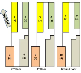
To demonstrate a practical importance of the proposed ap-proach, the prediction of total gas consumption of modeled office building heating is presented. An hourly prediction for the same building is described in details in [14]. The office building is located at Casaccia Research Centre of Italian National Agency for New Technologies, Energy and Sus-tainable Economic Development (ENEA). The structure is composed of three floors and a thermal plant in the base-ment. There are 41 offices of different size with a floor area ranging from 14 to 36m2, two electronic data processing
rooms each of about 20m2, four laboratories, one control room and two meeting rooms. Each office room has from one up to two occupants. For each room and laboratory, as thermal exchangers, there are fan-coils with on-off fan speed controlled by a proper thermostat with hysteresis equal to 1◦C. During winter, the thermal plant produces heat by a traditional natural gas boiler. This study is related only to heating during winter season. The thermal fluid circulation into fan-coil circuits is ensured by a triplet of centrifugal pumps. The building is equipped with an advanced moni-toring system collecting data from sensors of environmental conditions and electrical and thermal energy consumption.
In order to simulate testing data of sufficient sample sizes, a Matlab Simulink simulator based on Heat, Air and Moisture
Figure 2: Partitioning of F40 building zones. Num-bers denote the number of zones and numNum-bers in brackets denote corresponding number of fan-coils.
model for Building and Systems Evaluation [6] was used. In particular, the building was divided into ten controllable thermal zones according to different thermal behavior de-pending on solar radiation exposure. Therefore a zone con-sists of a group of rooms with similar climatic conditions and the same climate control policy. Figure 2 shows the division into thermal zones. Although there are 15 zones at all, those that do not have sensors and remotely controllable fan coils are not considered.
The gas consumption is derived by integration of the natural gas mass flow which depends directly from the discharge and return water temperature at the thermal plant and from the thermal plant efficiency. The fan-coils are modeled by theε-Number of Transfer Units (ε-NTU) method [4] which allows to derive the heat injected in the zones and the outlet water temperatures from known zone air temperatures, fan-coil inlet water flows and fan speeds. The inputs of the simulation are indoor temperature set points, current air temperatures inside the zones and external meteorological data. The summary of the inputs can be found in Table 1. The main task is to predict total gas consumption in the following 12 hours denoted asy(t).
The behavior of supply water temperature set point was con-trolled by a simple weather compensation rule. To excite the dynamics of the system in a proper degree, we also added a random component. The value of the temperature set point is Gaussian random number with standard deviation 4◦ C
Table 1: Summary of the network inputs
Inputs Names
x1(k) the value of the air temperature set point constant for the following 12 hours
x2(k) the value of the supply water temperature set point constant for the following 12 hours x3(k). . . x12(k) ten values of instantaneous air temperature in ten zones
x13(k). . . x19(k) arithmetic means of weather variables computed over last 12 hours
0 50 100 150 200 250
0.18 0.19 0.2 0.21 0.22 0.23 0.24 0.25 0.26 0.27 0.28
Number of network weights
Mean MSE
Feedforward NARX
Figure 3: Comparison of input selection for feedfor-ward network and proposed input and delay selec-tion for NARX.
in [19].
5.2.2
Results
The training data consisted of two simulated heating sea-sons, 2004/2005 and 2005/2006. To choose the output di-mensionality, neural networks with different numbers of re-gressors were tested on an independent validation data set 2006/2007. The testing errors of the method were computed on the 2008−2012 data sets, which are not used in any part of the predictor design process and are large enough to pro-vide valid estimate of the real prediction error.
The results are shown in Figure 3, where only testing error is depicted. The SBP of inputs and delays for NARX is compared to selection of inputs for common feed-forward network with the same number of hidden units, the same training algorithms and the other settings. To make the values on horizontal axis comparable, number of network weights is used. For three hidden units, maximum number of weights (without selection of inputs or delays) for feed-forward network is 57, while maximum number of weights for NARX is 237. This is why the graphs span different ranges on horizontal axis.
One can observe that without the selection of inputs and delays, NARX network with the original settings is signifi-cantly worse than the simple feedforward network (Wilcoxon sum-rank test,α= 0.05). On the other hand, if SBP is used, NARX network becomes better as the elimination proceeds until it permanently outperforms all feedforward networks
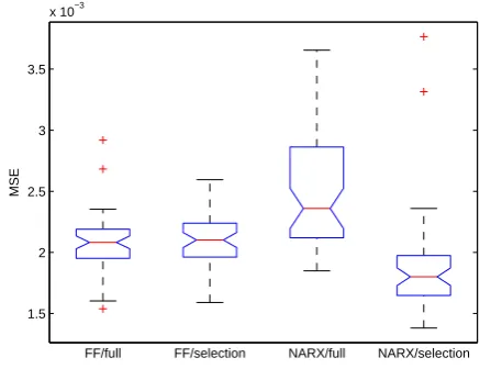
1.5 2 2.5 3 3.5
x 10−3
FF/full FF/selection NARX/full NARX/selection
MSE
Figure 4: Boxplots of MSE for feedforward network with full set of inputs (FF/full) and with selection of inputs (FF/selection) and for NARX network with full set of delays and inputs (NARX/full) and with selection of inputs and delays (NARX/selection).
of comparable number of weights. Moreover, one can see that the input selection for feedforward network causes a performance degradation. This demonstrates that the in-put and delays selection is much more important for NARX network than the input selection is for the feed-forward net-work. Although this result is obtained for a specific case of one particular application, it is highly probable that this will be also obtained for other data, because the NARX network has a more complex dynamics and its irrelevant connections cause higher prone to overfitting and smaller stability of the network.
Figure 3 does not consider a decision about number of in-puts and delays. Therefore, the final MSE obtained by min-imum validation error principle (see section 4) averaged over 100 runs is compared by boxplots in Figure 4. The figure supports the previous evidence that the pruning is more im-portant for NARX network than for feedforward network. Although NARX network is significantly worse for the origi-nal set of inputs and delays, it significantly outperforms the feedforward network if the pruning is used.
6.
CONCLUSIONS
The paper proposes an extension of SBP method to NARX networks. It shows that the method efficiently selects in-puts, simultaneously removes input and output delays and does not degrade the prediction performance. The approach is obviously not limited to NARX neural network, but is easily extendable to other networks. The extension would be straightforward. The network must be simulated on the data and the signal of connection, which is to be removed is collected for all data samples. Than the signal is replaced by its mean value computed from the collected signal.
For future, some practical implementation issues described in section 4 should be focused in more details. First, it should be examined, if and when the sensitivity based on hold-out error estimate (computed on validation data) brings some benefits to the resubstitution error estimate (computed on training data). Further, different methods for final de-cision about number of inputs and delays or different stop-ping condition for the backward search should be proposed. Finally, the influence of the use of the naive approach (con-sidering the same delays for all inputs) instead of compu-tationally more intensive exhaustive approach (considering and eliminating different delays from different inputs) should be examined.
7.
REFERENCES
[1] Abandah, G. A., Jamour, F. T., and Qaralleh,
E. A.Recognizing handwritten Arabic words using
grapheme segmentation and recurrent neural networks.International Journal on Document Analysis and Reecognition 17, 3 (SEP 2014), 275–291.
[2] Bauer, K. W., Alsing, S. G., and Greene, K. A.
Feature screening using signal-to-noise ratios.
Neurocomputing 31, 1ˆa ˘A¸S4 (2000), 29 – 44.
[3] Beghdad, R.Applying Fisher’s filter to select KDD
connections’ features and using neural networks to classify and detect attacks.Neural Network World 17, 1 (2007), 1–16.
[4] Bergman, T., Lavine, A., and Incropera, F.
Fundamentals of Heat and Mass Transfer, 7th Edition. John Wiley & Sons, Incorporated, 2011.
[5] Cun, Y. L., Denker, J. S., and Solla, S. A.
Advances in neural information processing systems 2. Morgan Kaufmann Publishers Inc., San Francisco, CA, USA, 1990, ch. Optimal Brain Damage, pp. 598–605.
[6] De Wit, M.HAMBASE: Heat, Air and Moisture
Model for Building And Systems Evaluation. Technische Universiteit Eindhoven, Faculteit Bouwkunde, 2006.
[7] Endisch, C., Hackl, C., and Schroeder, D.
Optimal brain surgeon for general dynamic neural networks. InProgress In Artificial Intelligence, Proceedings(2007), Neves, J and Santos, MF and Machado, JM, Ed., vol. 4874 ofLecture Notes in Artificial Intelligence, pp. 15–28. 13th Portuguese Conference on Artificial Intelligence, Guimaraes, Portugal, DEC 03-07, 2007.
[8] Giles, C., Lin, T., Horne, B., and Kung, S.The
past is important: A method for determining memory structure in NARX neural networks. InIEEE World Congress On Computational Intelligence(1998),
pp. 1834–1839.
[9] Hassibi, B., Stork, D., and Wolff, G.Optimal
brain surgeon and general network pruning. InNeural Networks, 1993., IEEE International Conference on
(1993), pp. 293–299 vol.1.
[10] He, Y.-J., Zhu, Y.-C., Duan, D.-X., and Sun, W.
Application of neural network model based on combination of fuzzy classification and input selection in short term load forecasting. InProceedings of 2006 International Conference on Machine Learning and Cybernetics, Vols 1-7 (2006), IEEE, pp. 3152–3156.
[11] Laine, T. I., and Bauer, K. W.Input feature
selection for automatic target recognition of temporal data.Military Operations Research 10, 2 (2005), 51–65.
[12] Leontaritis, I., and Billings, S.Input-output
parametric models for non-linear systems part I: deterministic non-linear systems.International Journal of Control 41, 2 (1985), 303–328.
[13] Ljung, L., Ed.System Identification (2Nd Ed.):
Theory for the User. Prentice Hall PTR, 1999.
[14] Macas, M., Lauro, F., Moretti, F., Pizzuti, S.,
Annunziato, M., Fonti, A., Comodi, G., and
Giantomassi, A.Sensitivity based feature selection
for recurrent neural network applied to forecasting of heating gas consumption. InInternational Joint Conference SOCO2014-CISIS2014-ICEUTE2014, vol. 299 of Advances in Intelligent Systems and Computing. Springer International Publishing, 2014, pp. 259–268.
[15] Mathworks. Neural Network Toolbox for Matlab
ver. 2012b, 2012.
[16] Moody, J.From Statistics to Neural Networks:
Theory and Pattern Recognition Applications. Springer-Verlag, 1994, ch. Prediction risk and neural network architecture selection.
[17] Moody, J. E.The effective number of parameters:
An analysis of generalization and regularization in nonlinear learning systems. InNIPS (1991), Morgan Kaufmann, pp. 847–854.
[18] Nelles, O.Nonlinear System Identification: From
Classical Approaches to Neural Networks and Fuzzy Models. Engineering online library. Springer, 2001.
[19] P.M.Ferreira, A.E.Ruano, S.Silva, and
E.Z.E.Concei¸c˜ao. Neural networks based predictive
control for thermal comfort and energy savings in public buildings.Energy and Buildings 55, 0 (2012), 238 – 251.
[20] Sheikhan, M.Generation of suprasegmental
information for speech using a recurrent neural network and binary gravitational search algorithm for feature selection.Applied Intelligence 40, 4 (2014), 772–790.
[21] Siegelmann, H., Horne, B., and Giles, C.