A Study Of Channel Estimation In Fast Fading Environments

196

A Study Of Channel Estimation In Fast Fading

Environments

Fatima Abdeen Farah Edris, Dr. Ashraf Gasim Elsid, Dr. Mohamed. H. M. Nerma

Abstract: This paper will be a study of two types of channel estimation techniques (LS & MMSE) that based on comb pilot insertion arrangement in fast fading channels environment which is consist of two types Rayleigh & Rician channel models, and a comparison between the two techniques will be done depending on different parameter and implement these into a simulation program which will be here MATLAB.

Index Terms: wireless channel, Fast fading, Rayleigh, Rician, comb pilot insertion, channel estimation, OFDM, LS, MMSE.

————————————————————

1. I

In wireless telecommunication environment, the signals that transfer through it are very susceptible to changing in amplitude and phase due to many factors such as multipath loss which is leading to phenomenon called fading. Fading refers to the fluctuations in signals strength when received at the receiver and Multipath fading is a common phenomenon that occurs in wireless signal transmission [1]. Wireless environments change quickly due to reflection, diffraction and scattering and thus introduce a complexity on the channel response. Due to the channel response that changed during the transmission and the received signal that distorted by the channel characteristics, the channel effect must be estimated and compensated in the receiver in order to recover the transmitted bits. Two main types of fading channel models are used here _in this paper_ Rayleigh and Rician channel models, and for channel estimation technique LS and MMSE will be used. Finally, implement of two channel estimation techniques in a simulation program, which will be the MATLAB program and the results will be shown later.

2. Overview of wireless communication

The performance of wireless communication systems is mainly governed by thewireless channel environment. As opposed to the typically static and predictable characteristics of a wired channel, the wireless channel is rather dynamic and unpredictable, which makes an exact analysis of the wireless communication system often difficult [2]. One of the most disturbing aspects in the wireless communication is fading, which is present when there are several multipath components and these components arrive at the receiver at slightly different times[3]. Two models of fast fading _Rayleigh & Rician_ channels will be studied and reviewed in order to understand the fading environments and its effect on the received channel response at the receiver.

3. Introduction to fading

Fading refers to the distortion that a carrier-modulated telecommunication signal experiences over certain propagation media. In wireless systems, fading is due to multipath propagation and is sometimes referred to as multipath induced fading [4]. It’s also known as the fluctuations in signals strength when received at the receiver [1]. To understand fading, it is essential to understand multipath. In wireless telecommunications, multipath is the propagation phenomenon that results in radio signals reaching the receiving antenna by two or more paths, however, causes of multipath include atmospheric ducting, ionosphere reflection and refraction, and reflection from terrestrial objects, such as mountains and buildings. The effects of multipath include constructive and destructive interference, and phase shifting of the signal. This distortion of signals caused by multipath is known as fading. In other words it can be said that in the real world, multipath occurs when there is more than one path available for radio signal propagation. The phenomenon of reflection, diffraction and scattering all give rise to additional radio propagation paths beyond the direct optical LOS (Line of Sight) path between the radio transmitter and receiver. Fading can be classified into two main types named as fast fading/small-scale fading, and slow fading/large-scale fading. Large-scale fading occurs as the mobile moves through a large distance, for example, a distance of the order of cell size and small-scale fading refers to rapid variation of signal levels due to the constructive and destructive interference of multiple signal paths (multi-paths) when the mobile station moves short distances [2].

Fast fading refers to the rapid fluctuations in the amplitude, phase, or multipath delays of the received signal, due to the interference between multiple versions of the same ______________________

 Fatima Abdeen FarahEdris is currently pursuing masters degree program in Telecommunication & Networking engineering in Future University, Sudan E-mail: [email protected].

 Supervisor: Dr. Ashraf Gasim Elsid Dean of faculty of telecommunication in future university.

 External supervisor: D. Mohamed. H. M. Nerma, faculty of electronics in Sudan university.

197 transmitted signal arriving at the receiver at slightly different

times. So, the time between the reception of the first version of the signal and the last echoed signal is called delay spread. The multipath propagation of the transmitted signal, which causes fast fading, is because of the three propagation mechanisms described as Reflection, diffraction and scattering. There are various models to describe statistical behavior of this phenomenon (Fading); the two common models that been used for fast fading are Rayleigh and Rice fading channel models [2].

A. Rayleigh fading channel model

Rayleigh fading occurs when there are multiple indirect paths between the transmitter and the receiver; which scatter, diffract or reflect the signal. Rayleigh fading is the specialized model for stochastic fading when there is no line of sight signal, and is sometimes considered as a special case of the more generalized concept of Rician fading. In Rayleigh fading, the amplitude gain is characterized by a Rayleigh distribution, it can be a useful model in heavily built-up city centers where there is no line of sight between the transmitter and receiver and many buildings and other objects attenuate, reflect, refract and diffract the signal. [5]. in which the fading coefficients are assumed to be zero-mean, complex Gaussian distributed. It occurs when no LOS path exists in between transmitter and receiver, but only have indirect path than the resultant signal received at the receiver will be the sum of all the reflected and scattered waves [2]. Probability density function for Rayleigh fading is:

fx x = x σ2e

−x2

2σ2 ₍₁₎

B. Rician fading channel model

When there is a strong dominate component is present, then the model must be follow the Rician distribution. The model of Rician fading is similar to the model of Rayleigh fading, unless that in Rician fading a strong dominant component is present [4]. It occurs when one of the paths, typically a line of sight signal, is much stronger than the others [5]. The pdf of Rician fading will be expressed as:

fx x x σ2e

−x2+c2 2σ2 _I

0 xc

σ2 (2) Where I0() is the modified Bessel function of the first kind with order zero and c is the strength of the direct component. In Rician fading, the amplitude gain is characterized by a Rician distribution. The Rician distribution is often described in terms of the Rician factor K, defined as the ratio between the deterministic signal power (from the direct path) and the diffuse signal power (from the indirect paths). K is usually expressed in decibels as [6]:

k dB = 10 log₁₀(c 2

2σ2) (3)

4.

C

During the past few years, the developments in digital communication are rapidly increasing to meet the ever increasing demand of higher data rates. Orthogonal frequency division multiplexing (OFDM) is a special case of multi-carrier transmission and it can accommodate high data rate requirement of multimedia based wireless systems. It has an edge over other frequency multiplexing techniques by using more densely packed carriers, thus achieving higher data rates using similar channels [7]. It is also a key technique for wireless communication because of its robustness for narrow

band interference, frequency selective fading and spectral efficiency [8]. The orthogonality of OFDM allows each subcarrier component of the received signal to be expressed as the product of the transmitted signal and channel frequency response at the subcarrier. Thus, the transmitted signal can be recovered by estimating the channel response just at each subcarrier [2]. So the characteristics of wireless signal changes as it travels from the transmitter antenna to the receiver antenna. These characteristics depend upon the distance between the two antennas, the paths taken by the signal and the environment around the path. In general, the power profile of the received signal can be obtained by convolving the power profile of the transmitted signal with the impulse response of the channel. Convolution in time domain is equivalent to multiplication in the frequency domain [5]. Therefore, the transmitted signal x, after propagation through the channel becomes y as in equation:

y = x ⊗ h + z (4) Where h is the channel response, z is noise and ⊗ is the circular convolution. Note that x, y, h, and z in the above equation are all functions of the signal frequency f. The objects located around the path of the wireless signal reflect the signal. Some of these reflected waves are also received at the receiver. Since each of these reflected signals takes a different path, it has a different amplitude and phase [5]. The estimation of channel is an important factor in OFDM system and it mostly done by three ways; training based channel estimation _it’s types will be discussed in details later_, blind channel estimation and semi blind channel estimation.

 Training-based (Pilot based) channel estimation: known symbols are transmitted specifically to aid the receiver’s channel estimation algorithms. Here, training symbols or pilot tone that are known a priori to the receiver, are multiplexed along with the data stream for channel estimation.

 Blind channel estimation: the receiver must determine the channel without the aid of known symbols. It is carried out by evaluating the statistical information of the channel and certain properties of the transmitted signals. Although higher-bandwidth efficiency can be obtained in blind techniques due to the lack of training overhead, the convergence speed and estimation accuracy are significantly compromised. Blind Channel Estimation has its advantage in that it has no overhead loss. It is only applicable to slowly time varying channels due to its need for a long data record.

 Semi blind channel estimation: is hybrid combination between blind and training technique, utilizing pilots and other natural constraints to perform channel estimation [5].

Pilot based channel estimation

198 estimation can be performed by either block type pilots or by

comb type pilots as will shown below. a) Block type pilots

In this type, the OFDM symbols of the channel estimation are transmitted periodically in time-domain and all subcarriers are used as pilots. It is particularly suitable for slow-fading radio channels.

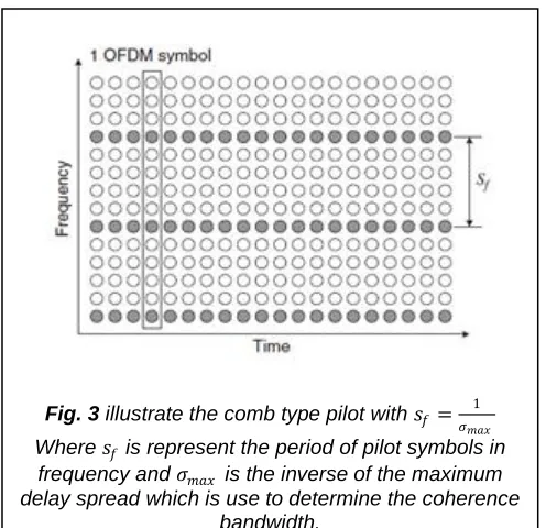
b) Comb type pilot

In this case, the pilot will be distributed uniformly within the OFDM symbol, and it suitable for fast fading channel which it is the study target field for this paper.

Where sf is represent the period of pilot symbols in frequency and σmax is the inverse of the maximum delay spread which is use to determine the coherence bandwidth. Since channel estimation is an integral part of OFDM systems, it is critical to understand the basis of channel estimation techniques for OFDM systems so that the most appropriate method are

based on least square (LS) and minimum mean-square error (MMSE) will be discussed in this paper.

A. LS channel estimation algorithm

The goal of the channel least square estimator (LS) is to minimize the square distance between the received signal and the original signal.

J H = Y − XH 2

= Y − XH H Y − XH (5) Y − YH_{XH − H}H_XH_{Y + H}H_XH_XH

Where (. )H_{is the conjugate transpose operator. By setting the} derivative of the function with respect to HH _{to zero}

∂J(H )

∂HH = −2(Y

H_X)∗_{+ 2(X}H_{XH )}∗

Now, the LS channel estimation as:

HLs = YXHX −1XHY = YX−1 (6) Where Y= XH

HLs = [k], k= 0,1,2,…,N-1.

Also HLs can be written for each subcarrier as:

H_Ls = Y X =

Y k X k

T

(7)

Where (. )T _{is the transpose operator and k = 0,1,2, … , N − 1.} The mean-square error (MSE) of the LS channel estimate is given as:

MSE_LS = E{ H − H_Ls H H − H_Ls } = E{ H − YX−1 H _{H − YX}−1 _}

= E X−1_Z H _X−1_{Z (8)} E = {ZH _XXH −1_Z}

= σz 2 σ²x

There, MSE is inversely proportional to the SNRσz2/σ²x, which implies that it may be subject to noise enhancement, especially when the channel is in a deep null. Due to its simplicity, however, the LS method has been widely used for channel estimation. Note that this simple LS estimator does not exploit the correlation of channel across subcarriers in frequency and across the OFDM symbols in time. Without using any knowledge of the statistics of the channel, the LS estimator can be calculated with very low complexity, but it has a high mean-square error since it does not take into account of the effect of noise on the signal [2]. This algorithm is very simple, because it is not considering any channel statistical parameters it is prone to the noise. So the performance is worse [9].

B. MMSE channel estimation algorithm

The MMSE channel estimation method finds a better (linear) estimate in terms of W in such a way that the MSE in Equation (9) is minimized. The orthogonality principle states that the estimation error vector e = H − H is orthogonal to H, such that:

Fig. 2 illustrate the block type pilot with 𝑠𝑡= 1 𝑓𝐷𝑜𝑝𝑝𝑙𝑒𝑟

Where 𝑠_𝑡 is represent the period of pilot symbols in time and 𝑓_{𝐷𝑜𝑝𝑝𝑙𝑒𝑟} is the Doppler frequency.

Fig. 3 illustrate the comb type pilot with 𝑠_𝑓 = 1 𝜎𝑚𝑎𝑥 Where 𝑠𝑓 is represent the period of pilot symbols in

frequency and 𝜎_𝑚𝑎𝑥 is the inverse of the maximum delay spread which is use to determine the coherence

199

J H = E e 2 _{= E H − H} 2 ₍₉₎

E{eHH_{} = E = {(H − H )H}H_} = E{(H − WH )HH_}

= E HHH _{− EW{ H H}H_{} (10)} R_HH− WR_{H H} = 0

Where RAB is the cross-correlation matrix of N X N matrices A and B (i.e., R_AB = E[ABH_{]), and H is the LS channel estimate} given as:

H = X−1_{Y = HX}−1_{Z (11)} Solving Equation (10) for W yields:

W = R_HH R−1_{H H} (12) Where RH His the autocorrelation matrix of H given as:

RH H = E HHH = E{ X−1_{Y X}−1_Y H_} = E{ H+X−1_{Z H + X}−1_Z H_}

= E HHH_+X−1_ZHH_+HZH _X−1 H_{+ X}−1_ZZH _X−1 H ₍₁₃₎ = E{HHH_{} + E{X}−1_ZZH _X−1 H_}

= E{HHH_{} +} σz2 σ²x

I

And R_HH is the cross-correlation matrix between the true channel vector and temporary channel estimate vector in the frequency domain. Using Equation (13), the MMSE channel estimate follows as:

H = WH = RHH RH−1 HH

R_HH+ σz2

σ²xI −1

(14)

MMSE estimator employs the second-order statistics of the channel conditions to minimize the mean-square error. To estimate the channel for data symbols, the pilot subcarriers must be interpolated. Popular interpolation methods include linear interpolation, second-order polynomial interpolation [2].

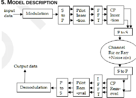
5.

M

The data symbols is first grouped and mapped according to the modulation technique [10]. Then it will be converted from serial to parallel for pilot inserting. For comb type pilot subcarrier arrangement, the Kp pilot signals Xp(m), m =0, 1, 2, …, Kp are uniformly inserted into X(k). That is, the total N subcarriers are divided into Kp groups, each with L= N/Kp adjacent subcarriers. In each group, the first subcarrier is used to transmit pilot signal. The OFDM signal modulated on the kth subcarrier is shown in two following equations, where:

X(k)= X(mL+l)

X(k) = Xp m , where l = 0

inf. Data, where l = 1,2, … , L − 1 (15) Where Xp(m) is the mth pilot carrier value [11]. After inserting pilots uniformly between the information data sequence, IDFT block _which is a kind of FFT used for digital data_ is used to transform the data sequence of length N fX(k) frequency domain signal into time domain signal fx(n) with the following equation:

x(n)= IDFT{X(k)} n= 0,1,2,….,N-1 = N−1X(k)

k=0 e 2πkn

N (16) where N is the DFT length [12]. Following IDFT block, guard

time, which is chosen to be larger than the expected delay spread is inserted to prevent inter-symbol interference.

This guard time includes the cyclic prefix which is a part of OFDM symbol in order to eliminate inter-carrier interference (ICI). The resultant OFDM symbol is given as follows:

x_f (n) = x N + n , n = −Ng, −Ng+ 1, … , −1

x n , n = 0,1 … , N − 1 (17) where Ng is the length of the guard interval [13][14]. The

transmitted signal xf (n) will pass through the Rayleigh and Rician fading channels with noise. In Rayleigh channel model the receiver receives a number of reflected and scattered waves. Because of the varying path lengths, the phases are random, and consequently, the instantaneous received power becomes a random variable. In the case of un modulated carrier, the transmitted signal at frequency ωc reaches the receiver via a number of paths, the ith path having an amplitude a_i, and a phase ∅_i. If assumed that there is no direct path or line-of sight (LOS) component, the received signal s(t) can be expressed as:

s t = Ni=1aicos⁡(ωct + ∅i) (18) where N is the number of paths. The phase ∅_i depends on the

varying path lengths, changing by 2π when the path length

200 changes by a wavelength. Therefore, the phases are uniformly

distributed over [0, 2π]. The envelope in this case has a Rayleigh density function given by equation (1) and the pdf of is governed by the scale parameter σ, the greater the scale parameter the wider distribution. In Rician channel model, the Rician distribution is observed when, in addition to the multipath components, there is an exist of direct path or line-of-sight component between the transmitter and the receiver. In the presence of such a path, the transmitted signal can be written as: s t = N−1i=1 aicos ωct +ωdit+∅i + c cos⁡(ωct + ωdt) (19)

Where the constant c is the strength of the direct component, ωdis the Doppler shift along the LOS path, and ωdi are the Doppler shifts along the indirect paths given by equation (18). The envelope in this case has a Rician probability density function given by equation (2) [6]. The distribution based on Rician is calculated according to the values using the corresponding scale parameter function in (2). In the receiver part, first the received signal must be converted from serial to parallel in order to remove the cyclic prefix and guard interval. The cyclic prefix would be of all zero samples transmitted in front of each OFDM symbol. It does not contain any useful data; it would be discarded at the receiver. The length of the guard interval should be longer than the time span of the channel, such that the OFDM symbol itself will not be distorted. Thus, by eliminating the guard interval, the impacts of intersymbol interference can be removed [9] and the signal is then will be equal to equation (4).Where z(n) is the noise, h(n) is the channel impulse response and ⊗ is circular convolution. yf n for − Ng≤ n ≤ N − 1 is equal to y n = yf n + Ng n = 0,1,2, … . . , N − 1 (20) Where y(n) is the received signal after CP removal and then y(n) [14] is sent to DFT block for defining Y(k) the following operation:

Y(k)= DFT{y(n)} k=0,1,2,…,N_1 =1

N y(n) N−1 k=0 e

2πkn

N (21) Assuming there is no ISI, the following equation will show the

relation of the resulting Y(k) to H(k) with the following equation:

Y(k) =X(k)H(k) +Z(k) (22) Where X is a matrix of size K x K with the elements of the

transmitted signals on its diagonal, Y is the received vector of size K x l, H is a channel frequency response of size K x 1 and Z is noise with zero-mean and variance. The noise Z is assumed to be uncorrelated with the channel H [24].

Y≜ Y[0]

⋮ Y[N−1]

=

X[0] ⋯ 0

⋮ ⋱ ⋮

0 ⋯ X[N−1]

H[0] ⋮ H[N−1]

+

Z[0] ⋮ Z[N−1]

(23)

Next block will be the channel estimation block, which _in this paper_ will be using the LS and MMSE channel estimation algorithms. The received pilot signal vector, Yp = [Yp(0),Yp(1), … Yp(Np−1)]T_{can be expressed as given by}

the following:

Yp=XpHp+Zp (24)

Where:

Xp=

X_p ⋯ 0

⋮ ⋱ ⋮

0 ⋯ Xp(Np−1)

(25)

Hp (k) is the frequency response of the channel at pilot sub-carriers and defined as Hp=[Hp(0),Hp(1), … Hp(Np−1)]T _,

and Zp=[Zp(0),Zp(1), … Zp(Np−1)]T _{is the noise vector in}

pilot subcarriers where [. ]T _{is a transpose operator [2]. The}

equations that used for both LS and MMSE is reported in details in the previously in equations (5) to (14). In channel estimation based on comb type pilot insertion, an interpolation technique is necessary in order to estimate channel at data carriers by using the channel information at pilot sub-carriers. The channel estimation at the data-carrier using linear interpolation is given by:

He k =He(mL+l)

Hp m+1 −Hp m l

L+Hp(m) (26)

The second-order interpolation results to be better than the linear interpolation. The channel estimated by second-order interpolation is given by:

He k =He(mL+l)

c₁H_p m−1 +c₀H_p m c₋₁H_p(m+1) (27)

Where

c1= α(α−1)

2

c0= α−1 α+1 ,α= l

N

c−1= α(α+1)

2

(28)

After estimate the channel at pilot sub-carriers by mean of channel estimation and data sub-carriers by using the channel information at pilot sub-carriers by mean of interpolation, the data now is ready to be un modulated after transfer it from parallel to serial in order to show the output signal at the end [8].

6.

S

The MATLAB environment provides an accurate simulation of the application in real world, the more details and parameters are defined the more accurate the simulation will be, thus providing strong results back to the conclusion. In this thesis, the attempt is to show comparison between LS & MMSE in term of MSE average and SNR using different modulations schemes.

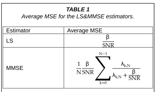
A. Implementing channel estimation in MATLAB MATLAB Program will perform the LS and MMSE channel estimation, respectively. It will calculate MSE & SNR for each and compare it in one plot. Next table will show equations that used to calculate average MSE.

TABLE 1

Average MSE for the LS&MMSE estimators.

Estimator Average MSE

LS β

SNR

MMSE 1

N

β

SNR

λ_k,N

λ_k,N+

β

SNR

N−1

k=0

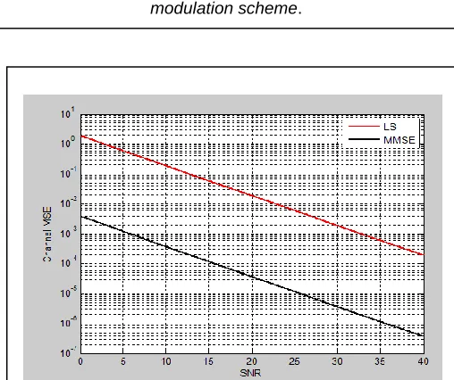
201 B. LS & MMSE Results

In figures 6, 7, 8, and 9, the comparison is done in order of calculating MSE average and SNR for both channel estimation algorithms. It shows that the MMSE has low MES & SNR and thus doing better performance than LS whatever the modulation used.

7.

C

In this thesis, a full review of fading channels model (Rayleigh & Rice), LS estimator and MMSE estimator is given. Rayleigh fading model is happens when no LOS path exists in between transmitter and receiver, but only have indirect path than the resultant signal received at the receiver will be the sum of all the reflected and scattered waves. Rician fading model will be appeared once the receiver receives one strong component which will be a line of sigh signal. MMSE estimator has a better performance than LS estimator in order of average MSE and SNR but it has a computational complexity so it use only in the low SNR environments. However, MMSE estimator will be used in systems that require precise measurement and time sensitive environments such as high speed communications systems. On modulation side, the results show that the M-QAM has a better performance for both channel estimation algorithms than M-PSK modulation.

Fig .6: the two techniques of channel estimation is used for 64 subcarriers, withcyclic prefix equal to 1/16 which

will be expected to be larger than maximum expected delay and using BPSK modulation.

Fig. 7: also the two techniques of channel estimation is used for 64 subcarriers, with cyclic prefix equal to 1/16

and using 16 QAM modulation.

Fig. 8:shows the two techniques will be used for 512 subcarriers with cyclic prefix 1/16 and using BPSK

modulation scheme.

Fig. 9: also done in 512 subcarriers with the same CP used for all previous simulations and using 16 QAM

202

8. Future Recommendations

In channel estimation, instead of use training-based channel estimation, the DFT-based channel estimation technique must be used because it was been derived to improve the performance of LS or MMSE channel estimation by eliminating the effect of noise outside the maximum channel delay. Technically, the performance of LS can be improved by using technique called Least Mean Square LMS. The LMS estimator uses one tap LMS adaptive filter at each pilot frequency. The first value is found directly through LS and the following values are calculated based on the previous estimation and the current channel output. For MMSE, although it has better performance the LS but its performance can be improved also by implementing Linear Minimum Mean Square LMMSE which has the best performance since it has the accurate channel statistical parameters and at high SNR, the performance of this algorithm is good.

9.

R

[1] Mr.P.Sunil Kumar1, Dr.M.G.Sumithra, Ms.M.Sarumathi, ―Performance evaluation of Rayleigh and Rician Fading Channels using M-DPSK Modulation Scheme in Simulink Environment‖, International Journal of Engineering Research and Applications (IJERA) ISSN: 2248-9622 www.ijera.com Vol. 3, Issue 3, pp.1324-1330, May-Jun 2013.).

[2] Yong Soo Cho, Chung-Ang University, Republic of Korea, Jaekwon Kim Yonsei University, Republic of Korea, Won Young Yang Chung-Ang University, Republic of Korea ,Chung G.Kang Korea University, Republic of Korea ―MIMO-OFDM WIRELESS COMMUNICATIONS WITH MATLAB‖, John Wiley & Sons (Asia) Pte Ltd, 2 Clementi Loop, # 02-01, Singapore 129809, 2010.

[3] Sanjiv Kumar, Department of Computer Engineering, BPS Mahila Vishwavidyalaya, Khanpur, Kalan-131305, India, E-mail: [email protected], P. K. Gupta Department of Computer Science and Engineering, Jaypee University of Information Technology, Waknaghat,

Solan – 173 234, India, E-mail:

[email protected], G. Singh Department of Electronics and Communication Engineering, Jaypee University of Information Technology, Waknaghat, Solan – 173 234, India, E-mail: [email protected], D. S. Chauhan, Uttarakhand Technical University, Deharadun, India, E-mail: [email protected] ―Performance Analysis of Rayleigh and Rician Fading Channel Models using Matlab Simulation‖, I.J. Intelligent Systems and Applications, 2013, 09, 94-102, Published Online August 2013 in MECS (http://www.mecs-press.org/), DOI: 10.5815/ijisa.2013.09.11.

[4] A. Sudhir Babu Associate Professor, Department of CSE, PVP Siddhartha Institute of Technology, Vijayawada, India, Dr. K.V Sambasiva Rao Professor and Principal MVR College of Engineering and Technology, Paritala, Vijayawada, India ―Evaluation of BER for AWGN, Rayleigh and Rician Fading Channels under Various Modulation Schemes‖ International Journal of Computer Applications (0975 – 8887) Volume 26– No.9, July 2011 23.

[5] AP / ECE Department, Sri Ramakrishna Engineering

College, Coimbatore, Tamil Nadu, India, Professor/ ECE Department, Sri Ramakrishna Engineering College, Coimbatore, Tamil Nadu, India, ―BER PERFORMANCE OF AWGN, RAYLEIGH AND RICIAN CHANNEL‖, International Journal of Advanced Research in Computer and Communication Engineering Vol. 2, Issue 5, May 2013.

[6] Gayatri S. Prabhu and P. Mohana Shankar, ―Simulation Of Flat Fading Using MATLAB For Classroom Instruction‖, Department of Electrical and Computer Engineering Drexel University 3141 Chestnut Street Philadelphia, PA 19104.

[7] Sajjad Ahmed Ghauri, [email protected], SherazAlam2, [email protected], M. Farhan Sohail3, [email protected], AsadAli Faizan Saleem, National University of Modern Languages, Islamabad, Pakistan, ―IMPLEMENTATION OF OFDM AND CHANNEL ESTIMATION USING LS AND MMSE ESTIMATORS‖, International Journal of Computer and Electronics Research [Volume 2, Issue 1, February 2013].

[8] Sonali Sahu & A.B. Nandgaonkar Dept. Electronics & Telecommunication, Dr.Babasaheb Ambedkar Technological University, Raigad,Maharashtra,India E-mail:[email protected],[email protected] , ―OFDM Comb-Type Channel Estimation using a MMSE Estimator‖, ISSN (PRINT) : 2320 – 8945, Volume -1, Issue -4, 2013.

[9] Vineetha Mathai, K. Martin Sagayam, ―Comparison And Analysis Of Channel Estimation Algorithms In OFDM Systems‖, INTERNATIONAL JOURNAL OF SCIENTIFIC & TECHNOLOGY RESEARCH VOLUME 2, ISSUE 3, MARCH 2013.

[10]van de Beek, J.J., Edfors, O., Sandell, M. et al. ―On channel estimation in OFDM systems‖. IEEE VTC’95, vol. 2, pp. 815–819 (July 1995).

[11]Hala M. Mahmoud Al-Quds University/ Department of Electronics Engineering, Jerusalem, Palestine Email: [email protected], Allam S. Mousa An-Najah-University/ Department of Electrical Engineering, Nablus, Palestine Email: [email protected], Rashid Saleem University of Manchester /School of Electrical and

Electronic Engineering, UK Email:

[email protected], ―Channel Estimation Based in Comb-Type Pilots Arrangement for OFDM System over Time Varying Channel‖, JOURNAL OF NETWORKS, VOL. 5, NO. 7, JULY 2010.

[12]S. Coleri, M. Ergen, A. Puri, and A. Bahai, ―Channel estimation techniques based on pilot arrangement in OFDM systems,‖ IEEE Trans. Broadcast., vol. 48, no. 3, pp. 223–229, Sep. 2002.

203 [14]Srishtansh Pathak and Himanshu Sharma Department of