www.ocean-sci.net/11/657/2015/ doi:10.5194/os-11-657-2015
© Author(s) 2015. CC Attribution 3.0 License.
Impact of currents on surface flux computations and their feedback
on dynamics at regional scales
A. Olita1, I. Iermano2, L. Fazioli1, A. Ribotti1, C. Tedesco1, F. Pessini1, and R. Sorgente1
1Institute for Coastal Marine Environment of the National Research Council, Oristano Section, Torregrande, Italy 2Department of Sciences and Technologies, Parthenope University, Naples, Italy
Correspondence to: A. Olita ([email protected])
Received: 4 December 2014 – Published in Ocean Sci. Discuss.: 8 January 2015 Revised: 24 July 2015 – Accepted: 21 August 2015 – Published: 31 August 2015
Abstract. A twin numerical experiment was conducted in the seas around the island of Sardinia (Western Mediterranean) to assess the impact, at regional and coastal scales, of the use of relative winds (i.e., taking into account ocean surface currents) in the computation of heat and momentum fluxes through standard (Fairall et al., 2003) bulk formulas. The Re-gional Ocean Modelling System (ROMS) was implemented at 3 km resolution in order to well resolve mesoscale pro-cesses, which are known to have a large influence in the dy-namics of the area. Small changes (few percent points) in terms of spatially averaged fluxes correspond to quite large differences of such quantities (about 15 %) in spatial terms and in terms of kinetics (more than 20 %). As a consequence, wind power inputP is also reduced by ∼14 % on average. Quantitative validation with satellite SST suggests that such a modification of the fluxes improves the model solution es-pecially in the western side of the domain, where mesoscale activity (as suggested by eddy kinetic energy) is stronger. Surface currents change both in their stable and fluctuating part. In particular, the path and intensity of the Algerian Cur-rent and of the Western Sardinia CurCur-rent (WSC) are impacted by the modification in fluxes. Both total and eddy kinetic en-ergies of the surface current field are reduced in the exper-iment where fluxes took into account the surface currents. The main dynamical correction is observed in the SW area, where the different location and strength of the eddies influ-ence the path and intensity of the WSC. Our results suggest that, even at local scales and in temperate regions, it would be preferable to take into account such a contribution in flux computations. The modification of the original code, sub-stantially cost-less in terms of numerical computation, im-proves the model response in terms of surface fluxes (SST
validated) and it also likely improves the dynamics as sug-gested by qualitative comparison with satellite data.
1 Introduction
un-τ =ρaCd|ua−us|(ua−us) (1)
Qs =ρaCpaCs|ua−us|(ta−ts) (2)
Ql =ρaLeCl|ua−us|(qa−qs), (3) whereρais the air density,uaandusare the vector velocities for air and sea surface respectively,ta−tsis the difference in temperature between air (at 10 m) and sea surface,qa−qsis the difference in humidity,CpaandLe are the specific heat of air and the latent heat of water evaporation respectively, whileCd,CsandClare the coefficient for momentum, sen-sible heat and latent heat transfer respectively.
Some recent papers provided evidence of a moderate but actual impact of such a modification on fluxes at global/oceanic scales. Kara et al. (2007) showed that the inclusion of ocean currents and dominant waves into the drag computation leads to a daily reduction of the drag of about 10 % at daily scale and for the entire globe, with large variability between mid-latitude (smaller impact) and tropics. Another model study (Dawe and Thompson, 2006) found that, for the North Pacific, heat fluxes and wind stress changed about 1–2 % at basin average, while local-ized changes (in the tropics) reached up to a 10 % reduction of both momentum flux and surface currents. In that study the wind power input to ocean surface is reduced by 27 %, quite in good accordance with previous findings of Duhaut and Straub (2006). In the Gulf Stream region, this reduction of the wind work was estimated to be around 17 % (Zhai and Greatbatch, 2007). Deng et al. (2009) also assessed the effect of coupling currents with winds. They found a 10 % change in surface currents when considering surface currents veloc-ities in the bulk formulas, quite in agreement with other au-thors.
All authors found that in the tropics such changes are more relevant than for mid-latitudes. This is a valid generalization for large scales, while an insight of what happens at mid-latitude and at regional and coastal scales was not provided yet. To address this issue we focused our attention in the seas around Sardinia (Western Mediterranean sea), which is a highly variable and dynamic area interested by several (sub-)mesoscale structures of different origin (Fuda et al., 2000; Puillat et al., 2002; Ribotti et al., 2004; Testor et al., 2005; Olita et al., 2013) and also affected by strong wind events characterized both by seasonality and high-frequency peaks.
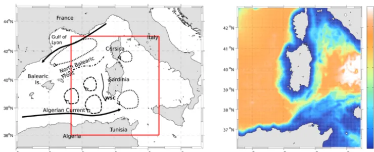
of this cyclonic gyre contributes to the formation of the North Balearic front (Fuda et al., 2000; Testor and Gascard, 2003; Olita et al., 2014) which represents the separation between the Atlantic water reservoir of the Algerian Basin and the saltier and denser waters of the Provençal basin (e.g. Olita et al., 2014). In a recent paper (Olita et al., 2013) we sug-gested, through the analysis of the outputs of a 3-D assimila-tive model, that the upwelling occurring along the SW Sar-dinian coast was pre-conditioned by the presence of a quasi-permanent southward current (Western Sardinian Current – WSC) whose origin was in part due to the approaching of an-ticyclonic eddies to the western Sardinia shelf. This was also supported by the findings of Pinardi et al. (2013) where the same current (they called Southerly Sardinia Current – SSC) is described as permanent at low-frequency scales (decadal) bordering a northern branch of the Atlantic water flow in the Western Mediterranean. In the southern part of the model do-main the Sardinian Channel connects Tyrrhenian and Alge-rian sub-basins. Here the AlgeAlge-rian Current (e.g. Millot et al., 1999) transports Atlantic water towards and across the Sicily Channel. North of Sardinia the Bonifacio Strait (∼ 15 km wide) separates Sardinia and Corsica and connects, with its narrow passage, Algero-Provençal and Tyrrhenian basins. Winds crossing the strait contribute to the generation of a wind-driven quasi-stable cyclonic gyre (Perilli et al., 1995; Millot et al., 1999) in the northern Tyrrhenian sea, east of Sardinia, that represents the most energetic mesoscale struc-ture of the northern Tyrrhenian sea (Iacono et al., 2013). All these different characteristics make this domain a good test case to study the impact of the inclusion of surface cur-rents on the surface fluxes and their feedback on circulation at regional and coastal scales.
al-Figure 1. Left: study area with toponyms and main circulation features as known from literature. Right: model domain and bathymetry. The bathymetry used is the GEBCO at 3000of resolution.
lowed to respect the suggested 1 : 3 ratio (e.g. Debreu and Blayo, 2008) between child and parent grid resolution, as well as to well resolve mesoscale processes (considering that the smallest Rossby radius of deformation for this area is of the order of about 10 km). Details on the model implementa-tion and experimental setup are provided in Sect. 2, together with information on the data and analyses performed. Two experiments were conducted, reproducing the circula-tion of the year 2012, with and without the contribucircula-tion of surface currents in the computation of the momentum and heat fluxes.
In Sect. 3 we validate the model vs. satellite SST and com-pare the outcomes of the two setups under different points of view. Finally, concluding remarks are drawn in Sect. 4.
2 Methods and data
2.1 Numerical model and experiments
The numerical model is an implementation of the Re-gional Ocean Modelling System (ROMS Shchepetkin and McWilliams, 2003, 2005) in its official release from Rut-gers (svn revision 705). Such a release of the code does not include an option to switch on/off the surface currents in the surface flux computations, so the original model code was modified in this sense. ROMS is a free surface, hydro-static, primitive equation, finite difference model widely used by the scientific community for many kinds of applications: large-scale circulation studies (e.g. Haidvogel et al., 2000), ecological modelling (Dinniman et al., 2003), coastal stud-ies (e.g. Wilkin et al., 2005; Iermano et al., 2012), sea-ice modelling and others. The model was implemented in the seas around Sardinia (Fig. 1) in a rectangular grid of 3 km resolution on the horizontal plane and 30 s terrain following levels. The equation distributing vertical levels allows a ro-bust description of surface and subsurface layers where most of the dynamical processes occur. Intermediate and deep layers are discretized with larger (on the vertical) meshes.
Bathymetry was derived from the General Bathymetric Chart of the Oceans (GEBCO), a global 30-arc-second database, and smoothed with a Shapiro filter to remove wavelengths of the order of the grid scale. This is in order to minimize the pressure gradient force error (PGFE) often caused by too steep bathymetric gradients. Stiffness parameters (rx0 and rx1, respectively 0.27 and 5.97) are well within the thresholds suggested by developers (ROMS user forum at https://www.myroms.org/forum/).
50 100 150 200 250 300 350 −1
−0.5 0
SST ACC
Days of run since 2012−01−01
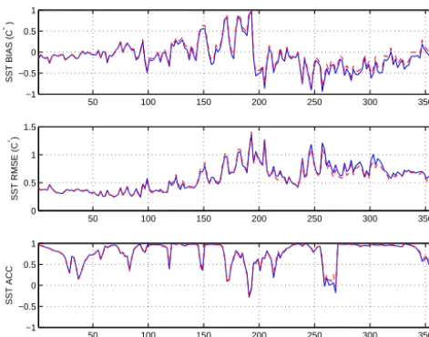
Figure 2. Top to bottom: BIAS, RMSE and ACC for BF (blue) and BFC (red dashed) experiments. Units for BIAS and RMSE are◦C, while ACC is dimensionless.
freshwater, momentum and heat fluxes by using the above-cited bulk formulas.
2.2 Experiments
Two experiments were performed: the Bulk Fluxes (BF) ex-periment did not include surface currents (so in Eqs. (1–3) theus term was neglected), while in Bulk Fluxes with Cur-rents (BFC) the flux computations interactively took into ac-count the surface currents reproduced by the model. This modification is quite straightforward when done in ROMS source code, just by taking care of the fact that currents and winds run on staggered grids, and therefore they have to be “interpolated” before performing subtraction. As a simple proxy for this, we averaged theiandi+1 velocity points for each windipoint and then we subtracted such quantities. The simulations were integrated for 1 year, to simulate the 2012 year with boundaries and surface forced by the above de-scribed analyses fields. Daily averaged fields are then saved in the output files.
The issue related to the data assimilation deserves a little dis-cussion. Considering that the model boundaries are provided by an assimilative model we think that for such a domain the information contained in the boundaries would propa-gate to the nested model without a substantial loss of infor-mation. On the contrary for larger off-line nested domains it was shown in literature (Vandenbulcke et al., 2006; Olita et al., 2012) that assimilation would be needed as informa-tion coming from boundaries quickly dissipates. Further, and maybe more important, in the present work we aim to ob-serve changes generated by different parametrizations of sur-face physics: for this reason we should not hide this signal with any statistical correction.
the model error in reproducing observed value of the con-sidered variable, ACC measures the ability of the model in reproducing anomalies of the SST signature detected by the satellite, partly overlooking their absolute value.
The three metrics are formulated as follows:
BIAS= 1
N
N
X
i=1
(obsi−modi), (4)
RMSE= v u u t 1
N
N
X
i=1
(obsi−modi)2, (5)
ACC=
N
P
i=1
(modi−obsi)(obsi−obsi)
s
N
P
i=1
(modi−obsi)2 N
P
i=1
(obsi−obsi)2
, (6)
where mod and obs are respectively modelled and observed values of the variable and the overbar stands for a long-term temporal average. In the present paper this long temporal av-erage is the AVHRR monthly climatology (1982–2008). The removal of the climatology allows to filter off the seasonal signal that otherwise would hide the response of this met-ric to the synoptic features. ACC is a dimensionless number ranging from−1 (worst) to+1 (best).
To further evaluate the quality of the two simulations, with particular reference to the dynamical features produced by the two experiments, we compared model outputs with synoptic observations of the sea surface observed in single swaths (Level 2) satellite images. Ocean colour and SST col-lected by MODIS sensors (on board of TERRA and AQUA satellites) were used for this purpose. Both typology of prod-ucts (optical and infrared derived respectively) can provide useful information on surface and subsurface structures. An example of such data comparison is presented in Sect. 3 which tries to emphasize differences between the two model setups and similarities with observed features.
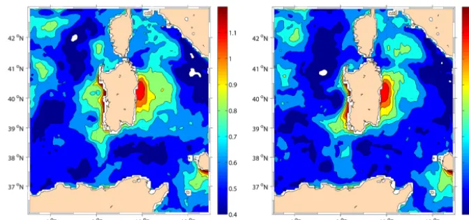
Figure 3. Map of SST RMSE (whole period) for BF (left) and BFC experiments. Units are◦C.
50 100 150 200 250 300 350
−10 −5
0x 10
−3
WS (N/m
2)
50 100 150 200 250 300 350
−1 0 1
SHF (W/m
2)
50 100 150 200 250 300 350
−2 0 2
LHF (W/m
2)
50 100 150 200 250 300 350
−4 −2 0 2
NHF (W/m
2)
Days since 2012−01−01
Figure 4. Top to bottom: wind stress, sensible, latent and net heat flux differences between the two experiments (BFC – BF). Negative sign indicates lower values for BFC in respect to BF.
part of the velocity field as already described, for example, in Olita et al. (2013). The time-averaged termu= hui +u0
represents the stable part of the flow, whileu0is its fluctuat-ing part. The fluctuatfluctuat-ing components can be used to describe both eddy kinetic energy (EKE=1/2(u02+v02)) and the Reynolds stress covariance term (RS=u0v0), i.e., the eddy momentum flux. Reynolds stress covariance shows where the turbulent part of the flow interacts with the mean flow, accel-erating or deflecting it from its mean direction (Greatbatch et al., 2010). It is likely that changes in surface parametriza-tion of surface fluxes would influence both the stable and the fluctuating part of the flow, but in different measure. This suggested us that the two should be investigated separately. Wind stress workP, which is defined as the product of wind stress τ by the surface ocean currentsus was computed in order to assess the differences in terms of wind power input
to the ocean between the two model experiments. At oceanic scales, including tropical areas, a reduction of about 20–30 % was recorded when the contribution of surface currents is considered (Duhaut and Straub, 2006; Hughes and Wilson, 2008).
3 Results and discussion
3.1 SST validation and intercomparison
Figure 2 shows the three time series for SST RMSE, BIAS and ACC metrics computed vs. the SST data.
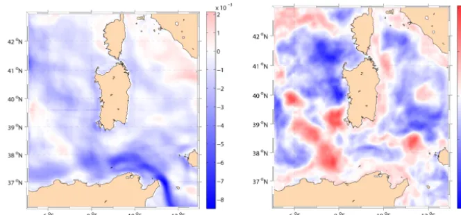
Figure 5. Difference map (BFC-BF) of the time-averaged wind stress (left) and net heat fluxes (right). Blue values indicate a BFC stress/heat lower than BF. Units are N m−2and W m−2respectively.
Figure 6. Total (left) and turbulent kinetic energy at surface. Red curve is for BF and green for BFC experiment.
3.2 Impact on surface fluxes
All the spatially integrated surface fluxes (momentum, sen-sible, latent and net heat, see Fig. 4) show an impact of the order of few percentage points (∼2 %) by averaging time se-ries values, but with a distinct high-frequency behaviour.
The small differences in terms of time series underneath quite large differences in space because of the very nature of the fluxes and the way they are computed (i.e., interactively during the model integration and with a feedback with ocean currents for BFC experiment). In this regard significant in-formation is provided by the time integrated wind stress dif-ference map shown in Fig. 5.
Such spatial differences, for wind stress, reach a low of −8×10⁻³N m−2 in the proximity of the southern bound-ary of the domain where the highly unstable Algerian Cur-rent flows. Another low is at the turning point of the West-ern Sardinia Current in the SW corner of Sardinia (−6× 10⁻³N m−2). Negative patches are quite dominant, as ex-pected. Positive patches are less present, reaching a maxi-mum of∼ 2×10⁻³N m−2and almost entirely located along the eastern Tyrrhenian coast. In percentage terms these spa-tial differences range between−15 % and+20 % on an an-nual basis, while they are obviously larger considering a
daily basis. The values of net heat flux difference (right panel of Fig. 5) are highly patchy and correlated with areas of im-proved model performances in terms of SST (as shown in Fig. 3). Near the western Sardinia coast (40◦N, 8◦E) the model shows the largest correction in terms of heat fluxes (negative blue patch).
3.3 Impact on the mean and turbulent surface circulation
As expected, wind stress changes generated significant mod-ifications in circulation and kinetics. Figure 6 shows time se-ries of total kinetic and eddy kinetic energy for the two exper-iments. It is evident that the introduction of the currents on stress computation (BFC) led to a large (spatially averaged) reduction of the kinetic energies at surface.
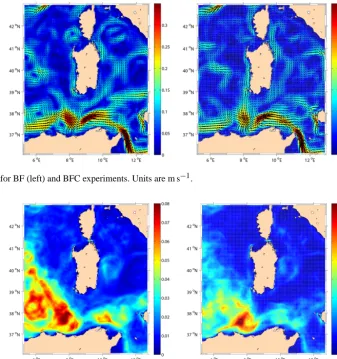
Figure 7. Mean flow for BF (left) and BFC experiments. Units are m s−1.
Figure 8. Eddie kinetic energy for BF (left) and BFC experiments. Units are m2s−2.
total one, with a maximum difference between the two ex-periments also during summer. Time-averaged maps of the above quantities provide an insight of the distribution of such differences.
The mean flow (Fig. 7) reveals some relevant change in terms of averaged path of the Western Sardinia Current which shows, surprisingly, a stronger signature in the BFC configuration. Some important change is evident in terms of mesoscale circulation: stable eddies footprints appearing in the SW side of the domain (with probable influence of boundaries) and west of Bonifacio strait, disappear in the averaged circulation field in favour of streams or a mean-dering feature. On the other side, EKE maps (Fig. 8) reveal that a large part of dynamical differences can be ascribed to the fluctuating part of the circulation as already argued from the time series. Eke values between the two model solu-tions shows an averaged reduction of about−23 % for BFC. The largest differences between the two EKE estimates are ascribed in the area of strongest mesoscale activity (Alge-rian Eddies area). Here a qualitative comparison of modelled fields vs. Level 2 single swath MODIS SST for 29 June 2012
(as an example) elucidates the differences between the two solutions in terms of mesoscale dynamics (Fig. 10).
In this figure the BFC solution better matches, in size and location, the large anticyclonic Eddy centred at about 38◦N, 8◦E, whose signature is also evident in the satellite image. BF solution on this case draws a less clear signature of the eddy and of the front on the east side of the eddy that, in the satellite image, seems also responsible for structuring the path of the WSC south of Sardinia. This is likely a recur-rent correction in the new model solution, as this area seems highly impacted by the flux correction both in terms of EKE and heat fluxes.
Figure 9. Reynolds stress covariance for BF (left) and BFC experiments. Units are m2s−2.
Figure 10. SST for BF (left), BFC experiments (right) and MODIS SST L2 (bottom panel) for 29 June 2012. Anticyclone is circled in black. Units are◦C degrees.
found (Olita et al., 2013) through an interannual experiment performed with a numerical assimilative model.
4 Conclusions
In the present work the impact of the surface currents in surface flux calculations at regional/coastal scales was assessed. To do this we performed 1-year long simulation with a new implementation of ROMS in the seas around Sardinia (Western Mediterranean Sea) by using two different
6oE 8oE 10oE 12oE 37oN
38oN 39oN
40oN 41oN
42oN
−6 −4 −2 0 2 4 x 10⁻³
Figure 11. Wind stress work difference (BFC – BF). Units are W m−2. Blue negative patches indicate where the wind power in-put is reduced by the feedback of currents on momentum fluxes.
domain, where mesoscale eddies are dominant.
Inclusion of surface currents determines relevant changes not only in dynamics but also in the prognosed surface temperature by means of the surface heat fluxes. Validation with satellite SST reveals that the solution is generally improved, even if only slightly in spatially averaged terms. Shelf-slope area west of central Sardinia largely benefits by the correction, while some areas shows questionable results, as for example the cyclonic area east of Bonifacio strait. Central and southern Tyrrhenian also show improvements in the BFC solution.
While quantitative metrics for SST reveal that net heat fluxes and resulting SST are improved, it is purely speculative to ascertain (i.e., not quantitatively validated) if, at these scales, the use of relative winds brings quality to the simulated dynamics or not. Comparison of synoptic satellite infrared and optic observations with modelled results did not solve the issue even if it provided some interesting hint in favour of the BFC solution.
Wind stress work, the product of wind stress and ocean surface currents, provides an insight of the wind power input to the ocean. Such an input is reduced for about 14 % as basin average. A difference map between the two estimates is shown in Fig. 11. The map shows larger differences on the left side, which is more windy and dynamic than the Tyrrhenian sea. The most interesting feature is the localized increase ofP in coincidence with the WSC (slightly shifted westward in BFC in respect to BF) justifying the increased signature of the WSC we detected in the averaged flow (cfr. Fig. 7).
The present study provides evidence that the contribution of surface currents should not be neglected in the
computa-tion of fluxes even at regional/coastal scales and in temperate regions. This is especially true and important for areas highly populated by (sub-)mesoscale features, which, in turn, are re-sponsible for the modulation of relevant physical-biological processes at sea as the triggering of primary production and the biomass redistribution and export.
Acknowledgements. Authors would like to thank the editor and the two anonymous reviewers who helped to substantially improve the manuscript.
This work has been funded by the Italian Flagship Project RITMARE and by the Italian Project PON-TESSA (C. U. PON01-02823), both funded by the Italian Ministry for Research – MIUR. Initial and boundary conditions as well as data for validation have been provided by the MyOcean data portal (http://www.myocean.eu) realized through EU projects MyOcean and MyOcean2 funded by VII FP SPACE (contracts 218812 and 283367).
Edited by: S. Carniel
References
Chapman, D. C.: Numerical treatment of cross-shelf open boundaries in a Barotropic Coastal Ocean Model, J. Phys. Oceanogr., 15, 1060–1075, doi:10.1175/1520-0485(1985)015<1060:NTOCSO>2.0.CO;2, 1985.
Dawe, J. T. and Thompson, L.: Effect of ocean surface currents on wind stress, heat flux, and wind power input to the ocean, Geo-phys. Res. Lett., 33, L09604, doi:10.1029/2006GL025784, 2006. Debreu, L. and Blayo, E.: Two-way embedding algorithms: a re-view, Ocean Dynam., 58, 415–428, doi:10.1007/s10236-008-0150-9, 2008.
Deng, Z., Xie, L., Liu, B., Wu, K., Zhao, D., and Yu, T.: Coupling winds to ocean surface currents over the global ocean, Ocean Model., 29, 261–268, doi:10.1016/j.ocemod.2009.05.003, 2009. Dinniman, M. S., Klinck, J. M., and Smith, W. O.: Cross-shelf exchange in a model of the Ross Sea circulation and biogeochemistry, Deep-Sea Res. Pt. II, 50, 3103–3120, doi:10.1016/j.dsr2.2003.07.011, 2003.
Duhaut, T. H. A. and Straub, D. N.: Wind stress dependence on ocean surface velocity: implications for mechanical en-ergy input to ocean circulation, J. Phys. Oceanogr., 36, 202, doi:10.1175/JPO2842.1, 2006.
Fairall, C. W., Bradley, E. F., Rogers, D. P., Edson, J. B., and Young, G. S.: Bulk parameterization of air-sea fluxes for Tropical Ocean-Global Atmosphere Coupled-Ocean Atmo-sphere Response Experiment, J. Geophys. Res., 101, 3747–3764, doi:10.1029/95JC03205, 1996.
Fairall, C. W., Bradley, E. F., Hare, J. E., Grachev, A. A., and Ed-son, J. B.: Bulk parameterization of air sea fluxes: updates and verification for the COARE algorithm, J. Climate, 16, 571–591, doi:10.1175/1520-0442(2003)016<0571:BPOASF>2.0.CO;2, 2003.
Hughes, C. W. and Wilson, C.: Wind work on the geostrophic ocean circulation: an observational study of the effect of small scales in the wind stress, J. Geophys. Res.-Oceans, 113, C02016, doi:10.1029/2007JC004371, 2008.
Iacono, R., Napolitano, E., Marullo, S., Artale, V., and Vetrano, A.: Seasonal variability of the tyrrhenian sea surface geostrophic cir-culation as assessed by altimeter data, J. Phys. Oceanogr., 43, 1710–1732, 2013.
Iermano, I., Liguori, G., Iudicone, D., Buongiorno Nardelli, B., Colella, S., Zingone, A., Saggiomo, V., and Ribera d’Alcalà, M.: Filament formation and evolution in buoyant coastal waters: Observation and modelling, Prog. Oceanogr., 106, 118–137, doi:10.1016/j.pocean.2012.08.003, 2012.
Kara, A. B., Metzger, E. J., and Bourassa, M. A.: Ocean current and wave effects on wind stress drag coefficient over the global ocean, Geophys. Res. Lett., 34, L01604, doi:10.1029/2006GL027849, 2007.
Lévy, M., Memery, L., and Madec, G.: The onset of a bloom after deep winter convection in the northwestern Mediterranean sea: mesoscale process study with a primitive equation model, J. Ma-rine Syst., 16, 7–21, 1998.
Marchesiello, P., McWilliams, J. C., and Shchepetkin, A.: Open boundary conditions for long-term integration of regional oceanic models, Ocean Model., 3, 1–20, doi:10.1016/S1463-5003(00)00013-5, 2001.
Mason, E., Molemaker, J., Shchepetkin, A. F., Colas, F., McWilliams, J. C., and Sangrà, P.: Procedures for offline grid nesting in regional ocean models, Ocean Model., 35, 1–15, doi:10.1016/j.ocemod.2010.05.007, 2010.
Millot, C., Gacic, M., Astraldi, M., and La Violette, P. E.: Circula-tion in the Western Mediterranean Sea, J. Marine Syst., 20, 423– 442, 1999.
Olita, A., Dobricic, S., Ribotti, A., Fazioli, L., Cucco, A., Dufau, C., and Sorgente, R.: Impact of SLA assimilation in the Sicily Chan-nel Regional Model: model skills and mesoscale features, Ocean Sci., 8, 485–496, doi:10.5194/os-8-485-2012, 2012.
Olita, A., Ribotti, A., Fazioli, L., Perilli, A., and Sor-gente, R.: Surface circulation and upwelling in the Sar-dinia Sea: A numerical study, Cont. Shelf. Res., 71, 95–108, doi:10.1016/j.csr.2013.10.011, 2013.
Olita, A., Sparnocchia, S., Cusí, S., Fazioli, L., Sorgente, R., Tin-toré, J., and Ribotti, A.: Observations of a phytoplankton spring bloom onset triggered by a density front in NW Mediterranean, Ocean Sci., 10, 657–666, doi:10.5194/os-10-657-2014, 2014. Penven, P., Debreu, L., Marchesiello, P., and McWilliams, J. C.:
Evaluation and application of the ROMS 1-way embedding
pro-time can near 3 years, J. of Marine Systems, 31, 245–259, 2002. Ribotti, A., Puillat, I., Sorgente, R., and Natale, S.: Mesoscale circu-lation in the surface layer off the southern and western Sardinia Island in 2000–2002, Chem. Ecol., 20, 345–363, 2004.
Shchepetkin, A. F. and McWilliams, J. C.: Quasi-monotone advection schemes based on explicit locally adaptive dis-sipation, Mon. Weather Rev., 126, 1541, doi:10.1175/1520-0493(1998)126<1541:QMASBO>2.0.CO;2, 1998.
Shchepetkin, A. F. and McWilliams, J. C.: A method for comput-ing horizontal pressure-gradient force in an oceanic model with a nonaligned vertical coordinate, J. Geophys. Res.-Oceans, 108, 3090, doi:10.1029/2001JC001047, 2003.
Shchepetkin, A. F. and McWilliams, J. C.: The regional oceanic modeling system (ROMS): a split-explicit, free-surface, topography-following-coordinate oceanic model, Ocean Model., 9, 347–404, doi:10.1016/j.ocemod.2004.08.002, 2005.
Testor, P. and Gascard, J.-C.: Large-scale spreading of deep wa-ters in the Western Mediterranean Sea by submesoscale coher-ent eddies, J. Phys. Oceanogr., 33, 75–87, doi:10.1175/1520-0485(2003)033<0075:LSSODW>2.0.CO;2, 2003.
Testor, P., Béranger, K., and Mortier, L.: Modeling the deep eddy field in the southwestern Mediterranean: the life cy-cle of Sardinian eddies, Gephys. Res. Lett., 32, L13602, doi:10.1029/2004GL022283, 2005.
Tonani, M., Pinardi, N., Fratianni, C., Pistoia, J., Dobricic, S., Pensieri, S., de Alfonso, M., and Nittis, K.: Mediterranean Forecasting System: forecast and analysis assessment through skill scores, Ocean Sci., 5, 649–660, doi:10.5194/os-5-649-2009, 2009.
Vandenbulcke, L., Barth, A., Rixen, M., Alvera-Azcarate, A., Ben Bouallegue, Z., and Beckers, J. M.: Study of the com-bined effects of data assimilation and grid nesting in ocean mod-els – application to the Gulf of Lions, Ocean Sci., 2, 213–222, doi:10.5194/os-2-213-2006, 2006.
Warner, J. C., Sherwood, C. R., Arango, H. G., and Signell, R. P.: Performance of four turbulence closure models implemented us-ing a generic length scale method, Ocean Model., 8, 81–113, doi:10.1016/j.ocemod.2003.12.003, 2005.
Wilkin, J. L., Arango, H. G., Haidvogel, D. B., Lichtenwalner, C. S., Glenn, S. M., and HedströM, K. S.: A regional ocean model-ing system for the long-term ecosystem observatory, J. Geophys. Res.-Oceans, 110, C06S91, doi:10.1029/2003JC002218, 2005. Zhai, X. and Greatbatch, R. J.: Wind work in a model of the