www.clim-past.net/10/1633/2014/ doi:10.5194/cp-10-1633-2014
© Author(s) 2014. CC Attribution 3.0 License.
Last interglacial model–data mismatch of thermal maximum
temperatures partially explained
P. Bakker1,2and H. Renssen1
1Earth and Climate Cluster, Department of Earth Sciences, VU University Amsterdam,
1081HV Amsterdam, the Netherlands
2now at: College of Earth, Ocean and Atmospheric Sciences, Oregon State University,
Corvallis, Oregon, USA
Correspondence to: P. Bakker ([email protected])
Received: 3 February 2014 – Published in Clim. Past Discuss.: 25 February 2014 Revised: 24 June 2014 – Accepted: 24 July 2014 – Published: 29 August 2014
Abstract. The timing of the last interglacial (LIG) thermal maximum across the globe remains to be precisely assessed. Because of difficulties in establishing a common temporal framework between records from different palaeoclimatic archives retrieved from various places around the globe, it has not yet been possible to reconstruct spatio-temporal vari-ations in the occurrence of the maximum warmth across the globe. Instead, snapshot reconstructions of warmest LIG conditions have been presented, which have an underlying assumption that maximum warmth occurred synchronously everywhere. Although known to be an oversimplification, the impact of this assumption on temperature estimates has yet to be assessed. We use the LIG temperature evolutions simu-lated by nine different climate models to investigate whether the assumption of synchronicity results in a sizeable overesti-mation of the LIG thermal maximum. We find that for annual temperatures, the overestimation is small, strongly model-dependent (global mean 0.4 ±0.3◦C) and cannot explain the recently published 0.67 ◦C difference between simulated and reconstructed annual mean temperatures during the LIG thermal maximum. However, if one takes into considera-tion that temperature proxies are possibly biased towards summer, the overestimation of the LIG thermal maximum based on warmest month temperatures is non-negligible with a global mean of 1.1 ±0.4◦C.
1 Introduction
The last interglacial period (LIG;∼130–116 thousand years before present [ka]) receives increasing attention because of the potential to constrain the impact of climate feed-backs such as increased melt rates of the major ice sheets in warm climates (Otto-Bliesner et al., 2006; Bakker et al., 2012, 2013; Stone et al., 2013) and to evaluate climate model performance for a warmer than present-day climate (Otto-Bliesner et al., 2006, 2013; Lunt et al., 2013; Masson-Delmotte et al., 2013). To facilitate the model–data compar-isons that are crucial in the evaluation of climate model per-formance, a number of compilations of reconstructed max-imum LIG temperatures have been produced (e.g. Kaspar et al., 2005; CAPE Last Interglacial Project Members, 2006; Clark and Huybers, 2009; Turney and Jones, 2010; McKay et al., 2011), based on a variety of different temperature prox-ies, retrieved from ice, marine and terrestrial archives. How-ever, because the LIG lies outside the time span covered by
14C dating, absolute chronological uncertainties for this
of LIG warming suggested by proxy-based reconstructions, whether using annual, or warmest month temperatures (Lunt et al., 2013; Bliesner et al., 2013). For example, Otto-Bliesner et al. (2013) recently performed a comparison be-tween a large number of continental and oceanic records and a LIG (130 ka) time-slice simulation with the CCSM3 model. They find that for the proxy sites in the Northern Hemisphere (NH) extratropical regions (30–90◦N), the re-constructed 1.71◦C annual mean temperature anomaly (with respect to pre-industrial; based on a combination of the com-pilations by Turney and Jones, 2010 and McKay et al., 2011) is considerably underestimated by the CCSM3 model (0.76◦C). This raises the question what causes this model– data mismatch of the LIG thermal maximum.
One partial reason for the mismatch could be that the syn-chronicity assumption underlying the compilations of the LIG thermal maximum is a non-negligible simplification. Several transient modelling experiments and proxy-based temperature reconstructions for both the present interglacial (PIG) and the LIG have shown that there are large regional differences in the timing of interglacial maximum warmth, of the order of several thousands of years (Renssen et al., 2009, 2012; Bakker et al., 2012; Govin et al., 2012; Langebroek and Nisancioglu, 2014). These temporal differences result from latitudinal and seasonal differences in the evolution of the orbital forcing, from the thermal inertia of the oceans and from a variety of feedbacks in the climate system, such as the presence of remnant ice sheets from the preceding deglacia-tion, changes in sea-ice cover, vegetadeglacia-tion, meridional over-turning strength and monsoon dynamics. Moreover, these complexities in the orbital forcing and its interaction with cli-mate feedbacks, cause seasonal differences in the timing of interglacial maximum warmth, e.g. the annual mean, summer or winter temperature maxima did not occur synchronously. As a consequence, a compilation of reconstructed LIG tem-peratures that combines LIG maximum temtem-peratures from different regions, seasons and climatic archives yields tem-perature anomalies that are larger than the maximum temper-atures that occurred at any given time during the LIG period. We use the results of transient LIG climate simulations performed by nine different climate models to (i) assess the magnitude and robustness of the possible overestima-tion of the LIG thermal maximum caused by the assump-tion of synchronicity in space and time, and (ii) inves-tigate the importance of the geographical region and the season over which the average is made. These results en-able us to discuss the degree to which the overestima-tion of the LIG thermal maximum resulting from the syn-chronicity assumption can explain the differences found in model–data comparison studies.
2 Method
LIG temperature time series from a total of nine dif-ferent climate models, ranging from earth system mod-els of intermediate complexity (EMIC) to general circu-lation models (GCM), have previously been compared in Bakker et al. (2013, 2014). A thorough description of the simulations and climate models can be found there, while an overview is given in Table 1. To investigate the possi-ble overestimation of the LIG thermal maximum, we calcu-late the temperature anomalies in two different ways: (i) we calculate regionally averaged temperature anomaly time se-ries and from that determine the warmest period (warmest-single-period; WSP) and (ii) we assume synchronicity of the LIG thermal maximum in space and time by calcu-lating for each individual model grid cell the largest LIG temperature anomaly and then combine these single-grid-cell maxima into regional averages (compilation-periods; CWP). In other words, the result of the warmest-single-period method can be regarded as a “real” estimate of the LIG thermal maximum, while the result from the compilation-warmest-periods is an analogue to the method used in proxy-based temperature compilations and yields an overestimated LIG thermal maximum that did not occur si-multaneously within the LIG.
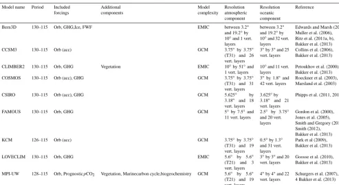
eval-Table 1. Overview of transient LIG climate simulations. For each simulation included in this study the model name is given, the period for which the simulation is performed (in thousands of years before present), the included forcings (Orb = orbital; acc = 10-fold acceleration of orbital forcing; GHG = Greenhouse gas concentrations; Ice = remnants of glacial continental ice sheets in NH; FWF = freshwater fluxes related to remnant ice sheets), components that are included in addition to the atmosphere, ocean and sea ice, the model complexity (EMIC = earth system model of intermediate complexity; GCM = general circulation model), the resolution of the atmospheric and oceanic model components and references to publications in which more details on the LIG simulations and the model specifics can be found.
Model name Period Included Additional Model Resolution Resolution Reference
forcings components complexity atmospheric oceanic
component component
Bern3D 130–115 Orb, GHG,Ice, FWF EMIC between 3.2◦
and 19.2◦by
10◦and 1 vert.
layers
between 3.2◦
and 19.2◦by
10◦and 32 vert.
layers
Edwards and Marsh (2005) Muller et al. (2006), Ritz et al. (2011a, b), Bakker et al. (2013)
CCSM3 130–115 Orb (acc) GCM 3.75◦by 3.75◦
(T31) and 26 vert. layers
3◦by 3◦and 25
vert. layers
Collins et al. (2006), Bakker et al. (2013)
CLIMBER2 130–115 Orb, GHG Vegetation EMIC 10◦by 51◦and
1 vert. layers
10◦and 11 vert.
layers
Petoukhov et al. (2000), Bakker et al. (2013)
COSMOS 130–115 Orb (acc), GHG GCM 3.75◦by 3.75◦
(T31) and 31 vert. layers
3◦by 1.8◦and
42 vert. layers
Roeckner et al. (2003), Marsland et al. (2003)
CSIRO 130–115 Orb (acc), GHG GCM 5.625◦ by
3.18◦ and 18
vert. layers
3.625◦by
3.18◦ and 21
vert. layers
Phipps et al. (2011, 2012)
FAMOUS 130–115 Orb, GHG GCM 5◦by 7.5◦and
11 vert. layers
2.5◦ by 3.75◦
and 20 vert. layers
Gordon et al. (2000), Jones et al. (2005), Smith and Gregory (2012), Smith (2012),
Bakker et al. (2013)
KCM 126–115 Orb (acc) GCM 3.75◦by 3.75◦
(T31) and 19 vert. layers
0.5◦by 1.3◦
and 31 vert. layers
Park et al (2009), Bakker et al. (2013)
LOVECLIM 130–115 Orb, GHG EMIC 5.6◦ by 5.6◦
(T21) and 3 vert. layers
3◦by 3◦and 20
vert. layers
Goosse et al. (2010), Bakker et al. (2013)
MPI-UW 128–115 Orb, PrognosticpCO2 Vegetation, Marinecarbon cycle,biogeochemistry GCM 5.6◦ by 5.6◦ (T21) and 19 vert. layers
4◦by 4◦and 22
vert. layers
Schurgers et al. (2007), 4 Bakker et al. (2013)
uate the robustness of the results. All model output in this study has been regridded to a common 1◦×1◦ resolution
and the temperatures used are atmospheric 2 m temperature anomalies with respect to pre-industrial values. All time series are 50-year averages in order to filter out decadal and sub-decadal variability. Determining the temporal resolution of a proxy-based LIG temperature compilation is difficult because the included temperature records typically cover a large range of temporal resolutions. Therefore, we test the importance of the temporal resolution by performing sen-sitivity experiments with 250-year and 2000-year averaged temperatures in addition to 50-year averages.
3 Results
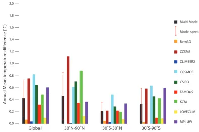
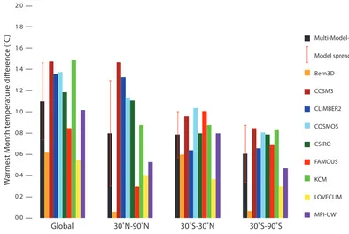
The calculations of the LIG thermal maximum based on the warmest-single-period and the compilation-warmest-periods methods, reveal large differences: between the individual models, between different geographical regions and between the annual mean and warmest month temperature anomalies. On a global scale the differences in the estimated LIG ther-mal maximum temperature another-maly between the two dif-ferent methods are 0.4◦C for MMM annual temperatures, with an inter-model spread of 0.3◦C (1σ; Fig. 1 and
Ta-ble 2). For smaller geographical regions, the MMM differ-ences in annual temperatures during the LIG thermal max-imum are smaller in case of the tropics and SH extratrop-ics (0.2±0.2◦C and 0.3±0.3◦C, respectively) and larger for the NH extratropics (0.5±0.4◦C) while the inter-model spread becomes larger in all three regions in comparison with the mean. The causes of the regional differences in the assessed overestimation of annual mean LIG maximum warmth will be discussed in the final part of the results sec-tion.
For warmest month temperature anomalies we find that the differences between the two methods used to calcu-lated MMM LIG maximum temperature anomalies are much larger compared to the calculations based on annual temper-atures. For warmest month temperatures the difference be-tween the warmest-single-period and compilation-warmest-periods methods is globally 1.1±0.4◦C and regionally
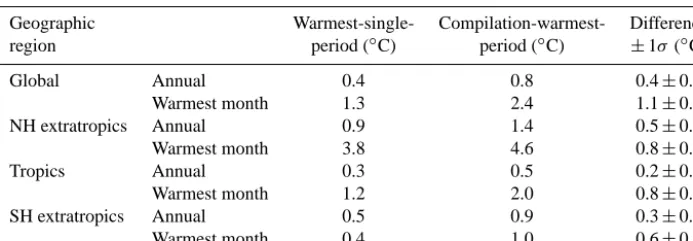
Table 2. MMM overestimation of LIG maximum warmth. Simulated MMM LIG temperature anomalies (◦C) for the single-warmest-period and for compilation-warmest-periods. Values are given for annual mean temperatures and for temperatures of the warmest month as well as for four different geographical regions: global, NH extratropical (30–90◦N), tropics (30◦S–30◦N) and SH extratropical (90–30◦S). The last column gives the difference between the two methods and the inter-model spread (1σ). All values are anomalies compared to simulated pre-industrial temperatures. The warmest-single-period is the largest 50-year temperature anomaly found in the regionally averaged temper-ature evolution. On the other hand, the compilation-warmest-periods follows from a regional average over the highest 50-year tempertemper-ature anomalies found in each individual grid cell within that region. Calculations are performed for the 130–120 ka period of the LIG.
Geographic Warmest-single- Compilation-warmest- Difference
region period (◦C) period (◦C) ±1σ(◦C)
Global Annual 0.4 0.8 0.4±0.3
Warmest month 1.3 2.4 1.1±0.4
NH extratropics Annual 0.9 1.4 0.5±0.4
Warmest month 3.8 4.6 0.8±0.5
Tropics Annual 0.3 0.5 0.2±0.1
Warmest month 1.2 2.0 0.8±0.2
SH extratropics Annual 0.5 0.9 0.3±0.3
Warmest month 0.4 1.0 0.6±0.3
not simply follow the month of highest insolation. We find that over the NH extratropical continents the warmest month is generally June, for the NH extratropical oceans it is August and for the SH extratropical oceans February (Fig. 3). In the low latitudes the land–sea differences are also apparent, but on top of that, monsoon dynamics and other local processes appear to play an important role in shaping the seasonal tem-perature evolution.
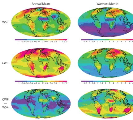
The quantification of the potential overestimation of LIG maximum warmth reveals the importance of the spatial do-main over which the calculations are performed. The rela-tively large differences found for the globally averaged LIG thermal maximum based on warmest month temperatures are a direct consequence of the large contrast in the evolution of orbitally forced summer insolation between the high latitudes of the NH and the SH (Bakker et al., 2013). The annual global warmest-single-period is characterised by a MMM warming of∼1◦C over the mid-to-high latitudes of the NH compared to simulated pre-industrial values, a∼0.5◦C warming over the SH mid-latitude continents and over Antarctica (Fig. 4). In contrast, the African and Indian monsoon regions show a∼1◦C cooling compared to pre-industrial. If this is com-pared to the annual compilation-warmest-periods, we will not find a cooling in the monsoon regions and the warm-ing in the mid-to-high latitudes of both hemispheres is on average∼0.5◦C larger than the single-warmest-period tem-perature anomalies. Over the tropical oceans the differences between both methods are small. For warmest month temper-atures we find a different picture. Because of the contrasting LIG evolution of summer insolation for the NH and the SH, the warmest month global warmest-single-period is charac-terised by a warming of∼5◦C over the NH continents and
∼2◦C over the NH oceans while for the same period sim-ulated SH warmest month temperatures are∼0.5◦C below pre-industrial values. In contrast, the
compilation-warmest-periods temperatures in the SH show a 0.5◦C warming for warmest month temperatures, especially over the continents. NH warming in the compilation-warmest-periods is also larger than in the global warmest-single-period.
Multi-Model-Mean
Model spread (1σ)
Bern3D
CCSM3
CLIMBER2
COSMOS
CSIRO
FAMOUS
KCM
LOVECLIM
MPI-UW 2.0
1.8
1.6
1.4
1.2
1.0
0.8
0.6
0.4
0.2
0.0
A
nnual M
ean t
emper
atur
e diff
er
enc
e (
˚C)
Geographical Region
Global 30˚N-90˚N 30˚S-30˚N 30˚S-90˚S
Figure 1. Overestimation of LIG maximum warmth taking into account simulated annual mean temperatures. Differences between the compilation-warmest-periods and the warmest-single-period methods to calculate the simulated LIG thermal maximum annual mean tem-perature anomalies (◦C). Results are given for four different geographical regions and for MMM temperature differences (black with 1σ inter-model spread in red) and for the nine individual model runs.
changes in the meridional overturning circulation (Bakker et al., 2013); changes that arise as internal climate variabil-ity, with the exception of the Bern3D simulation that includes prescribed meltwater fluxes from remnants of NH continen-tal ice sheets from the preceding deglaciation. Changes in the meridional overturning circulation have a large impact on surface temperatures and can therewith act to strongly synchronise simulated LIG maximum temperatures over ex-tensive parts of the globe, thus decreasing the difference be-tween the warmest-single-period and compilation-warmest-periods temperatures.
4 Discussion
We have shown that in climate models the synchronicity as-sumption potentially results in a sizeable overestimation of the LIG thermal maximum. However, to assess the possible overestimation of the LIG thermal maximum, two arbitrary choices have been made. First, we selected the 130–120 ka period to represent the LIG in this analysis, and second, we applied a 50-year average to the simulated temperature time series. To test the robustness of the results with respect to these two choices, we performed two additional sets of calculations in which we (1) used a 130–125 ka period in-stead of 130–120 ka and (2) used 250-year and 2000-year
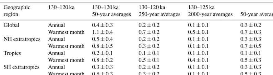
averaged temperature time series instead of 50-year aver-ages. We find that the resulting MMM overestimation of the LIG thermal maximum becomes smaller if the LIG period is decreased to 130–125 ka (annual mean global difference of 0.3±0.2◦C instead of 0.4±0.3◦C), in case the time averag-ing is increased to 250-year (annual mean global difference of 0.3±0.2◦C instead of 0.4±0.3◦C) and even more so if the time averaging is increased to 2000-year (annual mean global difference of 0.1±0.1◦C instead of 0.4±0.3◦C; see Table 3 for more details and regional differences). The ex-planation is that decreasing the length of the analysis pe-riod, limits the insolation differences between the two hemi-spheres. Furthermore, larger temporal averages smooth out an increasing part of the spatial differences related to inter-nal variability, again decreasing spatio-temporal differences in the LIG temperature maximum. Nonetheless, the main fea-tures described above appear robust.
Table 3. Robustness of MMM overestimation of LIG maximum warmth. Calculated MMM overestimation of LIG maximum warmth (mean ±1σ;◦C) and the dependence of the results on the two main choices: time frame of the LIG period over which the calculations are performed (130–120 ka in columns 3, 4 and 5; 130–125 ka in column 6) and the temporal resolution of the simulated temperature time series (50-year averages in columns 3 and 6; 250-year averages in column 4; 2000-year averages in column 5). Values are given for annual mean temperatures and for temperatures of the warmest month as well as for four different geographical regions: global, NH extratropics (30–90◦N), tropics (30◦S–30◦N) and SH extratropical (90–30◦S).
Geographic 130–120 ka 130–120 ka 130–120 ka 130–125 ka
region 50-year averages 250-year averages 2000-year averages 50-year averages
Global Annual 0.4±0.3 0.2±0.2 0.1±0.1 0.3±0.2
Warmest month 1.1±0.4 0.7±0.2 0.5±0.1 0.7±0.3
NH extratropics Annual 0.5±0.4 0.2±0.2 0.1±0.1 0.3±0.3
Warmest month 0.8±0.5 0.3±0.2 0.1±0.1 0.7±0.5
Tropics Annual 0.2±0.1 0.1±0.1 0.1±0.1 0.1±0.1
Warmest month 0.8±0.2 0.5±0.1 0.4±0.1 0.5±0.3
SH extratropics Annual 0.3±0.3 0.2±0.2 0.1±0.1 0.3±0.3
Warmest month 0.6±0.3 0.3±0.2 0.1±0.1 0.5±0.3
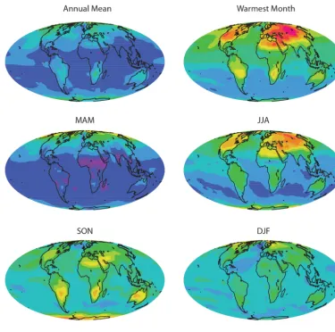
warmest month compilation-warmest-periods (Fig. 5). Note that calculating the single-warmest-period over a large spa-tial domain, for instance a global average, for a specific set of months, for instance MAM, is meaningless because such an average would combine temperatures from largely differ-ent seasons (see also Fig. 3). We find that the compilation-warmest-periods temperature anomalies in the NH extratrop-ics are largest in JJA while they are largest in SON over the SH extratropical continents and part of the Southern Ocean. Interpreting the seasonal temperature anomalies in terms of the potential overestimation of the LIG thermal maximum is difficult, because it is the temperature anomaly in combi-nation with spatial differences in the occurrence of the tem-perature anomalies within the LIG that determine the size of the overestimation. Notwithstanding this limitation, the max-imum seasonal temperature anomalies that occurred during the 130–120 ka period as found in the MMM provide a good reference for future studies into the seasonality aspects of different temperature proxies.
To assess if the calculated overestimation of the LIG thermal maximum can explain part of the reported model– data mismatch (Lunt et al., 2013; Otto-Bliesner et al., 2006, 2013), we compare our results with the findings of Otto-Bliesner et al. (2013). They performed a number of sen-sitivity experiments with the CCSM3 climate model, with for instance different orbital parameters, and compared their results with proxy-based compilations of Turney and Jones (2010) and McKay et al. (2011), including both continental and oceanic temperature reconstructions. Otto-Bliesner et al. (2013) show that the smallest LIG thermal maximum model– data differences are found in a model simulation forced with 130 ka forcings (orbital parameters and greenhouse-gas con-centrations). Moreover, the model–data difference is found to be smaller if the comparison is performed at the proxy locations instead of taking the model average over all grid cells within the geographical domain under consideration
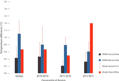
(see Otto-Bliesner et al., 2013, for thorough model and sce-nario description). Nonetheless, a global mean model–data temperature difference of 0.67◦C is found (anomalies of 0.98 and 0.31◦C with respect to preindustrial values in the recon-structions and simulations, respectively). The MMM over-estimation of LIG thermal maximum annual mean temper-atures presented here (0.4±0.3◦C) can only provide a
par-tial explanation of this model–data difference (Fig. 6). We do note that for a number of individual models an annual mean global overestimation of over 0.6◦C is found. If the 0.98◦C global temperature increase during the LIG thermal maximum (OtBliesner et al., 2013) would be biased to-wards the warmest month, the calculated global 1.1±0.4◦C overestimation resulting from the synchronicity assumption could potentially fully explain the model–data difference of 0.67◦C (Fig. 6). Also for specific geographical regions like the tropics, we find that the model–data difference can poten-tially be explained by the calculated overestimation for the warmest month temperatures (simulated 0.8±0.2◦C with respect to a 0.50◦C model–data difference). In the NH ex-tratropics the simulated MMM of 0.8±0.5◦C is compara-ble to the 0.67◦C model–data difference; however, the
inter-model spread is large with values ranging from∼0.05 up to∼1.5◦C. For the SH extratropical regions, the calculated
Multi-Model-Mean
Model spread (1σ)
Bern3D
CCSM3
CLIMBER2
COSMOS
CSIRO
FAMOUS
KCM
LOVECLIM
MPI-UW 2.0
1.8
1.6
1.4
1.2
1.0
0.8
0.6
0.4
0.2
0.0
W
ar
mest M
on
th t
emper
atur
e diff
er
enc
e (
˚C)
Geographical Region
Global 30˚N-90˚N 30˚S-30˚N 30˚S-90˚S
Figure 2. Overestimation of LIG maximum warmth taking into account simulated warmest month temperatures.Differences between the compilation-warmest-periods and the warmest-single-period methods to calculate the simulated LIG thermal maximum warmest month temperature anomalies (◦C). Results are given for four different geographical regions and for MMM temperature differences (black with 1σ inter-model spread in red) and for the nine individual model runs.
Jan Feb Mar Apr May Jun Jul Aug Sep Oct Nov Dec
Figure 3. Multi-model mean months of LIG maximum warmth. Month during which 50-year averaged LIG maximum warmth is found. Median of the nine different models is taken as the multi-model mean and for the calculations of LIG maximum warmth we applied the compilation-warmest-periods method, e.g. maximum LIG temperatures per individual grid cell.
Otto-Bliesner et al. (2013) and the transient climate simu-lations analysed here, can potentially impact the comparison between both studies. Most notably because it is unlikely that in reality the climate was in equilibrium with maximum LIG NH summer insolation and greenhouse-gas concentrations as
implied by the set-up of Otto-Bliesner et al. (2013). However, because this maximum LIG radiative forcing was only ap-plied for 1 ky, we deem it unlikely to be of large importance for the presented comparison between both studies.
Figure 4. Spatial differences in quantified overestimation of LIG maximum temperatures for annual mean and warmest month temperatures. Map of MMM LIG maximum temperature anomalies (◦C) compared to pre-industrial for the warmest-single-period (WSP, top row), the compilation-warmest-periods (CWP, middle row) and the difference between the two methods (CWP–WSP, bottom row). Maps are presented for both simulated annual mean and warmest month temperatures. Warmest-single-period results shown here are based on the globally averaged single-warmest-period. Note the differences and the non-linearity in the colour scales.
the early LIG (Bakker et al., 2013, 2014), with most mod-els showing SH maximum LIG temperatures <120 ka and NH maximum LIG temperatures>125 ka. Furthermore, the LIG simulations are not all forced with identical climate forc-ings. Most notably, the CCSM3 and KCM simulations lack transient greenhouse-gas concentration changes, the Bern3D simulation includes remnants of glacial ice sheets and related meltwater fluxes, the CLIMBER2 and MPI-UW simulations include dynamic calculations of vegetation feedbacks while the other models do not and finally the CCSM3, COSMOS, CSIRO and KCM include an accelerated orbital forcing with a potential impact on the simulated internal variability of the climate. The lack of remnant ice sheets during the early LIG in the simulations (except the Bern3D simulation) potentially impacts the heterogeneity of the thermal maximum (Renssen
Figure 5. Spatial differences in LIG maximum temperatures (◦C) compared to pre-industrial for DJF, MAM, JJA and SON temperatures following the compilation-warmest-periods (CWP) methodology.
5 Conclusions
With transient simulations covering the LIG period by nine different climate models, we investigate whether the assump-tion of synchronicity in space and time of the LIG ther-mal maximum that has to be made in compiling recon-structed LIG temperatures, results in a sizable overestima-tion of the LIG thermal maximum. For annual mean tempera-tures, the calculated overestimation is small, strongly model-dependent (global MMM of 0.4◦C with a ±0.3◦C
inter-model spread) and cannot explain the 0.67◦C model–data
difference described by Otto-Bliesner et al. (2013). How-ever, if reconstructed LIG temperatures would prove to be partly biased towards the warm season, the calculated global and tropical overestimation of the LIG thermal maximum based on simulated warmest month temperatures (global MMM 1.1±0.4◦C; tropics MMM 0.8±0.2◦C) can poten-tially fully explain the global and tropical model–data differ-ences described by Otto-Bliesner et al. (2013), 0.67◦C and
MMM Annual Mean
MMM Warmest Month
Model spread (1σ)
Model-Data Difference 2.0
1.8
1.6
1.4
1.2
1.0
0.8
0.6
0.4
0.2
0.0
Temper
atur
e diff
er
enc
e (
˚C)
Geographical Region
Global 30˚N-90˚N 30˚S-30˚N 30˚S-90˚S
Figure 6. Comparison of calculated overestimation of the LIG thermal maximum and reported LIG model–data mismatch. The calculated MMM overestimation of annual mean (black) and warmest month temperatures (blue;◦C) during the LIG thermal maximum, including inter-model spread (1σ; red) compared with the model–data mismatch (red) reported by Otto-Bliesner et al. (2013). The calculated MMM overestimation is illustrated by the differences between the compilation-warmest-periods and the warmest-single-period methods. Values are given for four different geographical regions. The model–data mismatch is based on a combination of terrestrial and oceanic data, comparison at proxy locations only and on a CCSM3 simulation forced with 130 ka forcings (see for details Otto-Bliesner et al., 2013).
Acknowledgements. This is Past4Future contribution no. 63. The
research leading to these results has received funding from the Eu-ropean Union’s Seventh Framework programme (FP7/2007–2013) under grant agreement no. 243908, “Past4Future. Climate change – Learning from the past climate” The authors gratefully acknowl-edge all groups for providing the simulated LIG temperature time series, in particular Sylvie Charbit, Matthias Gröger, Uta Krebs-Kanzow, Madlene Pfeiffer, Steven Phipps, Stefan Ritz, Emma Stone and Vidya Varma.
Edited by: D. Fleitmann
References
Bakker, P., Van Meerbeeck, C. J., and Renssen, H.: Sensitivity of the North Atlantic climate to Greenland Ice Sheet melting during the Last Interglacial, Clim. Past, 8, 995–1009, doi:10.5194/cp-8-995-2012, 2012.
Bakker, P., Stone, E. J., Charbit, S., Gröger, M., Krebs-Kanzow, U., Ritz, S. P., Varma, V., Khon, V., Lunt, D. J., Mikolajewicz, U., Prange, M., Renssen, H., Schneider, B., and Schulz, M.: Last interglacial temperature evolution – a model inter-comparison, Clim. Past, 9, 605–619, doi:10.5194/cp-9-605-2013, 2013. Bakker, P., Masson-Delmotte, V., Martrat, B., Charbit, S., Renssen,
R., Gröger, M., Krebs-Kanzow, U., Lohmann, G., Lunt, D. J., Pfeiffer, M., Phipps, S. J., Prange, M., Ritz, S. P., Schulz,
M., Stenni, B., Stone, E. J., and Varma, V.: Temperature trends during the Present and Last interglacial periods – A multi-model-data comparison – Quat. Sci. Rev., 99, 224–243, doi:10.1016/j.quascirev.2014.06.031, 2014.
CAPE Last Interglacial Project Members: Last Interglacial Arctic warmth confirms polar amplification of climate change, Quat. Sci. Rev., 25, 1383–1400, 2006.
Clark, P. U. and Huybers, P.: Global change: Interglacial and future sea leve, Nature, 462, 856–857, 2009.
Collins, W. D., Bitz, C. M., Blackmon, M. L., Bonan, G. B., Bretherton, C. S., Carton, J. A., Chang, P., Doney, S. C., Hack, J. J., Henderson, T. B., Kiehl, J. T., Large, W. G., McKenna, D. S., Santer, B. D., and Smith, R. D., The Community Climate System Model Version 3 (CCSM3), J. Clim., 19, 2122–2143, 2006.
Edwards, N. R. and Marsh, R.: Uncertainties due to transport-parameter sensitivity in an efficient 3-D ocean-climate model, Clim. Dyn., 24, 415–433, 2005.
Goosse, H., Brovkin, V., Fichefet, T., Haarsma, R. J., Huybrechts, P., Jongma, J. I., Mouchet, A., Selten, F. M., Barriat, P., Campin, J., Renssen, H., Roche, D. M., Timmermann, A. and Opsteegh, J. D., Description of the Earth system model of intermediate complexity LOVECLIM version 1.2, Geosci. Mod. Dev., 3, 309– 390, 2010.
of SST, sea ice extents and ocean heat transports in a version of the Hadley Centre coupled model without flux adjustments, Clim. Dyn., 16, 147–168, 2000.
Govin, A., Braconnot, P., Capron, E., Cortijo, E., Duplessy, J.-C., Jansen, E., Labeyrie, L., Landais, A., Marti, O., Michel, E., Mos-quet, E., Risebrobakken, B., Swingedouw, D., and Waelbroeck, C.: Persistent influence of ice sheet melting on high northern lat-itude climate during the early Last Interglacial, Clim. Past, 8, 483–507, doi:10.5194/cp-8-483-2012, 2012.
Gregory, J. M., Dixon, K. W., Stouffer, R. J., Weaver, A. J., Driess-chaert, E., Eby, M., Fichefet, T., Hasumi, H., Hu, A., Jungclaus, J. H., Kamenkovich, I. V., Levermann, A., Montoya, M., Mu-rakami, S., Nawrath, S., Oka, A., Sokolov, A. P., and Thorpe, R. B.: A model intercomparison of changes in the Atlantic ther-mohaline circulation in response to increasing atmospheric CO2
concentration, Geophys. Res. Lett., 32, 1944–8007, 2005. Gröger, M., Maier-Reimer, E., Mikolajewicz, U., Schurgers, G.,
Vizcaino, M. and Winguth, A., Vegetation-climate feedbacks in transient simulations over the last interglacial (128 000 – 113 000 yr BP). In F. Sirocko, M. Claussen, M. S. Goni, and T. Litt (Eds.), The climate of past interglacials (pp. 563–572). Amsterdam: El-sevier, 2007.
Jones, P. D., Gregory, J., Thorpe, R., Cox, P., Murphy, J., Sexton, D. and Valdes, P., Systematic Optimisation and climate simulations of FAMOUS, a fast version of HadCM3, Clim. Dyn., 25, 189– 204, 2005.
Kaspar, F., Kühl, N., Cubasch, U., and Litt, T.: A model-data com-parison of European temperatures in the Eemian interglacial, Geophys. Res. Lett., 32, L11703, doi:10.1029/2005GL022456, 2005.
Kopp, R. E., Simons, F. J., Mitrovica, J. X., Maloof, A. C., and Oppenheimer, M.: Probabilistic assessment of sea level during the last interglacial stage, Nature, 462, 863–867, 2009.
Langebroek, P.M. and Nisancioglu, K. H.: Simulating last inter-glacial climate with NorESM: role of insolation and greenhouse gases in the timing of peak warmth, Clim. Past, 10, 1305–1318, doi:10.5194/cp-10-1305-2014, 2014.
Leduc, G., Schneider, R., Kim, J. H., and Lohmann, G.: Holocene and Eemian sea surface temperature trends as revealed by alkenone and Mg/Ca paleothermometry, Quat. Sci. Rev., 29, 989–1004, 2010.
Lohmann, G., Pfeiffer, M., Laepple, T., Leduc, G., and Kim, J.-H.: A model-data comparison of the Holocene global sea surface temperature evolution, Clim. Past, 9, 1807–1839, doi:10.5194/cp-9-1807-2013, 2013.
Lunt, D. J., Abe-Ouchi, A., Bakker, P., Berger, A., Braconnot, P., Charbit, S., Fischer, N., Herold, N., Jungclaus, J. H., Khon, V. C., Krebs-Kanzow, U., Langebroek, P. M., Lohmann, G., Nisan-cioglu, K. H., Otto-Bliesner, B. L., Park, W., Pfeiffer, M., Phipps, S. J., Prange, M., Rachmayani, R., Renssen, H., Rosenbloom, N., Schneider, B., Stone, E. J., Takahashi, K., Wei, W., Yin, Q., and Zhang, Z. S.: A multi-model assessment of last interglacial tem-peratures, Clim. Past, 9, 699–717, doi:10.5194/cp-9-699-2013, 2013.
Marsland, S. J., Haak, H., Jungclaus, J. H., Latif, M. and Röske, F., The Max-Planck-Institute global ocean/sea ice model with or-thogonal curvilinear coordinates, Ocean Mod., 5, 91–127, 2003. Masson-Delmotte, V., Schulz, M., Abe-Ouchi, A., Beer, J., Ganopolski, A., Rouco, J. G., Jansen, E., Lambeck, K.,
Luter-bacher, J., Naish, T., Osborn, T., Otto-Bliesner, B., Quinn, T., Ramesh, R., Rojas, M., Shao, X., and Timmermann, A.: Informa-tion from Paleoclimate Archives, in: Climate Change 2013: The Physical Science Basis, Contribution of Working Group I to the Fifth Assessment Report of the Intergovernmental Panel on Cli-mate Change, Cambridge University Press, Cambridge, United Kingdom and New York, NY, USA, 2013.
McKay, N. P., Overpeck, J. T., and Otto-Bliesner, B. L.: The role of ocean thermal expansion in Last Interglacial sea level rise, Geophys. Res. Lett., 38, L14605, doi:10.1029/2011GL048280, 2011.
Muller, S. A., Joos, F., Edwards, N. R., and Stocker, T. F., Wa-ter Mass Distribution and Ventilation Time Scales in a Cost-Efficient, Three-Dimensional Ocean Model, J. Clim., 19, 5479– 5499, 2006.
Otto-Bliesner, B. L., Brady, E. C., Clauzet, G., Tomas, R., Levis, S., and Kothavala, Z.: Last Glacial Maximum and Holocene Climate in CCSM3, J. Climate, 19, 2526–2544, 2006.
Otto-Bliesner, B. L., Rosenbloom, N., Stone, E. J., McKay, N. P., Lunt, D. J., Brady, E. C., and Overpeck, J. T.: How warm was the last interglacial? New model - data comparisons, Philosophical Transactions of the Royal Society A: Mathematical, Phys. Engin. Sci., 371, 1–20, 2013.
Park, W., Keenlyside, N., Latif, M., Stroh, A., Redler, R., Roeckner, E. and Madec, G., Tropical Pacific Climate and Its Response to Global Warming in the Kiel Climate Model, J. Clim., 22, 71–92, 2009.
Petoukhov, V., Ganopolski, A., Brovkin, V., Claussen, M., Eliseev, A., Kubatzki, C. and Rahmstorf, S., CLIMBER-2: a climate sys-tem model of intermediate complexity. Part I: model description and performance for present climate, Clim. Dyn., 16, 1–17, 2000. Phipps, S. J., Rotstayn, L. D., Gordon, H. B., Roberts, J. L., Hirst, A. C. and Budd, W. F., The CSIRO Mk3L climate system model version 1.0 - Part 1: Description and evaluation, Geosci. Mod. Dev., 4, 483–509, 2011.
Phipps, S. J., Rotstayn, L. D., Gordon, H. B., Roberts, J. L., Hirst, A. C. and Budd, W. F., The CSIRO Mk3L climate system model version 1.0 - Part 2: Response to external forcings, Geosci. Mod. Dev., 5, 649–682, 2012.
Renssen, H., Seppa, H., Heiri, O., Roche, D. M., Goosse, H., and Fichefet, T.: The spatial and temporal complexity of the Holocene thermal maximum, Nature Geosci., 2, 411–414, 2009. Renssen, H., Seppa, H., Crosta, X., Goosse, H., and Roche, D. M.: Global characterization of the Holocene Thermal Maximum, Quat. Sci. Rev., 48, 7–19, 2012.
Ritz, S. P., Stocker, T. F. and Joos, F., A coupled dynamical ocean-energy balance atmosphere model for paleoclimate studies, J. Clim., 24, 349–375, 2011.
Ritz, S. P., Stocker, T. F. and Severinghaus, J. P., Noble gases as proxies of mean ocean temperature: sensitivity studies using a climate model of reduced complexity, Quat. Sci. Rev., 30, 3728– 3741, 2011.
Schmidt, G. A., Jungclaus, J. H., Ammann, C. M., Bard, E., Bra-connot, P., Crowley, T. J., Delaygue, G., Joos, F., Krivova, N. A., Muscheler, R., Otto-Bliesner, B. L., Pongratz, J., Shindell, D. T., Solanki, S. K., Steinhilber, F. and Vieira, L. E. A., Climate forc-ing reconstructions for use in PMIP simulations of the last mil-lennium (v1.0), Geosci. Mod. Dev., 4, 33–45, 2012.
Schneider, B., Leduc, G., and Park, W.: Disentangling sea-sonal signals in Holocene climate trends by satellite-model-proxy integration, Paleoceanography, 25, PA4217, doi:10.1029/2009PA001893, 2010.
Schurgers, G., Mikolajewicz, U., Gröger, M., Maier-Reimer, E., Vizcaíno, M. and Winguth, A., The effect of land surface changes on Eemian climate, Clim. Dyn., 29, 357–373, 2007.
Smith, R. and Gregory, J., The last glacial cycle: transient simula-tions with an AOGCM, Clim. Dyn., 38, 1545–1559, 2012.
Smith, R., The FAMOUS climate model (version XFXWB and XFHCC): description update to version XDBUA, Geosci. Mod. Dev., 5, 269–276, 2012.
Stone, E. J., Lunt, D. J., Annan, J. D., and Hargreaves, J. C.: Quan-tification of the Greenland ice sheet contribution to Last Inter-glacial sea level rise, Clim. Past, 9, 621–639, doi:10.5194/cp-9-621-2013, 2013.
Turney, C. S. M. and Jones, R. T.: Does the Agulhas Current amplify global temperatures during super-interglacials?, J. Quat. Sci., 25, 839–843, 2010.