https://doi.org/10.5194/npg-24-307-2017 © Author(s) 2017. This work is distributed under the Creative Commons Attribution 3.0 License.
Subvisible cirrus clouds – a dynamical system approach
Elisa Johanna Spreitzer1,a, Manuel Patrik Marschalik1,b, and Peter Spichtinger1 1Institute for Atmospheric Physics, Johannes Gutenberg University Mainz, Mainz, Germany anow at: Institute for Atmospheric and Climate Science, ETH Zurich, Zurich, Switzerland bnow at: Fritz-Haber-Institut der Max-Planck-Gesellschaft, Berlin, Germany
Correspondence to:Peter Spichtinger ([email protected]) Received: 21 December 2015 – Discussion started: 19 January 2016 Revised: 23 May 2017 – Accepted: 26 May 2017 – Published: 30 June 2017
Abstract.Ice clouds, so-called cirrus clouds, occur very fre-quently in the tropopause region. A special class are sub-visible cirrus clouds with an optical depth lower than 0.03, associated with very low ice crystal number concentrations. The dominant pathway for the formation of these clouds is not known well. It is often assumed that heterogeneous nu-cleation on solid aerosol particles is the preferred mecha-nism although homogeneous freezing of aqueous solution droplets might be possible, since these clouds occur in the low-temperature regime T <235 K. For investigating sub-visible cirrus clouds as formed by homogeneous freezing we develop a reduced cloud model from first principles, which is close enough to complex models but is also sim-ple enough for mathematical analysis. The model consists of a three-dimensional set of ordinary differential equations, and includes the relevant processes as ice nucleation, dif-fusional growth and sedimentation. We study the forma-tion and evoluforma-tion of subvisible cirrus clouds in the low-temperature regime as driven by slow vertical updraughts (0< w≤0.05 m s−1). The model is integrated numerically and also investigated by means of theory of dynamical sys-tems. We found two qualitatively different states for the long-term behaviour of subvisible cirrus clouds. The first state is a stable focus; i.e. the solution of the differential equations performs damped oscillations and asymptotically reaches a constant value as an equilibrium state. The second state is a limit cycle in phase space; i.e. the solution asymptotically approaches a one-dimensional attractor with purely oscilla-tory behaviour. The transition between the states is charac-terised by a Hopf bifurcation and is determined by two pa-rameters – vertical updraught velocity and temperature. In both cases, the properties of the simulated clouds agree rea-sonably well with simulations from a more detailed model,
with former analytical studies, and with observations of sub-visible cirrus, respectively. The reduced model can also pro-vide qualitative interpretations of simulations with a complex and more detailed model at states close to bifurcation qualita-tively. The results indicate that homogeneous nucleation is a possible formation pathway for subvisible cirrus clouds. The results motivate a minimal model for subvisible cirrus clouds (SVCs), which might be used in future work for the devel-opment of parameterisations for coarse large-scale models, representing structures of clouds.
1 Introduction
for-mation of ice crystals requires high supersaturation (see e.g. Koop et al., 2000; Hoose and Möhler, 2012) and diffusional growth of ice crystals is quite slow in the low-temperature regime (T <235 K), cirrus clouds mostly exist in a thermo-dynamic state far away from equilibrium. Thus, in contrast to liquid clouds, which approximately coincide with their (super-)saturated environment, for ice clouds there can be a continuous transition from clear air over very low ice crystal number concentrations to thick cirrus clouds with high mass and number concentrations. Cirrus clouds with optical thick-nessτ <0.03 constitute a special class, so-called subvisible cirrus clouds (SVCs; Sassen and Dodd, 1989). These clouds are difficult to measure; remote-sensing techniques such as lidar (e.g. Immler et al., 2008b) or occultation observations (e.g. Wang et al., 1996) are used to detect these very thin cirrus clouds. Only few in situ measurements of subvisible cirrus clouds are available, suggesting very low values in ice crystal number concentrations (Froyd et al., 2010; Kübbeler et al., 2011). Global observations from satellites (Wang et al., 1996; Stubenrauch et al., 2010; Hoareau et al., 2013) as well as observations with stationary lidar systems (Sassen and Campbell, 2001; Hoareau et al., 2013) show frequen-cies of occurrence of about 10–20 % in the extra-tropics; in the tropics the frequency of occurrence is much higher (up to 50 %; see e.g. Wang et al., 1996). For subvisible clouds, a net warming of the Earth–atmosphere system is almost certain, since the albedo effect is almost negligible. Our knowledge of subvisible cirrus clouds is quite limited. Since the ice crys-tal number concentration in SVCs is very low, the question about the dominant formation mechanism is still pending. At cold temperatures (T <235 K), where pure ice clouds oc-cur, two different formation mechanisms are generally possi-ble, namely heterogeneous nucleation at solid aerosol parti-cles (e.g. Dufour, 1861; aufm Kampe and Weickmann, 1951; Hosler, 1951) and homogeneous freezing of aqueous solu-tion droplets (Sassen and Dodd, 1989; Koop et al., 2000). For subvisible cirrus, Kärcher and Solomon (1999) stated that both nucleation mechanisms might be possible; in contrast, Jensen et al. (2001) and Froyd et al. (2010) clearly suggested that the dominant mechanism must be heterogeneous nucle-ation. However, analytical investigations by Kärcher (2002) indicated that also pure homogeneous nucleation might be possible.
In the present study we focus on the formation of SVCs by homogeneous freezing of aqueous solution droplets (here-after: homogeneous nucleation). We study the formation and evolution of SVCs in an air parcel that is lifted in slow vertical upward motions (0< w≤0.05 m s−1), as typical for synoptic-scale motions in the extra-tropics (e.g. along warm fronts; see Kemppi and Sinclair, 2011) or in slow as-cent regions in the tropics, for example driven by Kelvin waves (Immler et al., 2008a). We concentrate on the cold-temperature regime (T <235 K); thus, we exclude the possi-bility of liquid origin ice clouds (Krämer et al., 2016; Wernli et al., 2016), i.e. freezing of pre-existing cloud droplets at
states close to water saturation. This is not a strong limita-tion since the microphysical properties of ice clouds stem-ming from mixed-phase clouds are quite different, with high ice crystal number and mass concentrations and higher opti-cal depths (Luebke et al., 2016).
For the investigation of subvisible cirrus clouds we de-velop a parcel model to which we apply numerical and an-alytical tools. The model is developed on the basis of an evo-lution equation for mass distributions of ice crystals, includ-ing a description of microphysical processes based on former work (Spichtinger and Gierens, 2009). We take into account the relevant processes for ice microphysics, i.e. ice nucle-ation, ice crystal growth due to diffusion of water vapour, and sedimentation of ice crystals. We make use of some ap-propriate simplifications in order to obtain a reduced model consisting of an autonomous system of ordinary differential equations (ODEs), suitable for the application of analytical tools. The variables of the system are ice crystal mass and number concentration, respectively, as well as relative hu-midity with respect to ice. Thus, we have to investigate a three-dimensional autonomous system of ODEs.
To study the qualitative behaviour of the model we use concepts from theory of dynamical systems (see e.g. Ver-hulst, 1996; Argyris et al., 2010; Hirsch et al., 2013). The qualitative properties of the system near equilibrium states are relevant for the overall behaviour of the system. The stability of these equilibrium states can be investigated by applying perturbations after linearisation and is determined by the eigenvalues of the linearised system. Some theorems are available in order to transfer the qualitative behaviour of the linearised systems to the full nonlinear system. For the characterisation of more complex attractors, e.g. limit cy-cles, more sophisticated approaches must be used. For in-stance, limit cycles can be determined using Poincaré sec-tions (Argyris et al., 2010). Investigasec-tions of cloud models as dynamical systems were carried out for liquid and mixed-phase clouds (Hauf, 1993; Wacker, 1992, 1995, 2006) as well as for cloud–aerosol–precipitation systems (Koren and Fein-gold, 2011; Feingold and Koren, 2013). For pure ice clouds such investigations have not been carried out yet. In contrast to clouds involving liquid phase, which are close to thermo-dynamic equilibrium (i.e. RH∼100 %), we have to consider relative humidity as a system variable, which adds another equation to the system and makes the analysis more challeng-ing. The mathematical characterisation of the reduced model allows for a better understanding of the interaction of differ-ent nonlinear processes and the impact of external forcings such as vertical updraughts. Finally, the qualitative analysis could be used in future work as starting point for developing cloud parameterisations that represent the qualitative struc-ture of subvisible cirrus clouds.
we summarise the results, draw some conclusions and give an outlook on future work.
2 Model
In this section we describe the development of a reduced ice cloud model, which is later used for analytical and numeri-cal investigations. We include the relevant processes for for-mation and evolution of ice clouds into the model but we try to avoid too much complexity, which makes analysis too complicated (i.e. reducing the complexity paradox; see e.g. Oreskes et al., 1994; Oreskes, 2003). Since we investigate subvisible cirrus clouds in the temperature regimeT <235 K and at low vertical updraughts 0< w≤0.05 m s−1, the rele-vant processes are ice nucleation, diffusional growth and sed-imentation, respectively.
2.1 Basic equations
An ice cloud is represented by an ensemble of ice particles, which can be described by a mass distribution f (m,x, t ) with mass of particlesmas internal coordinate and space,x, and time,t, as external coordinates. Notation follows the con-vention in population dynamics (see e.g. Ramkrishna, 2000). We investigate a test volume with a certain fixed mass of dry air; f is normalised by the total number concentration per unit mass of dry air,Nc, with units[Nc] =kg−1; thus,f has units[f] =kg−2. The evolution of this mass distribution in time and space is determined by a partial differential equa-tion (see e.g. Hulburt and Katz, 1964; Seifert and Beheng, 2006; Beheng, 2010):
∂(ρf )
∂t + ∇x·(ρuf )+ ∂(ρgf )
∂m =ρh. (1)
Here, ρ denotes density of air, u andg are the advection velocities in physical space and phase space of the inter-nal coordinate, and h represents sources and sinks for par-ticles. The divergence in physical space is denoted by∇x= (∂/∂x, ∂/∂y, ∂/∂z)T. Note that all functions (u,g,h) gener-ally depend on the full set of variables(m,x, t ). The fluid ve-locityv=v(x, t )describes the motion of the air; cloud parti-cles may experience a velocityv0=v0(m,x, t )relative tov; thus, the totaluis given byu(m,x, t )=v(x, t )+v0(m,x, t ). In our study, the only relevant relative velocity of cloud parti-cles is gravitational settling (hereafter: sedimentation), given by a terminal velocity due to balance between gravitational force and drag. The terminal velocity depends on ice crystal mass, i.e.v0=(0,0,−v
t(m)). Note the direction towards the Earth’s surface, indicated by the minus sign.
Instead of solving Eq. (1) for the entire mass distribution, we derive equations for the general moments off (m,x, t ), defined as
µk[m](x, t ):=
∞
Z
0
f (m,x, t ) mkdm, k∈R. (2)
A bounded mass distribution is uniquely determined by all its integer moments (see e.g. Feller, 1971). The evolution equations for the general moments are derived by multi-plication of Eq. (1) by mk and integration by parts, using f (0,x, t )=0 and lim
m→∞f (m,x, t )
=0 as physically mean-ingful assumptions. Usingv0=(0,0,−vt(m)), and the mass continuity equation∂ρ∂t + ∇x·(ρv)=0, yields
∂µk
∂t +v· ∇xµk
| {z }
time evolution + advection = 1
ρ ∂ ∂z
∞
Z
0
mkρvtfdm
| {z }
sedimentation
+k
∞
Z
0
mk−1gfdm
| {z }
growth/evaporation +
∞
Z
0
mkhdm .
| {z }
particle formation/elimination
(3)
Since we cannot (and do not want to) treat an infinite num-ber of moment equations, we make the usual ansatz (see e.g. Seifert and Beheng, 2006) for a double-moment scheme (k=0,1); i.e. we derive two equations for number concen-tration (Nc=µ0) and mass concentration (qc=µ1) of ice crystals from Eq. (1). Note that the units ofNcandqcrelative to the mass of dry air are[Nc] =kg−1 and[qc] =kg kg−1, respectively. For closing the system of equations mathemati-cally, we prescribe a fixed type of mass distribution for the ice crystals. As in the study by Spichtinger and Gierens (2009), we use a log-normal distribution of the following form:
f (m, t )=√ Nc(t ) 2πlogσm
exp
−
1 2
log(mm
m)
logσm
!2
1
m, (4) with geometric mean mass mm and non-dimensional geo-metric standard deviationσm, determining the width of the distribution; log denotes the natural logarithm. The general moments can be described by
µk[m] =Ncmkmexp
1
2(k logσm) 2
=Ncmkr k(k−1)
2
0 , (5)
using the mean massm=qc/Nc=µ1/µ0. Here, we intro-duced the dimensionless parameter
r0= µ2µ0
µ21
=exp(log(σm))2
. (6)
r0 is set to a constant; thus, the geometric standard devia-tion representing the distribudevia-tion’s width is assumed to be constant. Spichtinger and Gierens (2009) suggest a value of r0=3, corresponding to a geometric standard deviation σm≈2.85.
2.2 Parameterisation of relevant processes
Appendix A. Furthermore, we describe additional assump-tions for simplification and present the final equaassump-tions of the model.
2.2.1 Nucleation
Particle formation in terms of ice nucleation is described by the last term on the right-hand side of Eq. (3). For the formation of ice crystals we exclusively consider neous freezing of aqueous solution droplets (short: homoge-neous nucleation; Koop, 2004). We describe the ensemble of solution droplets by a size distributionfa=fa(r), where r denotes the radius. fa is normalised by the total number concentration of solution droplets per unit mass of dry air, Na=µ0[r], with units[Na] =kg−1and[fa] =kg−1m−1.
We describe homogeneous nucleation as a stochastic pro-cess with a nucleation rateJ (for details see Appendix A). For the change in the size distributionfa(r)we can formu-late the following equation (according to Seifert and Beheng, 2006) assumingJ as a volume rate (i.e.[J] =m−3s−1):
∂fa(r) ∂t nucleation = −4
3π r 3J f
a(r). (7)
Integration of the equation over all radiirleads to an equa-tion for the total loss of soluequa-tion droplets
∂Na ∂t nucleation = −4
3π
∞
Z
0
r3J fa(r)dr. (8)
Assuming a bijective relation between ice crystals and solu-tion droplets, we combine the total gain of ice particles as
∂Nc ∂t nucleation
= −∂Na ∂t nucleation =4 3π ∞ Z 0
r3J fa(r)dr
=4
3π J µ3,a[r], (9) whereµ3,a[r]denotes the third moment of the size distribu-tion of soludistribu-tion droplets. Here, we assume that ∂J /∂r=0. Since the ice crystal number concentration in SVCs is very low, we assume that only a minor fraction of solution droplets is converted to ice and the size distribution remains con-stant in time. Thus, the third moment can be calculated once and is then used as a constant in the resulting equa-tions. We assume fa(r) as a log-normal distribution with a modal radius of rm=100 nm, a dimensionless geometric standard deviationσr=1.5 and a total number concentration ρNa=3×10⁸m−3, similar to the settings by Spichtinger and Gierens (2009), which are motivated by observations (Minikin et al., 2003). This leads to a formulation of
∂Nc ∂t nucleation =4
3π Nar 3 mexp
1
2(3 logσr) 2
J (RHi, T ) (10a)
and ∂qc ∂t nucleation
=m0·∂Nc ∂t nucleation , (10b)
using a typical droplet mean mass m0=10−15kg (size ∼ 1 µm) in the spirit of the mean value theorem. The nucle-ation rateJ is parameterised according to Koop et al. (2000) and can be expressed as a function of relative humidity with respect to ice and temperature. For further details see Ap-pendix A.
2.2.2 Diffusional growth
The growth and evaporation of ice crystals is dominated by diffusion of water vapour. With several simplifications of the growth equation (for details see Appendix A) we obtain the following equation for diffusional growth of a single crystal: g(m)≈4
3π CiDvm αiρqv
,si
RH
i 100 %−1
(11) with constantsCi=1.02 m kg−αi,αi=0.4 and using relative humidity over ice
RHi=100 % pqv
εpsi(T )=100 % qv qv,si with saturation mixing ratio qv,si(T , p)=
ε psi(T )
p . (12)
Here,psi(T )denotes saturation vapour pressure over ice and ε≈0.622 is the ratio of molecular masses of water vapour and air. We can express the term for diffusional growth in the moment Eq. (3) by integration, i.e.
∂qc ∂t growth = ∞ Z 0 g(m)f (m)dm =4
3π CiDvρqv,si
RHi 100 %−1
µαi[m]
=4
3π CiDvρqv,si
RHi
100 %−1
N1−αi
c qcαir αi(αi−1)
2
0 . (13)
2.2.3 Sedimentation
Following Spichtinger and Gierens (2009), we describe the weighted terminal velocityv¯kfor the flux of thekth moment as
¯ vk=
1 µk
∞
Z
0
vt(m)mkf (m)dm (14)
(for details see Appendix A). Here, we use a simple power law for the representation of the terminal velocity
withγ=63 292.36 m s−1kg−δ,δ=0.57 and a density cor-rection term corr(T , p)(see Appendix A).
We can compose the general terms for sedimentation in the moment Eq. (3):
∂
∂z(ρv¯nNc)= ∂
∂z(ργ·µδ[m] ·corr(T , p)) , (16a) ∂
∂z ρv¯qqc
= ∂
∂z(ργ·µδ+1[m] ·corr(T , p)) . (16b) 2.2.4 Simplifications
In order to obtain a consistent but simplified system of ODEs we make the following three assumptions:
1. Change to Lagrangian point of view and purely vertical motion:
The Eulerian time evolution and advection of a quantity φin the fluid motion can be seen as total time derivative
dφ dt =
∂φ
∂t +v· ∇xφ, (17)
representing the Lagrangian description. We will ex-clusively consider vertical motions of the air parcel as driven by a vertical velocity component w, i.e. v= (0,0, w(t )), and for simplicity, we assume the mass dis-tribution to be horizontally homogeneous. In order to close the system, we additionally derive equations for temperature and pressure rates
dT dt =
dT dz
dz dt = −
g·Mair cp
w,
dp dt =
dp dz
dz
dt = −gρw, (18)
assuming hydrostatic balance and adiabatic changes. Here,gdenotes acceleration of gravity,Mairis the mo-lar mass of dry air andcpis the molar isobaric heat ca-pacity. We would expect additional temperature changes due to phase changes (latent heat release), when ice crystals grow or evaporate by water vapour diffusion. Since we investigate ice clouds in the low-temperature regime, temperature changes due to latent heat release can be neglected in good approximation. For low tem-peratures (T <235 K) the deviation from the dry adia-batic lapse rate is less than 5 % and is decreasing with decreasing temperature. Therefore, we omit tempera-ture change due to latent heat release, which would ap-pear as an additional nonlinear term in the system of equations.
2. Closure using an equation for relative humidity with re-spect to ice:
In our study, we will exclusively consider very low ver-tical velocities (0< w≤0.05 m s−1), which are typi-cal for formation of SVCs in large-stypi-cale upward mo-tions. We are interested in long-time behaviour of the
model. A persistence of such weak updraughts for a long time (e.g. 12 h or even longer, resulting in temper-ature changes smaller than 10 K) is realistic for warm fronts at mid-latitudes (Kemppi and Sinclair, 2011) or Kelvin waves in the tropics (Immler et al., 2008a). In a simple but quite realistic approximation we assume constant vertical velocity.
As temperature decrease at slow upward motions is only very small, in a zeroth-order approximation we assume constant temperature and pressure. In consequence, the parcel’s volume remains constant, too. The resulting er-ror for neglecting density changes is usually of order ∼10 % (see e.g. Weigel et al., 2016). Since we are primarily interested in a simple conceptual model of reduced complexity, describing the main properties of SVCs, these assumptions are justified. Thus, in our re-duced modelw, pandT are assumed to be constant and are treated as control parameters.
To close the systems of differential equations we intro-duce an evolution equation for relative humidity, start-ing with the total derivative of RHi:
dRHi dt =
∂RHi ∂T
dT dt +
∂RHi ∂p
dp dt +
∂RHi ∂qv
dqv
dt . (19)
While temperature and pressure remain approximately constant during parcel ascent, the relative humidity should nevertheless be affected by terms involving dT /dt and dp/dt, respectively. Neglecting latent heat release as stated above, the first two terms in Eq. (19) read as
∂RHi ∂T
dT dt =RHi
Mair RT2Lice·
g cp
w, (20a)
∂RHi ∂p
dp dt = −
RHi
p ·ρgw= −RHi Mair
RT gw, (20b)
Lice is the molar heat of sublimation; we use the pa-rameterisation for Lice by Murphy and Koop (2005). As usual,gdenotes gravitational acceleration. Note that we only consider temperature and pressure changes in Eq. (19), but leave temperature and pressure constant otherwise and thus obtain a reduced model with only three variables:Nc, qc,RHi. This approach will be use-ful for analytical investigations of the long-term be-haviour of the system.
The last term in Eq. (19) represents the sink due to dif-fusional growth of ice particles and can be written as ∂RHi
∂qv dqv
dt = − ∂RHi
∂qv dqc
dt
growth
= −4
3πρDvCi(RHi−100 %)r αi(αi−1)
2
0 N
1−αi
c qcαi, (21) using ∂RHi
∂qv =
RHi qv =
100 %
qv,si . We use relative humidity as
has been used in former studies (e.g. Hauf, 1993; Wacker, 1992) for liquid or mixed-phase clouds close to thermodynamic equilibrium (water saturation). Since pure ice clouds often exist at states far away from equi-librium, relative humidity over ice is the relevant ther-modynamic variable, controlling growth and nucleation of ice crystals.
3. Approximation of sedimentation:
Since we are interested in an analytically treatable model of a single air parcel, we need to eliminate the partial derivatives describing sedimentation, which gen-erally lead to a hyperbolic system of partial differential equations, which is too complicated for theoretical anal-ysis. For simplification of the equations we have to con-sider terms of the form
∂
∂z(ρv¯kµk) k=0,1, (22) i.e. vertical gradients in the sedimentation flux, jk= ρv¯kµk. Since the volume does not change, we assume a box with volumeV =A·1zwith constant vertical ex-tension1zand constant base areaA. The sedimentation fluxjkis perpendicular to the surface of the base area. We approximate the vertical change of the flux by cen-tred differences:
∂
∂zjk≈ 1 1z
jktop−jkbottom
= 1 1z
(ρv¯kµk)top−(ρv¯kµk)bottom
. (23) We investigate the top layer of a cloud; therefore, by definitionjktop=0. Hence, we can write
1 ρ
∂
∂z(ρv¯Nµ0)≈ − ¯ vNµ0
1z = −γ µδ
1zcorr(T , p), (24a) 1
ρ ∂
∂z(ρv¯qµ1)≈ − ¯ vqµ1
1z = −γ µδ+1
1z corr(T , p). (24b) 2.2.5 Final system of ODEs
In summary, the full system of the model equations reads as dNc
dt =a|·J (RH{z i, T )} nucleation
−b·Nc1−δqcδ
| {z }
sedimentation
, (25a)
dqc
dt =a|·m0·J (RHi, T ){z } nucleation
−c·Nc−δqc1+δ
| {z }
sedimentation +d·(RHi−100 %)Nc1−αiqcαi
| {z }
growth
, (25b)
dRHi
dt =e|·w{z·RH}i vertical motion
−f·(RHi−100 %)Nc1−αiq αi
c
| {z }
growth
, (25c)
wherea,b,c,d,e,f >0 denote positive real constants as indicated in Appendix A. Note that almost all coefficients
also depend on the (fixed) parameterT. This reduced model is an autonomous system of ordinary differential equations; i.e. we can write the system in the following form:
˙
x=F(x), withx=(Nc, qc,RHi)T, (26) andF the right-hand side of Eq. (25). Note that the assump-tion of constant temperature, pressure and vertical velocity ensures that the system Eq. (25) possesses equilibrium states. 2.3 Setup
We examine the system for a range of parameter values 0< w≤0.05 m s−1 and 190 K≤T ≤230 K, at a constant pressure ofp=300 hPa, which corresponds to upper tropo-spheric conditions with moderate vertical motions as in syn-optic weather situations or slow upward motions in the trop-ics (e.g. Kelvin waves).
We investigate the reduced model using analytical tools (see details in Sect. 3) and also integrate the model numer-ically. For this purpose, the air parcel is initialised with no ice particles (Nc(0)=0, qc(0)=0) and at high supersatu-ration with respect to ice (RHi(0)=140 %). The prognostic Eq. (25) are integrated numerically with the LSODA algo-rithm from the FORTRAN libraryODEPACK(Hindmarsh, 1983).
3 Results
3.1 General features of the system
The general cloud formation mechanism works as follows: the adiabatic cooling causes the relative humidity, and thus the nucleation rate, to rise until ice nucleation occurs. Due to the steepness ofJwith respect to RHi, occurrence of ice nu-cleation corresponds approximately to a threshold in relative humidity (∼140–150 %; see e.g. Ren and Mackenzie, 2005; Kärcher and Lohmann, 2002). The stronger the dynamical forcing w, the stronger the nucleation event and the more ice particles form. Ice particle growth then reduces the rela-tive humidity (see Eq. 19, last term) and hence the nucleation rate is also reduced. Crystals grow to larger sizes and begin to sediment out of the air parcel. Sedimentation reduces ice crystal mass and number concentrations, and thus weakens the growth term. Then relative humidity can increase again allowing the cycle to start over. The sedimentation process allows for oscillations in the system; without sedimentation (the only sink forNcandqc) RHiwould drop to values close to saturation andqcwould permanently increase; no equilib-rium state would be reached for long integration times (see e.g. Kärcher, 2002; Spichtinger and Gierens, 2009).
0.0 0.2 0.4 0.6 0.8 1.0 1.2
Nc
in
kg
−
1
× 104
0 1 2 3 4 5
qc
in
kg
kg
−
1
× 10− 7
0 1 2 3 4 5 6 7 8
Time in h 140
141 142 143 144 145 146 147 148 149
RH
i
in
%
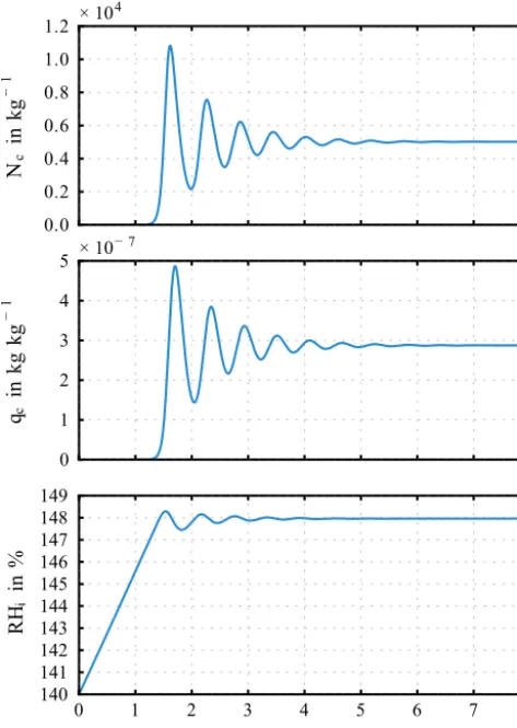
Figure 1.A scenario in state 1 (stable focus regime, damped oscilla-tion) atw=0.01 m s−1andT =220 K. The continuous nucleation as well as similar timescales of nucleation, growth and sedimen-tation leads to a damped oscillation with an equilibrium state for
t >7 h. In phase space, the asymptotic stability is more obvious (see Fig. 5).
– State 1:At rather high temperatures and slow vertical velocities, the three competing microphysical processes (nucleation, growth, sedimentation) are relatively slow and act on similar timescales, so none of them is dom-inant. In particular, nucleation rates are rather small in these cases; therefore, only few ice crystals are formed initially, which grow and also sediment quite slowly. The three processes are more or less in balance, result-ing in a damped oscillation in all three variables, Nc, qc, RHi, asymptotically reaching an equilibrium state, as shown in Fig. 1. Note that, in this state, nucleation is always present, as strong supersaturation with rela-tive humidity close to the nucleation threshold persists at all times and thus the nucleation rates are high enough to produce considerable amounts of ice crystals con-tinuously. This results in smooth oscillations instead of sharp nucleation events, as usually expected (see e.g. Kärcher and Lohmann, 2002). If the air parcel is not
dis-turbed and the vertical updraught remains unchanged in the long-term evolution, the cloud persists and has con-stant ice crystal mass and number concentrations. The cloud in the steady state typically contains low crystal concentrations. The equilibrium state remains at high supersaturations; i.e. the cloud stays far away from ther-modynamic equilibrium.
– State 2: When increasing w or decreasing T, re-spectively, to a certain level, oscillations in variables Nc, qc,RHi are no longer damped (see Fig. 2) and no asymptotic equilibrium can be observed (e.g. a point in phase space). Instead, we obtain pulse-like nucleation with distinct nucleation events followed by phases with almost vanishing nucleation rates at low relative hu-midities. The amplitude of the oscillation is very large in all variables; due to sedimentation, ice particle con-centration is reduced to a small fraction of the maxi-mum value once in a period. At colder temperatures and faster vertical velocities, the nucleation rates are much higher, so nucleation is the dominant process in the beginning, leading to pulse nucleation events. Af-ter a while, ice crystal growth becomes dominant and when the crystals have become large, sedimentation sets in and crystal numbers decrease rapidly. Finally, the cy-cle starts over. In this case, the nucy-cleation events are clearly separated, as opposed to the first case. For the time evolution we find that in the beginning, the ampli-tudes in the three variables decrease slightly from one event to the next, but after a while, the amplitude stays constant. Therefore, it seems that the system asymptot-ically approaches a limit cycle (one-dimensional attrac-tor). This kind of scenario was also observed in former studies (e.g. Spichtinger and Cziczo, 2010; Kay et al., 2006) but not in a long-term behaviour.
Obviously, we find two qualitatively different states in the numerical solution of the model, depending on parametersw andT, respectively. Next, we investigate the model by means of qualitative theory of dynamical systems.
3.2 Qualitative behaviour of the model
0.0 0.2 0.4 0.6 0.8 1.0
Nc
in
kg
−
1
× 105
0.0 0.2 0.4 0.6 0.8 1.0
qc
in
kg
kg
−
1
× 10− 6
0 1 2 3 4 5 6 7 8
Time in h 140
142 144 146 148 150 152 154
RH
i
in
%
Figure 2. A scenario in state 2 (limit cycle regime) is shown at
w=0.02 m s−1andT =210 K. Nucleation events occur as pulses; thus, an undamped oscillation evolves, which describes a limit cycle in phase space (see Fig. 6).
constitute external sinks for cloud variables. Qualitatively, the external sources of water initiate particle generation by nucleation; diffusional growth terms transform water vapour mass into cloud mass until the mass is lost by the external sinks of sedimentation. The model does not fulfil mass con-servation due to sources of water vapour and sinks of cloud mass. Because of the external sinks due to sedimentation the system experiences dissipation. Therefore, the system can be seen as an externally forced dissipative system with non-linear right-hand side.
For a first analysis of the system we compute the diver-gence of the system (i.e. the trace of the JacobianDF): ∇ ·F = −h(b(1−δ)+c(1+δ))Nc−δqcδ+f N1−αi
c qcαi i
+e·w+dαi(RHi−100 %)N1−αi
c qαi
−1 c = −(b(1−δ)+c(1+δ))mδ+f Ncmαi
+e·w+dαi(RHi−100 %)mαi−1 (27)
using the mean mass m=qc/Nc for cloudy states. For clear air (Nc=qc=0), we obtain∇ ·F=e·w >0, hence the system is expanding in phase space. For cloudy air (m >0) there is competition between different terms determining the sign of∇ ·F. Sedimentation and change of relative humid-ity due to diffusional growth are sinks (i.e. negative sign in Eq. 27), while the external source term always has a posi-tive sign. Diffusional growth of ice particles can change its sign depending on the thermodynamic state. Since we always investigate a situation withw >0, the system stays in a su-persaturated state (RHi−100 %>0); therefore, the last term in Eq. (27) is positive.
The balance of terms in Eq. (27), i.e. the sign of∇ ·F for cloudy air, is crucially determined by the mean mass of the cloud. Note that for both exponents we have 0< αi< δ <1, and thus −1< αi−1<0. For large ice crystal mass, the terms of formmδ will dominate, leading to a negative sign of ∇ ·F and to contraction of the system, mainly due to sedimentation of ice crystals. This is especially the case at higher temperatures, since then diffusional growth is faster and mean massesmtend to larger values. In such cases, the system tends to state 1.
For very small ice crystals, the term includingmαi−1will
dominate leading to a positive sign of∇ ·F. For instance, at nucleation events, the ice crystal mass becomes very small; thus, in this situation the system tends to expand explosively (∇ ·F >0). The same is true if almost all particles have fallen out and only small ice crystals are contained in the air parcel. These scenarios are more prevalent at state 2, i.e. at lower temperatures and higher upward velocities.
3.3 Linear stability of the system
In a first step, the autonomous dynamical system Eq. (25) can be characterised by its equilibrium statesx0, i.e. the points in
phase space whereF(x0)=0. The equilibrium states of this
system cannot be determined analytically, due to strong non-linearities. We determine the roots of the right-hand side of system (25) numerically. First, we observe that the mass rate of nucleation dqc
dt
nucleation=a·m0·J (RHi, T )is negligible compared to other mass rates in the system and can be omit-ted for simplification. This leads to a new systemx˙=Fe(x). After settingeF(x)=0, the three resulting equations can be combined to a single equation for RHias follows:
a·J (RHi, T )=
e·w·b f ·
d
c
δ+δ−α1−αi
i
·RHi·(RHi−100 %)
1
0.00 0.01 0.02 0.03 0.04 0.05 w in m s−1
−0.00150
−0.00125
−0.00100
−0.00075
−0.00050
−0.00025 0.00000 0.00025
Real
part
of
complex
eigen
values
Re(
λ1
/
2
)
190 K 200 K 210 K 220 K 230 K
0.00 0.01 0.02 0.03 0.04 0.05 w in m s−1
0.000 0.001 0.002 0.003 0.004 0.005 0.006 0.007 0.008
Imaginary
part
of
complex
eigen
values
|
Im(
λ1
/
2
)
|
190 K 200 K 210 K
220 K 230 K (a)
(b)
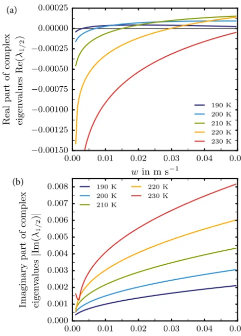
Figure 3.Real (upper panel) and imaginary part (lower panel) of the complex eigenvaluesλ1,2of the JacobianDF|x0at the equilibrium pointx0.
side is strictly monotonic decreasing. Therefore, there ex-ists a unique equilibrium point, x0, in the relevant domain
of the phase space (RHi>100 %,Nc>0,qc>0). The roots of Eq. (28) are determined numerically for the relevant do-main in the parameter space, i.e. 0< w≤0.05 m s−1 and 190≤T ≤235 K.
In order to examine the qualitative behaviour of the solu-tion in a neighbourhood of the equilibrium state, the ODE system is linearised about the equilibrium statex0:
˙
x=F(x0)+DFx
0(x
−x0)+O(|x−x0|2), (29) whereDF|x
0 is the Jacobian ofF evaluated atx0. Note that F(x0)=0 by definition. The three eigenvalues of the
Jaco-bian,λ1, λ2, λ3, determine the quality of the equilibrium state (Verhulst, 1996, chap. 3). The eigenvalues must be deter-mined numerically for the relevant parameter valueswand T. The Jacobian of the system has two complex conjugate eigenvalues,λ1,2∈C, whose real part can be positive or
neg-ative, depending on the parameters,w andT. In Fig. 3 the values of the real partRe(λ1,2)and the absolute value of the
0.00 0.01 0.02 0.03 0.04 0.05 w in m s−1
−0.009
−0.008
−0.007
−0.006
−0.005
−0.004
−0.003
−0.002
−0.001
0.000
Real
eigen
value
λ3
190 K 200 K 210 K
220 K 230 K
Figure 4.Real eigenvalueλ3of the JacobianDF|x0 at the equilib-rium pointx0.
imaginary part|Im(λ1,2)| are shown. The third eigenvalue, λ3∈R, is always negative – values are shown in Fig. 4.
Complex eigenvalues of the linearised system indicate os-cillatory behaviour, which is prevalent in all simulations. As can be seen in Fig. 3, the real part of the complex eigenvalues λ1,2can change its sign depending on parameterswandT.
For negative values of the real part (Re(λ1,2) <0) the equilibrium statex0is stable; i.e. solutions of the ODE (29) starting in a neighbourhood of this point approach this point asymptotically (Verhulst, 1996, Chapter 2). Thus, this equi-librium point can be characterised as stable focus (e.g. Ver-hulst, 1996; Argyris et al., 2010). According to the Poincaré– Lyapunov theorem (Verhulst, 1996, theorem 7.1), an asymp-totically stable linearised system also ensures asymptotic sta-bility of the full nonlinear system Eq. (25). Therefore,x0is
asymptotically stable for the nonlinear system Eq. (25) and constitutes a stable focus. Since there is a unique equilibrium state, all trajectories in phase space tend to this point asymp-totically.
In this case the equilibrium point (stable focus) corre-sponds to state 1 in the numerical simulations. Solutions of the system Eq. (25) experience damped oscillations until they asymptotically approach the stable focus in phase space. The imaginary part of the complex eigenvalues determines the os-cillation period. Figure 5 shows the trajectory of a solution of the system Eq. (25) in the three-dimensional phase space, spiralling towards the equilibrium point.
Nc in kg
− 1 × 10
4
0.0 0.2
0.40.60.8 1.0 1.2
qc in kg kg− 1 × 10− 7
0 1 2 3 4 5 RH
i
in
%
140 141 142 143 144 145 146 147 148 149
Figure 5.Stable focus for state 1 atT =220 K,w=0.01 m s−1: or-bit in phase space approaching the equilibrium state asymptotically.
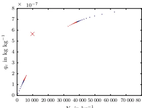
applicable. Numerical integration shows undamped oscilla-tions for soluoscilla-tions that do not start in the equilibrium point; this behaviour points to the possibility of a limit cycle (one-dimensional attractor). The transition from a stable equilib-rium point to limit cycle is a so-called Hopf bifurcation (Ver-hulst, 1996) and is associated with a transition from two con-jugate complex eigenvalues with negative real part to two conjugate complex eigenvalues with positive real part, via two purely imaginary eigenvalues. For a vanishing real part ofλ1,2, the Hopf bifurcation occurs. The existence of a limit cycle cannot be shown analytically for this system; however, we can determine the limit cycle numerically. For starting our calculation close to the limit cycle, we compute the Poincaré map of the system (Argyris et al., 2010; Verhulst, 1996). We choose a two-dimensional plane6in phase space, which is transverse to the trajectory of the solution of Eq. (26);6 is called a Poincaré section. The sequence of points in phase space where the trajectory crosses6 converges numerically to the point on the limit cycle that is in6. Once we find one such point on the limit cycle, we can use it as the initial con-dition in Eq. (26) to compute the complete limit cycle. An example of a Poincaré section for determining the respective limit cycle is shown in Appendix C (Fig. C1). The limit cycle itself constitutes a one-dimensional stable attractor, i.e. solu-tions starting outside of the limit cycle approach the limit cy-cle asymptotically. Figure 6 shows the trajectory of a solution of the system Eq. (25) in the three-dimensional phase space, approaching the limit cycle, which forms a warped circle in phase space.
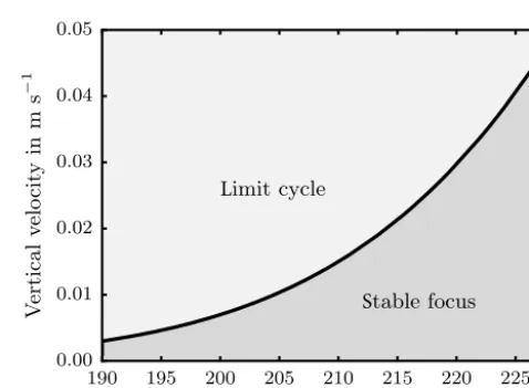
The transition between the two general states of the system (stable point attractor vs. limit cycle) can be represented in a bifurcation diagram of thew–T space (Fig. 7). The bifurca-tion point is a funcbifurca-tion of bothwandT. The different states are separated by points with vanishing real part of eigenval-ues λ1,2, indicated by the thick black line. The bifurcation points were obtained numerically.
Nc in kg − 1 × 10
5
0.0 0.2
0.4 0.6
0.8 1.0 qc
in kg kg− 1
× 10− 6
0.0 0.2 0.4 0.6 0.8 1.0
RH
i
in %
140 142 144 146 148 150 152 154
Figure 6.Limit cycle for state 2: orbit in phase space atT =210 K,
w=0.02 m s−1. Note that the solution starts “outside” of the limit cycle and approaches the limit cycle attractor asymptotically.
190 195 200 205 210 215 220 225
Temperature in K
0.00 0.01 0.02 0.03 0.04 0.05
V
ertical
v
elo
cit
y
in
m
s
−
1
Stablefocus
Limitcycle
Figure 7.Bifurcation diagram for stable focus (state 1) and limit cycle (state 2) regimes in thew–T space. The thick line indicates the location of the Hopf bifurcation.
3.4 Quantitative overview
After discussing the different states of the system qualita-tively, we now give an overview of the quantitative cloud properties and relative humidity for the stable focus and the limit cycle, respectively.
In the stable focus regime, i.e.state 1of the system, the equilibrium state corresponds to the properties of the finally persisting cloud. Hence, in this parameter regime, we de-scribe the properties of the modelled cloud by the values of the system variables at the equilibrium point (stable focus). For the limit cycle regime, i.e.state 2of the system, the un-stable equilibrium pointx0 does not describe the changing
10− 3 10− 2 10− 1
w in m s− 1
102
103
104
105
106
Nc
in
kg
−
1
T = 190 K
T = 200 K
T = 210 K
T = 220 K
T = 230 K
10− 3 10− 2 10− 1
w in m s− 1
10− 9
10− 8
10− 7
10− 6
10− 5
qc
in
kg
kg
−
1
T = 190 K
T = 200 K
T = 210 K
T = 220 K
T = 230 K
(a)
(b)
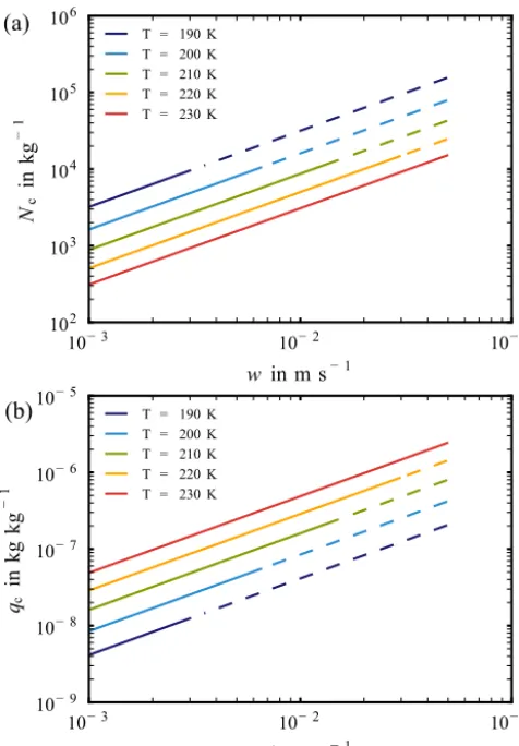
Figure 8.Ice particle number concentrationNc(upper panel) and
ice particle mass concentrationqc(lower panel) at the equilibrium
statex0as a function of vertical velocity for different temperatures.
Solid lines indicate parameter combinations (w,T) in the stable focus regime (state 1); dashed lines represent the limit cycle regime (state 2), i.e. at the unstable focusx0.
revealing measure for the cloud properties in this regime is a probability density of the values the variables take along the limit cycle, or at least median, maximum and minimum values.
Figure 8 shows ice crystal mass and number concentra-tions, respectively, at the equilibrium state,x0, as a function
of vertical velocity (qc(w),Nc(w)) for different temperature regimes. The solid lines in both panels correspond to state 1 (stable focus, damped oscillations), whereas the dashed lines indicate the values at the equilibrium point,x0, for state
2 (limit cycle regime, undamped oscillations); note that for state 2, the equilibrium pointx0is an unstable focus.
Ice crystal number concentrations at the equilibrium point
x0take values in the range 3×10²kg−1≤Nc≤2×10⁵kg−1 (Fig. 8, top), which corresponds to ice crystal number den-sities of 0.1 L−1≤nc≤110 L−1. Ice crystal mass concen-tration ranges between 4×10⁻⁹≤qc≤3×10⁻⁶kg kg−1
(Fig. 8, bottom). This corresponds to an ice water content of 2.2×10⁻⁹≤IWC≤1.4×10⁻⁶kg m−3.
As expected from theory (e.g. Kärcher and Lohmann, 2002) and from former numerical investigations (e.g. Spichtinger and Gierens, 2009), the ice crystal number con-centrations display a strong increase with rising vertical ve-locity. Due to increased crystal growth rates at higher temper-atures,Ncdecreases with risingT. In the double-logarithmic representation in Fig. 8, the number concentrationsNc(w)at the equilibrium pointx0appear as straight lines. For
differ-ent temperature regimes, there seems to be a constant shift between the curvesNc(w), leading to parallel lines in the double-logarithmic representation.
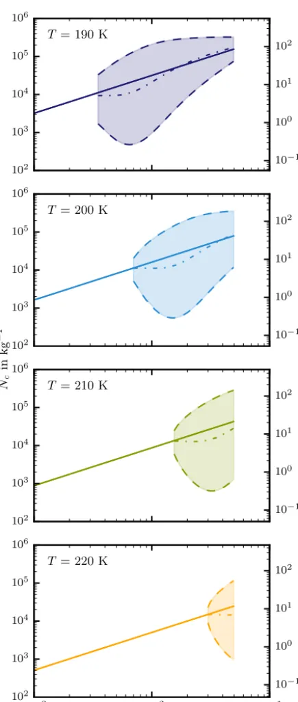
For the limit cycle regime (state 2), we can still derive the values of mass and number concentrations at the equi-librium statex0. However, since this point is an unstable fo-cus, another representation is needed to describe the range of ice crystal concentrations. As indicated in Figs. 7 and 8, the limit cycle behaviour occurs for temperaturesT <230 K for the investigated updraught regime 0≤w≤0.05 m s−1. In Fig. 9 we present maximum and minimum values (dashed lines) and median values (dot-dashed lines) for ice crystal number concentrations in the limit cycle regime for temper-aturesT =190,200,210,220 K. In addition, the ice crystal number concentration at the unstable focus,x0, is displayed (solid lines). We observe a large variation in the number con-centrations of up to two orders of magnitude relative to the median. This behaviour is reasonable since sedimentation re-duces the amount of ice crystals in a dominant manner, while new ice crystals are formed by nucleation in a pulsating way. The absolute values are in the range 0.2≤ρNc≤200 L−1.
The mass concentration of the ice crystals is largely deter-mined by the efficiency of diffusional growth. As indicated in the model description (Sect. 2), this term depends on tem-perature and also on number concentration, leading again to a power law relationship as represented in Fig. 8 (bottom) and to a constant shift between the different temperatures, represented as parallel lines.
For the stable focus regime, we can directly investigate the mean mass of the ice crystals,m=qc/Nc, atx0, which is
dis-played in Fig. 10. The variation ofmat the equilibrium state
x0 due to the vertical velocity is marginal, as indicated in
the figure. Thus, we can assume thatmcan be approximated by a function of temperature. The mean mass atx0 ranges
102
103
104
105
106
T = 190 K
102
103
104
105
106
T = 200 K
102
103
104
105
106
T = 210 K
10−3 10−2 10−1
102
103
104
105
106
T = 220 K
10−1
100
101
102
10−1
100
101
102
10−1
100
101
102
10−1
100
101
102
Nc
in
kg
−
1
win m s−1
nc
in
L
−
1
Figure 9.Ice crystal number concentrations for different temper-ature scenarios (T =190,200,210,220 K). The solid line repre-sents values at the equilibrium statex0(stable or unstable focus). For the limit cycle regime the range of ice crystal number concen-trations is indicated by the shaded area bounded by minimum and maximum values for the updraught range 0.001≤w≤0.05 m s−1; the median is indicated by the dot-dashed line.
190 195 200 205 210 215 220 225 230
Temperature in K
10− 14
10− 13
10− 12 10− 11
10− 10
10− 9
Mean
crystal
mass
in
kg
5 20
10 50 100 150
Mean
crysta
l
size
in
µ
m
Figure 10.Mean ice crystal massmas a function of temperature. For the equilibrium state x0, values of mdepends only slightly on the vertical velocity, the curve covers the area that corresponds to vertical velocities 0.001 m s−1≤w≤0.05 m s−1. Additionally, box-and-whisker plots indicate median, 25th/75th percentiles, and minimum/maximum values, respectively, for the limit cycle regime.
0.00 0.01 0.02 0.03 0.04 0.05 w in m s−1
0 5000 10000 15000 20000 25000 30000
P
erio
d
in
s
190 K 200 K 210 K 220 K 230 K
Figure 11.Oscillation periods for the stable focus regime at x0
(solid lines), and for the limit cycle regime (dashed lines). For the stable focus regime, the periods are obtained from the imaginary part of the complex eigenvalues; for the limit cycle regime, the pe-riods are calculated using the Poincaré map.
As indicated in Sect. 3.3, the imaginary part of the com-plex eigenvaluesλ1,2 determines the period of the oscilla-tions in state 1 (stable focus regime) near the equilibrium pointx0. In Fig. 11 the periodτ =Im(λ2π
1,2) as calculated from
the imaginary part is shown for the stable focus (solid lines; colours indicate different temperature regimes). For the un-stable focus, the imaginary part of the eigenvalues is not meaningful, as the limit cycle is not within the linear regime ofx0. Instead, the periods of the limit cycle is shown (dashed
3.5 Comparison with observations
For comparison with observations we first consider in-situ measurements of ice crystals in subvisible cirrus clouds. Since it is very difficult to measure low number concen-trations, only few measurement studies are available. We compare our results with measurements by Kübbeler et al. (2011), Lawson et al. (2008) and Davis et al. (2010). Our model results lead to ice crystal number concentrations in the range 0.1 L−1≤ρNc≤200 L−1and mean ice crystal sizes in the range∼16 µm≤L≤134 µm. Note that the variation in number concentrations span over 3 orders of magnitude and the variation in mean sizes is still within 2 orders of magnitude. These simulated values agree quite well with the measurements. Kübbeler et al. (2011) observed quite high number concentrations of the order of ∼100 L−1for small ice crystals (L∼10 µm) but quite low number concentra-tions 0.1≤ρNc≤10 L−1 for large ice crystals (equivalent radiusr >50 µm). Lawson et al. (2008) reported ice crystal number concentrations in the range 22.5≤ρNc≤188.8 L−1 with mean value and standard deviation 66±30.8 L−1 for ice crystals in the size range 1≤L≤200 µm. Finally, Davis et al. (2010) reported very low ice crystal number concentra-tions with a mean value of 2 L−1 and mean sizes of 14 µm during the tropical measurement campaign TC4. However, in their study values from former measurement campaigns are reported to be in the range 10≤ρNc≤100 L−1and for effective radii 10≤r≤20 µm.
In a second step we expand our comparison to observa-tions from remote sensing. Since SVCs are optically very thin, we investigate the extinction coefficient for the visible part of the spectrum. For comparing our results with mea-surements, we calculate the extinctionβ in the solar range using parameterisations by Fu and Liou (1993):
β=IWC·
a+ b De
, (30)
where IWC=qc·ρ denotes ice water content in g m−3and De in µm is the generalised size. Constants are given by a= −6.656×10⁻³m2g−1 and b=3.686 µm m2g−1. As a useful approximation we set De=L, where the quantity L is calculated from the mean massmusing the mass–length relationL=Cimαi, as indicated in Appendix A. In Fig. 12
the values forβare shown for different temperature regimes as calculated for the mean values at the (stable and unstable) focus (equilibrium point). Note that there is only marginal difference in the values for different temperatures. The val-ues are within the interval 10−4≤β≤0.02 km−1.
Seifert et al. (2007) report mean values for extinctions of SVCs in the range 0.015≤β≤0.02 km−1 with stan-dard deviations σ∼0.005–0.009 km−1 (see their Table 3). Our results are in the same order of magnitude or even smaller for slow vertical updraughts. Davis et al. (2010) report much smaller values of extinction scattered in the range 0< β <0.01 with a mean value ofβ∼0.001 km−1.
0.01 0.02 0.03 0.04 0.05 w in m s−1
10−4
10−3
10−2
βext
in
km
−
1
T= 190 K T= 200 K T= 210 K T= 220 K T= 230 K
Figure 12.Extinction coefficient atx0for different temperatures in the stable focus state 1 (solid lines) and the limit cycle state 2 (dashed lines).
These SVCs were measured in the tropics at high altitudes (z∼16 km), i.e. at low temperaturesT <195 K, where slow large-scale updraughts due to Kelvin waves of the order of w <0.01 m s−1dominate (Immler et al., 2008b). This is con-sistent with our results; see Fig. 12.
Overall, we can state that regarding the high spread in the measurements the results from our reduced model agree quite well with in situ measurements.
3.6 Comparison with other models
For comparison with a more detailed model, we carried out simulations with the box model described by Spichtinger and Gierens (2009) and Spichtinger and Cziczo (2010). This model includes more sophisticated treatment of microphysi-cal processes, although it is also a two-moment bulk model. It allows a change in the shape of ice crystals from almost spherical droxtals to columns. Homogeneous nucleation is treated in detail, including deliquescence of sulphuric acid and integration over the full size distribution of solution droplets. For diffusional growth, kinetic and ventilation ef-fects are included. Finally, temperature and pressure changes due to vertical upward motions and latent heat release is added to the air parcel’s temperature.
0.0 0.2 0.4 0.6 0.8 1.0 1.2
Nc
in
kg
−
1
×104
0 1 2 3 4 5
qc
in
kg
kg
−
1
×10−7
0 1 2 3 4 5 6 7 8
Time in h
140 142 144 146 148 150 152 154
RH
i
in
%
Reducedmodel,thisstudy Spichtinger and Gierens, 2009
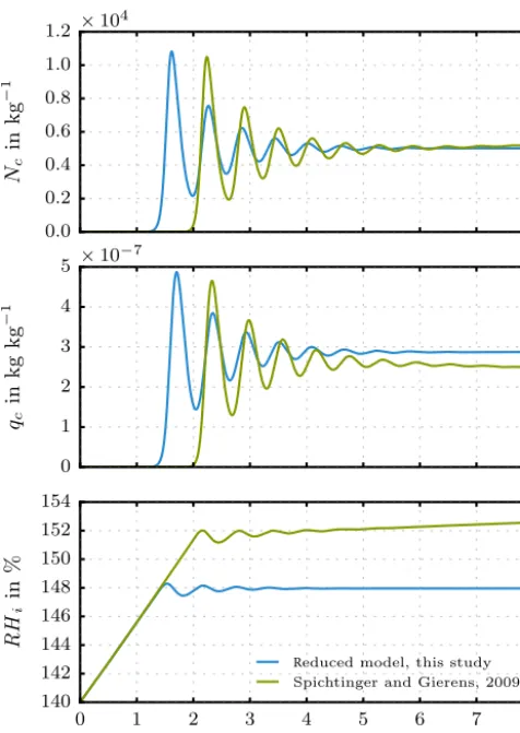
Figure 13.Stable focus case (state 1): comparison between reduced model (this study) and the complex box model by Spichtinger and Gierens (2009). Updraughtw=0.01 m s−1, temperature in the re-duced model and start temperature of the complex model is T= 220 K.
We can again identify regimes in theT–wparameter space representing the known two different states, i.e. damped os-cillations (stable focus regime, state 1) and limit cycle be-haviour (state 2). In Fig. 13 the case of damped oscillation is shown in both model simulations. Here, initial temperature of T =220 K is used with a vertical velocity ofw=0.01 m s−1. Green lines indicate the evolution in the complex model sim-ulation, whereas blue lines represent the evolution in the re-duced model. For the variables number and mass concentra-tion, both models produce almost the same values. The onset of ice nucleation is shifted between the two models due to differently detailed representation of ice nucleation in both models. This leads to the difference in relative humidity val-ues. Qualitatively, the models agree very well – the oscil-lation periods and the magnitudes of the damping are very similar.
For the complex model simulations the environmental conditions change; i.e. temperature and pressure are decreas-ing due to adiabatic expansion. Thus, no steady state can
0.0 0.2 0.4 0.6 0.8 1.0
Nc
in
kg
−
1
×105
0.0 0.2 0.4 0.6 0.8 1.0
qc
in
kg
kg
−
1
×10−6
0 1 2 3 4 5 6 7 8
Time in h
140 142 144 146 148 150 152 154 156 158
RH
i
in
%
Reducedmodel,thisstudy Spichtinger and Gierens, 2009
Figure 14.Limit cycle case (state 2): comparison between reduced model (this study) and the complex box model by Spichtinger and Gierens (2009). Updraughtw=0.02 m s−1, temperature in the re-duced model and start temperature of the complex model isT = 210 K.
be reached. The values for ice crystal number concentra-tions and relative humidity are slightly rising with time in the quasi-steady state at the end of the simulation. Ice crystal mass concentration is slightly decreasing.
In Fig. 14, a case of limit cycle behaviour is shown. As in Fig. 13, green lines indicate the complex model simulations and the reduced model results are represented by blue lines, respectively. The initial conditions for both models are given byT =210 K andw=0.02 m s−1. Again, we find very good agreement in the cloud variablesNc,qcbetween both model simulations. Qualitatively they also agree very well in terms of the periods of the oscillations.
evolu-tion initially follows the damped oscillaevolu-tions as expected from the bifurcation diagram of the reduced model. How-ever, the temperature change leads to a (horizontal) path in the phase diagram (Fig. 7) and at some stage the boundary between the two states is crossed, and from then on, the sys-tem will perform undamped oscillations. Indeed, we observe this transition in the complex model simulations. An exam-ple for this situation is given in Fig. 15, with initial conditions T =225 K andw=0.035 m s−1. Note that in the limit cycle regime the properties of the theoretically expected limit cycle also change with decreasingT. This results in increasing am-plitudes of the oscillations in Nc,qc, RHi and in increasing periods. Thus, we can conclude that for realistic simulations including changes in environmental conditions there could be transitions between the theoretically determined states. How-ever, the behaviour of the actual states can still be explained by the phase diagram as obtained from our analytical consid-erations.
We also compare our results with the analytical model by Kärcher (2002), which includes a more sophisticated rep-resentation of nucleation and growth. The relevant equa-tions are treated using typical timescales and approxima-tion of the occurring integrals. Comparison with results by Kärcher (2002) shows good agreement as well. Actually, in our investigations with the reduced model we found low ice crystal number concentrations similar to results by Kärcher (2002); the dependence of number concentrations onwand T also agrees very well with analytical considerations by Kärcher (2002). However, our approach goes beyond the re-sults by Kärcher (2002) since we allow for sedimentation of ice crystals. This additional process leads to the oscillatory behaviour in both states, whereas in the study by Kärcher (2002) a quasi-steady state at ice saturation is reached soon. Especially the continuous nucleation in the state 1 scenario (stable focus, damped oscillation) is only possible if we al-low for sedimentation of ice crystals. Otherwise, the nucle-ation event would stop after depositional growth has reduced the supersaturation such that nucleation rates become negli-gible. Thus, our scenarios might be more realistic, although values of mass and number concentrations in both studies are very similar.
4 Conclusions
In this study we have developed a reduced model for describ-ing subvisible cirrus clouds formed by homogeneous nucle-ation in the tropopause region. The model consists of a set of autonomous ordinary differential equations for the variables ice crystal mass and number concentration, and relative hu-midity with respect to ice. It contains the relevant cloud pro-cesses ice nucleation, diffusional growth and sedimentation. The model can be viewed as an externally forced dissipative system. The model is integrated numerically and also inves-tigated using (linear) theory of dynamical systems.
0 1 2 3 4 5 6 7 8
Nc
in
kg
−
1
× 104
0.0 0.5 1.0 1.5 2.0 2.5 3.0
qc
in
kg
kg
−
1
× 10− 6
0 2 4 6 8 10 12
Time in h
140 142 144 146 148 150 152 154 156 158
RH
i
in
%
220 K 215 K 210 K
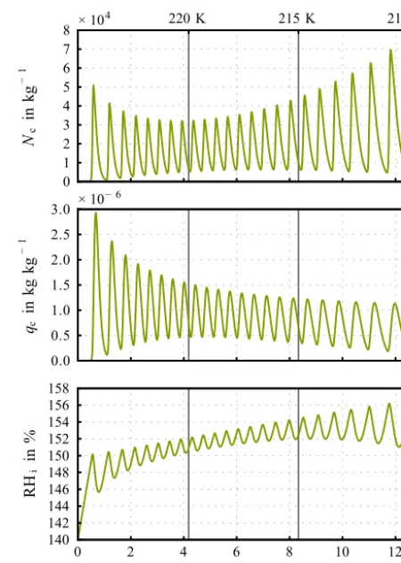
Figure 15.Transition between stable focus regime (state 1) and limit cycle regime (state 2): simulation with the complex model by Spichtinger and Gierens (2009) forw=0.035 m s−1and start tem-perature:T =225 K. During the first 2 h of the simulation, the sink property can be clearly seen. After reaching temperatures of about
T∼220 K, the regime changes from state 1 (stable focus) to state 2 (limit cycle); see also phase diagram in Fig. 7. After this transition, the amplitudes of number concentrations and relative humidity with respect to ice increase and at the end of the simulation also a shift in the oscillation period can be seen. Increase in amplitude and shift in oscillation period are due to changes of the limit cycle properties for decreasing temperature (see e.g. Fig. 11)
Integration and theoretical analysis show that the system contains two different states, a stable focus state and a limit cycle state. The states depend on the environmental parame-ters vertical updraught,w, and temperature,T. The transition between the states can be described as Hopf bifurcation. Both states show oscillatory behaviour, either damped (stable fo-cus) or basically undamped (limit cycle).
vertical velocity; thus, we can approximate the mean mass as a function of temperature.
Comparisons with a more detailed box model by Spichtinger and Gierens (2009) show very good agreement. The qualitative behaviour as determined for the reduced model can also be found for the complex model simulations. Also, in terms of quantitative results both models agree quite well. Former analytical investigations by Kärcher (2002) show good agreement with our reduced model, too. However, since we include sedimentation in our model, our results go clearly beyond the former investigations; the long-term be-haviour is different, since the inclusion of sedimentation cru-cially leads to the bifurcation, depending on environmental conditions.
Since there are only few in situ measurements of subvisi-ble cirrus availasubvisi-ble, it is quite difficult to carry out solid com-parisons. However, we try to compare with measurements as described by Kübbeler et al. (2011), Lawson et al. (2008), and Davis et al. (2010) and find good agreement with our model results. Also, the extinction coefficient as calculated from model results agrees very well with observations ob-tained with remote sensing techniques (Seifert et al., 2007; Davis et al., 2010).
The major qualitative results can be summarised as fol-lows:
– Homogeneous freezing of aqueous solution droplets at low temperatures (T <235 K) is a possible pathway for the formation of subvisible cirrus clouds at low verti-cal updraughts. Thus, the question about the dominance of formation mechanisms for these thin clouds remains open (homogeneous vs. heterogeneous nucleation). – In unperturbed weak large-scale updraughts subvisible
cirrus clouds can exist in two different qualitative states, reaching either a stable equilibrium point (stable focus) in the long-term behaviour or experiencing oscillation behaviour in a limit cycle scenario. The state depends on external parameters as large-scale updraught and tem-perature, respectively.
– The cloud particle properties in the long-term behaviour are very similar for both states. Therefore, we cannot decide from values of mass and/or number concentra-tions in a certain range in which state the cloud might be. Even if we had more measurements, we probably would not be able to decide between the two states just using the Eulerian measurements without a Lagrangian point of view.
We might derive a minimal model for SVCs from the bi-furcation diagram in the following way. If we assume that SVCs are well approximated by their attractors, we could express cloud variables and relative humidity by a simple damped harmonic oscillator of the form
¨
x+κx˙+ωx=0, (31)
withx∈ {Nc, qc,RHi}and parametersκ=κ(w, T )andω= ω(w, T ), respectively.κ describes damping, whereasω rep-resents oscillation frequency.κ, ω can be determined using eigenvaluesλifor damping and oscillations in the stable fo-cus case (κ6=0). For the limit cycle case (κ=0), periods as obtained from the Poincaré section (see Fig. 11) can be used for describingω. Such a minimal model could be used for representing SVCs in large-scale models and can be seen as a prototype for new-generation cloud parameterisations. These models describe the structure of clouds in terms of cloud variables and environmental conditions. They could be used for describing such structures embedded into a coarse-grid model. However, further research in this direction is neces-sary in order to proceed from pure model prototypes to useful cloud parameterisations.
Finally, we can state that we could develop a meaningful reduced model for describing the main features of subvisible cirrus clouds. Former investigations using box models indi-cated that there might be different regimes in the behaviour of the clouds for longer simulation times. For instance, in studies by Kay et al. (2006) and Spichtinger and Cziczo (2010) oscillatory behaviours as well as asymptotic stability could be seen. However, only a detailed mathematical analy-sis could show that there is a bifurcation in the long-term be-haviour and that it depends mostly on environmental param-eters such as updraught velocity and temperature. This anal-ysis was only possible since we developed a reduced model, which is close enough to complex models but is also simple enough for mathematical analysis.
The observed Hopf bifurcation as a transition between two different states shows that clouds might exhibit inherent structures, which are crucially determined by the microphys-ical cloud processes themselves in addition to environmental conditions. Similar structure formation was already seen in analytical cloud models for liquid and mixed-phase clouds as developed by Wacker (1992, 1995, 2006) or Hauf (1993). Investigation and analysis of the microphysical processes in terms of sets of ordinary differential equations are a first but urgently necessary step in order to investigate structure formation inside clouds. Once we understand the possible structures in clouds as determined by microphysics, we can continue to further investigate structure formation as driven by spatial diffusion processes, mixing and others, leading to spatial structures of clouds. A first possible approach might be to investigate equations with additional spatial diffusion terms regarding possible Turing instabilities (Turing, 1952). However, further research is necessary in order to investigate structure formation of ice clouds.
Data availability. The data used in this work are described in
Appendix A: Details of parameterisations A1 Nucleation
Homogeneous nucleation, i.e. the transformation of a solu-tion droplet to an ice crystal, can be seen as a stochastic pro-cess. The transition rateωfor the transformation of a solution droplet of volumeV can be expressed using a volume nucle-ation rateJ, i.e.ω=V·J. The probabilityP (t )for the nu-cleation process of droplets of volumeV fulfils the following differential equation:
dP
dt = −ωP (t ). (A1)
For further details of the general derivation we refer the reader to Koop et al. (1997). Equation (A1) can be gener-alised for size distributions of solution droplets, leading to the formulation of Eq. (7). Koop et al. (2000) provide a pa-rameterisation for the volume nucleation rateJ as a function of1aw:=aw−awi (Koop et al., 2000, Table 1, Eq. 7). Here aw is the water activity of the solution andawi is the water activity of the solution in equilibrium with ice. Note that the freezing characteristics of the droplets do not depend on the chemical composition. By definition the water activity is the ratio psol/pliq of the vapour pressure over a solution,psol, and pure liquid water,pliq. Neglecting the Kelvin effect and assuming that the solution droplets are in equilibrium with the environment (pv=psol), we find that the water activity is proportional to the water activity in equilibrium with ice, which is the ratio of the water vapour pressure over ice and pure liquid water:
aw=psol pliq
= pv pliq
= RHi 100 %
psi pliq
= RHi 100 %a
i
w. (A2)
Bothpsiandpliqonly depend on temperature and are param-eterised according to Murphy and Koop (2005, Eqs. 7 and 10, respectively). Hence,1awis a function of RHiandT, as given by
1aw(T ,RHi)=
RH
i 100 %−1
awi(T )
=
RH
i 100 %−1
p
si pliq
. (A3)
ThereforeJ is also a function of RHiandT. The logarithm of the nucleation rate is parameterised by a third-order poly-nomial in1aw(Koop et al., 2000, Table 1, Eq. 7):
log10J (T ,RHi)= −906.7+85021aw
−26 924(1aw)2+29 180(1aw)3. (A4) A2 Diffusional growth
The “advection velocity”gin the mass space is given by the growth equation for a single ice crystal; this equation has the
following form (see e.g. Stephens, 1983): g(m)=dm
dt =4π CD
∗
vρqv,si
RH
i 100 %−1
fv. (A5) Here,qv,si=ε psi(T )/pdenotes the saturation mixing ratio, the shape of the ice crystal is accounted for by the capacity C (assuming the electrostatic analogy; see e.g. McDonald, 1963; Jeffreys, 1918),Dv∗ is the full diffusion constant in-cluding the kinetic correction for small particles (Lamb and Verlinde, 2011) andfvdenotes the ventilation coefficient.
In this study we make use of the following simplifications: 1. Latent heat release at the crystal surface is neglected and the temperature of the ice particles is assumed to be equal to temperature of ambient air.
2. We neglect kinetic corrections, since we are mostly in-terested in growth of larger crystals. Kinetic corrections are usually important for ice crystal growth in regimes with high concentrations of small crystals. For SVCs we can assume small number concentrations; thus, crystals will grow fast to sizes larger than∼10 µm. Thus, we can assume
D∗v≈Dv=D0
T T0
α
p0 p
, (A6)
with D0=2.11×10⁻⁵m2s−1, T0=273.15 K, p0= 101 325 Pa,α=1.94 (e.g. Pruppacher and Klett, 1997). 3. We neglect correction of ventilation, setting fv=1. Ventilation correction is only relevant for very large crystals, so this is a reasonable assumption, since in SVCs ice crystals are usually smaller than∼200 µm. 4. The shape of ice crystals is assumed to be prolate
spheroids with lengthL and an eccentricityε0, which leads to the following expression (McDonald, 1963): C=L ε
0
log11+−εε00
. (A7)
For the mass–length relation we assume a simple power law L(m)=Cimαi using Ci=1.02 m kg−αi, αi=0.4.
This power law mostly represents the columnar shape of ice crystals, which is assumed for crystals with sizes L >10 µm. The power law was fitted to a more complex description in Spichtinger and Gierens (2009), where a transition between droxtals and columns is formulated and used.
The fraction in Eq. (A7) only depends weakly on the crys-tal mass and can be approximated by a constant mean value of 1/3. This yields
C=1 3Cim