https://doi.org/10.5194/tc-12-3747-2018
© Author(s) 2018. This work is distributed under the Creative Commons Attribution 4.0 License.
The potential of sea ice leads as a predictor for summer
Arctic sea ice extent
Yuanyuan Zhang1,2,4, Xiao Cheng1,2,4, Jiping Liu3, and Fengming Hui1,2,4
1College of Global Change and Earth System Science, and State Key Laboratory of Remote Sensing Science, Beijing Normal University, Beijing 100875, China
2Joint Center for Global Change Studies (JCGCS), Beijing 100875, China
3Department of Atmospheric and Environmental Sciences, University at Albany, State University of New York, Albany, NY 12222, USA
4University Corporation for Polar Research, Beijing 100875, China
Correspondence:Xiao Cheng (xcheng@bnu.edu.cn) Received: 22 May 2018 – Discussion started: 9 July 2018
Revised: 1 October 2018 – Accepted: 31 October 2018 – Published: 30 November 2018
Abstract.The Arctic sea ice extent throughout the melt sea-son is closely associated with initial sea ice state in winter and spring. Sea ice leads are important sites of energy fluxes in the Arctic Ocean, which may play an important role in the evolution of Arctic sea ice. In this study, we examine the po-tential of sea ice leads as a predictor for summer Arctic sea ice extent forecast using a recently developed daily sea ice lead product retrieved from the Moderate-Resolution Imag-ing Spectroradiometer (MODIS). Our results show that July pan-Arctic sea ice extent can be predicted from the area of sea ice leads integrated from midwinter to late spring, with a prediction error of 0.28 million km2 that is smaller than the standard deviation of the observed interannual variability. However, the predictive skills for August and September pan-Arctic sea ice extent are very low. When the area of sea ice leads integrated in the Atlantic and central and west Siberian sector of the Arctic is used, it has a significantly strong rela-tionship (high predictability) with both July and August sea ice extent in the Atlantic and central and west Siberian sec-tor of the Arctic. Thus, the realistic representation of sea ice leads (e.g., the areal coverage) in numerical prediction sys-tems might improve the skill of forecast in the Arctic region.
1 Introduction
Sea ice is an important component of the climate system. In the past few decades, Arctic sea ice has undergone dra-matic change associated with changes in atmospheric and oceanic processes (Comiso et al., 2008; Ding et al., 2017; Liu et al., 2013; Parkinson and Comiso, 2013; Richter-Menge et al., 2016; Stroeve et al., 2007, 2012). Satellite observation shows a decreasing Arctic sea ice extent at an annual rate of about 4.73 % per decade and a faster rate of 13.56 % per decade in September for the period of 1979–2017, calculated using the Arctic sea ice index obtained from the National Snow and Ice Data Center (see Sect. 2 for details of data). The decreasing Arctic sea ice not only affects the local envi-ronment and community, i.e., brings opportunities and chal-lenges to indigenous people (Forbes et al., 2016; Lamers et al., 2016), but also has strong feedback on other components of the climate system, i.e., increases the frequency of abnor-mal weather and climate in the midlatitudes of the North-ern Hemisphere and influences the thermohaline circulation (Budikova, 2009; Levermann et al., 2007; Liu et al., 2012; Vihma, 2014). Hence there is an increasing demand for Arc-tic sea ice prediction at seasonal and longer timescales, es-pecially during the melting season (Eicken, 2013; Stroeve et al., 2014).
regression-type statistical models, trained from historical data and then applied to forecast the near future. To date, statistical models show comparable or slightly higher skill than dynamic models in terms of the prediction of the total Arctic sea ice extent (Blanchard-Wrigglesworth et al., 2015; Stroeve et al., 2014). The evolution of Arctic sea ice ex-tent during summer and fall is closely associated with ini-tial sea ice conditions in winter and spring. The potenini-tial of different sea ice parameters as predictors of Arctic sea ice extent has been explored using empirical statistical models. The results show that some parameters can significantly con-tribute to the improvement in seasonal sea ice forecast skill at different lead times (Holland and Stroeve, 2011; Lindsay et al., 2008). For example, sea ice concentration and surface temperature in spring are introduced into a multiple linear re-gression model to forecast the minimum Arctic sea ice extent (Drobot, 2007; Drobot et al., 2006). Some studies suggested that accurate sea ice thickness can increase forecast skill 2 months ahead (Day et al., 2014; Dirkson et al., 2017). Re-cently, the spring melt pond fraction has been employed to improve the skill of forecasting September sea ice extent (Liu et al., 2015; Schröder et al., 2014). An annual sea ice outlook has solicited prediction of mean September Arctic sea ice extent from the research community since 2008. The result shows that the median sea ice predictions are off by a large margin in 2009, 2012 (record low), 2013, 2014 and 2016 (second record low) (Hamilton and Stroeve, 2016; Stroeve et al., 2014).
Sea ice leads develop as quasi-rectilinear cracks within the ice pack due to sea ice dynamics and warm water upwelling at particular locations. Leads can be kilometers to tens of kilometers long and meters to kilometers wide, which are more prevalent in areas of thin ice (i.e., the marginal ice zone) than in the central Arctic ice pack (Wadhams et al., 1985). Though leads only cover a small proportion of sea ice area, they are important sites of energy fluxes that can cause a large fluctuation of air temperature (Lüpkes et al., 2008). Leads are responsible for about 50 % of a transfer of sensible heat from the Arctic Ocean to the atmosphere during winter (Maykut, 1982). In situ measurements from the Arctic Ice Dynamics Joint Experiment Sea Ice Lead Experiment in 1974 showed that sensible heat and latent fluxes from leads can exceed 400 and 130 W m−2, respectively (Andreas et al., 1979). Sensi-ble heat flux over sea ice leads depends strongly on leads’ width. Narrow leads are over 2 times more efficient in trans-ferring heat than larger ones (Maykut, 1982). When consid-ering the leads’ width influence in the assessment, heat flux can be up to 55 % larger (Marcq and Weiss, 2012). In addi-tional, the albedo of leads is about 0.07 under cloudy con-ditions (Tschudi et al., 2002) in contrast to 0.6–0.9 of sea ice or snow-covered ice (Perovich et al., 2002). As a result, the leads absorb more shortwave radiation. Adversely, sea ice leads that persist throughout the winter are often accom-panied by low-level clouds downwind because of the release
of heat and moisture into the atmosphere, influencing the sur-face energy budget.
While sea ice leads play an important role in the determi-nation of the evolution of Arctic sea ice, their potential role in Arctic sea ice prediction has not been examined. One rea-son is a lack of observations of sea ice leads with sufficient spatial and temporal coverage. This hampers our understand-ing of the variability of sea ice leads in the Arctic Ocean, and their relationship with Arctic sea ice cover (Ivanova et al., 2016; Wernecke and Kaleschke, 2015). Another reason is that sea ice leads constitute an unrepresented process in nu-merical prediction systems and climate models due to their highly nonlinear, small-scale and intermittent characteristics (Spreen et al., 2017; Wang et al., 2016). As a result, poten-tial effects of sea ice leads on Arctic sea ice prediction are not well understood. Given that sea ice leads dominate the atmosphere–sea ice–ocean interface in the aforementioned manner, in this study, we use a recently developed sea ice lead product retrieved from the Moderate-Resolution Imag-ing Spectroradiometer (MODIS) thermal infrared data to ex-amine the potential of sea ice leads as a predictor for summer Arctic sea ice extent forecasts.
2 Data and methods
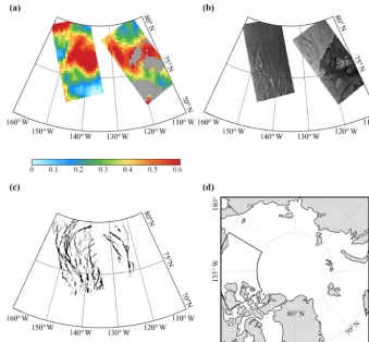
Figure 1. (a)MODIS cloud fraction (%),(b)SAR backscatter coefficient image, and(c)MODIS sea ice leads in the highlighted area (the northern Beaufort Sea) as shown by the box in(d)on 11 April 2015.
In a recent study, Willmes and Heinemann (2015a) pre-sented a non-parameterized global threshold method, which was validated and applied to derive sea ice leads maps from surface temperature anomalies in the Arctic Ocean using the MODIS ice surface temperature product. Daily sea ice lead composites were created. The composite maps indicate the presence of cloud artifacts in the leads’ identification that arise from ambiguities in the MODIS cloud mask. To mit-igate these artifacts, they implemented a fuzzy filter system that employs spatial and temporal object characteristics to distinguish between physical leads and artifacts. This ap-proach advances the potential to retrieve daily leads maps operationally from the MODIS infrared product.
In this study, the pan-Arctic sea ice leads data are obtained from the Data Publisher for Earth & Environment Science (PANGAEA), which is available for the months from Jan-uary to April for the period 2003–2015 (Willmes and Heine-mann, 2015b). The spatial resolution of the daily binary sea ice lead map is about 1.5 km with the omission of 5 % that can reflect sea ice lead variability except the Chukchi Sea (Willmes and Heinemann, 2015a, c) because clear-sky day is less than 15 % in the Chukchi Sea. Cloud contamination is a major issue plaguing the retrieval of the pan-Arctic sea ice leads from the MODIS infrared observation. Here we
com-pare the above MODIS sea ice leads data with the SAR im-ages under cloudy conditions. Compared to MODIS that re-ceives thermal emissions or reflected components, SAR al-lows for penetration through most clouds and precipitation. We calculate backscatter coefficients from the Sentinel-1A Extra-Wide swath HH polarization images using the Sentinel Application Platform and project them on the NSIDC polar-stereographic grid with a spatial resolution of 100 m. Cloudy conditions are determined using the MOD08 Level3 daily cloud fraction product (Hubanks et al., 2018). For example, Fig. 1 shows the MODIS cloud fraction, the SAR backscatter coefficient image, and MODIS sea ice leads in the northern Beaufort Sea on 11 April 2015. Compared to SAR images, the MODIS sea ice lead data can capture the correct spa-tial distribution of sea ice leads under cloudy conditions. The consistence between the MODIS sea ice lead data and the SAR image gives us more confidence in these data.
The daily total area of sea ice leads is computed from the daily binary sea ice leads map, which is projected on the NSIDC polar-stereographic grid with a spatial resolution of 25 km. During the projection, we calculate the number of pixels with detected sea ice leads in a 25 km grid box. The sea ice lead fraction is then defined as the ratio between the number of pixels with detected sea ice leads and the total number of pixels in the 25 km grid box. The total area of sea ice leads is the sum of the product of the sea ice leads fraction and the area of the grid box (625 km2). Here the daily total area of sea ice leads is only calculated when the NSIDC sea ice concentration in the grid box is larger than 15 % (com-monly used as the threshold to define the sea ice edge).
3 Results
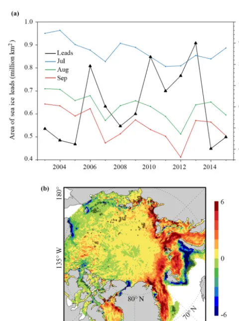
Figure 2 shows the evolution of the daily total area of sea ice leads in the Arctic Ocean from 1 January to 30 April averaged for the period of 2003–2015. Superimposed on large year-to-year variation for each single day as shown by the grey shading in Fig. 2, the climatology of the to-tal sea ice lead area exhibits a gradually decrease from ∼ 0.8 million km2in early January to∼0.5 million km2in late April. As shown in Fig. 3a, overall, there is no significant trend in the total area of sea ice leads averaged for January– April during 2003–2015, although it shows an increasing ten-dency from 2003 to 2013. The year 2013 had the largest area of sea ice leads (0.91 million km2) followed by the small-est area in the year 2014 (0.45 million km2). We also cal-culate the correlation coefficients between July, August and September sea ice extent and the area of sea ice leads av-eraged from January to April during 2003–2015, which are −0.51,−0.30 and−0.23, respectively. It appears that July sea ice extent is more closely related to the area of sea ice leads than August and September. Figure 3b shows the spa-tial distribution of the trend of the sea ice lead area in each in-dividual 25 km grid box. The area of sea ice leads has exhib-ited an increasing trend extending from the Greenland Sea, through the northern Barents Sea, to the Laptev and Kara seas, and a decreasing trend in the southern Barents Sea, be-tween the eastern Siberian Sea and Chukchi Sea, and along the coast of Alaska. In particular, the strong out-of-phase trend between the northern and southern Barents Sea is per-sistent for each individual month. However, most of these trends are not significant at the 95 % confidence level, except the southern Barents Sea.
To investigate the relationship between the area of sea ice leads in the Arctic Ocean from late winter to mid-spring and Arctic sea ice extent during the melting season, we calculate the correlation between the time series of the sea ice lead area averaged for January–April and sea ice extent in July, August and September, respectively, during 2003–2015. It should be noted that when examining correlation between two variables with large trends, two variables might be linked statistically
Figure 2.Time series of the daily area of pan-Arctic sea ice leads from 1 January to 30 April for the period of 2003–2015. The black solid line is the averaged area during 2003–2015 and the grey shad-ing denotes 1 standard deviation of interannual variability.
but be physically independent. Thus, we remove the trend for all time series before calculating the correlation.
Following similar procedures in Liu et al. (2015), we inte-grate the area of sea ice leads in the Arctic Ocean over time and space to generate the sea ice lead time series. Specif-ically, first, we integrate the average area of sea ice leads occurring in each individual 25 km grid point varying from 1 to 2 January, to 3 January, and up through 30 April. Sec-ond, we calculate the correlation coefficient between the de-trended time series of the integrated area of sea ice leads at each grid point and the de-trended time series of the total sea ice extent in July, August and September, respectively. As discussed earlier, in general, more sea ice leads during late winter to mid-spring, even when they refreeze, tend to contain thinner and weaker sea ice that is more susceptible to atmospheric winds (i.e., storm) and air temperature (i.e., warm advection). This may result in less sea ice during the melting season. Thus, more sea ice leads are expected to neg-atively associate with subsequent sea ice extent, so we expect negative correlations between sea ice leads and sea ice extent. Figure 4 shows spatial correlation maps between the area of sea ice leads integrated from 1 January to the day given and the total Arctic sea ice extent in July, August and September, respectively. For July sea ice extent (Fig. 4a– d), some small clusters of significant negative correlations, though scattered, are found in the Arctic Ocean north of ∼75◦N as the area of sea ice leads is integrated for 1 month from 1 to 30 January (black crosses in Fig. 4a). These small clusters become relatively broader as the area of sea ice leads is integrated to the end of February (60 days, Fig. 4b), cover-ing a relatively larger percentage of the central Arctic Ocean as well as much of the western Greenland Sea and northern Barents and Kara seas. By the end of March, extending the integration to 90 days, the area with significant correlations is enlarged remarkably, especially in the Atlantic and central and west Siberian sector of the Arctic (Fig. 4c). Extending the integration to the end of April (120 days), the area with significant correlations has minimal change (Fig. 4d) com-pared to that of Fig. 4c. The spatial distribution of significant correlations for August and September sea ice extent is sim-ilar (Fig. 4e–l).A small cluster of significant negative corre-lations is found in the western Laptev Sea as the area of sea ice leads is integrated for 1 month (Fig. 4e and i). The clus-ter becomes broader and extends northward into the central Arctic Ocean after the 2-month integration (Fig. 4f and j). Extending the integration time period beyond March yields only small change in the area with significant negative corre-lations (Fig. 4h and l).
Here we generate time series of the total area of sea ice leads integrated from 1 to 2 January, to 3 January and up to 30 April for the grid points with significant negative cor-relation coefficients between sea ice leads integrated from 1 January to 30 April and July Arctic sea ice extent (grid points with black crosses in Fig. 4d). We then calculate the correlation between time series integrated to the day given
and time series of July Arctic sea ice extent. As shown in Fig. 5 (blue line), the correlation between sea ice leads and July sea ice extent is not statistically significant at the 99 % confidence level (the horizontal black dot line in Fig. 5) as the area of sea ice leads is integrated for 1 month. The first significant correlation occurs when extending the integra-tion time period to mid-February–late February (at day 49, r= −0.67,>99 % significance). After that, the magnitude of the correlation gradually increases and the strongest re-lationship is achieved as the integration extended to early April (r= −0.73 at day 100). Extending the integration time period beyond early April does not improve the correlation. The evolution of the correlation coefficient between time se-ries of sea ice leads and sea ice extent in August (green line in Fig. 5) and September (red line in Fig. 5) is similar to that of July sea ice extent, but the relationship is not statistically significant at the 95 % confidence level; i.e., the largest cor-relations are−0.41 and−0.30 in early April for August and September, respectively.
Next, we study the potential of the area of sea ice leads integrated from midwinter to early spring to be used as a pre-dictor of July, August and September sea ice extent, respec-tively. First, a linear regression model is used to calculate the dependent variable (the de-trended Arctic sea ice extent, ASIE) using the independent variable (the de-trended area of sea ice leads integrated from 1 January to 30 April, SILA); the linear regression is written as
ASIEmonth=A+B·SILA+e,
whereAandBdenote the intercept and the slope of the least squares regression line andeis the residual or error.
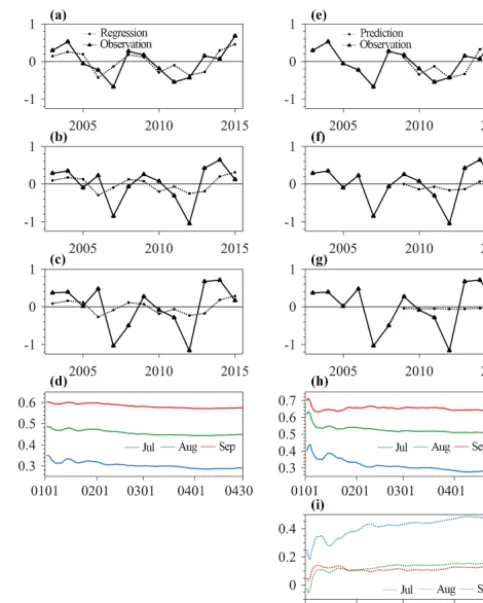
Figure 6a shows the regressed July Arctic sea ice extent anomalies. It appears that the observed interannual variabil-ity of July ASIE anomalies can be reasonably reproduced by the area of sea ice leads that is integrated from January to April. The regression error (root mean square error, RMSE) decreases gradually as the integration time period increases (blue line in Fig. 6d). The smallest error (0.28 million km2) occurs on 10 April, which is smaller than the standard devi-ation of the observed July sea ice extent during 2003–2015 (0.54 million km2). Figure 6b and c show the regressed Au-gust and September sea ice extent anomalies. The regressed August sea ice extent anomalies are off by a large margin for many years during 2003–2015 as compared to the ob-servations. This is also true for the regressed September sea ice extent anomalies. By the end of April, the error is 0.44 and 0.57 million km2for August (green line in Fig. 6d), and September (red line in Fig. 6d) respectively, which are com-parable to the standard deviation of the observed ones (0.60 and 0.73 million km2for August and September).
Figure 5. Evolution of correlation coefficients between the total area of sea ice leads integrated from 1 January to 30 April and the total Arctic sea ice extent in July (blue line), August (green line) and September (red line) during 2003–2015. The horizontal black dot line is the 99 % confidence level.
the slope and intercept of the linear regression model, and then Arctic sea ice extent anomalies during 2009–2015 are predicted using the corresponding integrated area of sea ice leads from January to April as inputs for the linear regression model. For July sea ice extent prediction (Fig. 6e), the evo-lution of the predicted ASIE anomalies is similar to the re-sult of the aforementioned regression (the observed variabil-ity of July ASIE anomalies during 2009–2015 is well cap-tured). As shown in Fig. 6h (blue line), the prediction error decreases gradually as the integration time period increases, and the error reaches 0.28 million km2 by the end of April which is smaller than the standard deviation of the observed July sea ice extent anomalies. For August and September sea ice extent prediction, the predicted sea ice extent anomalies cannot capture the observed ASIE anomalies, and the error is 0.51 and 0.63 million km2by the end of April for August and September, respectively. We also utilize the data from all pre-vious years to determine the slope and intercept of the linear regression model, and then calculate the Arctic sea ice extent anomalies during 2009-2015; i.e., the predicted July sea ice extent anomalies in 2009 (2015) are based on the training us-ing the data from 2003–2008 (2003–2014). The result of the predicted July sea ice extent anomalies is very similar to that using the data from the first 6 years (not shown).
Besides RMSE, the forecast skill (S) can be measured as follows:
S=1−σf σr ,
whereσf is the RMSE of the prediction error andσr is the RMSE of the observed July, August and September sea ice extent anomalies (with trend), respectively (0.54, 0.60 and 0.73 million km2 during 2003–2015). S that is equal to 1 means a perfect prediction, equal to and less than 0 implies no prediction skill. As shown in Fig. 6i, the prediction skill gradually increases with lengthening integration period. For July sea ice extent prediction, the predictive skill becomes
Figure 6.The total regressed Arctic sea ice extent anomalies (mil-lion km2) in(a)July,(b)August and(c)September on the area of sea ice leads integrated from 1 January to 30 April and(d)the evolu-tion of their regression errors. The total predicted Arctic sea ice ex-tent anomalies (million km2) in(e)July,(f)August and(g) Septem-ber based on the area of sea ice leads integrated from 1 January to 30 April,(h)the evolution of their prediction errors and(i)their forecast skills. The blue, green and red lines are July, August and September, respectively.
the highest in late April (0.49). By contrast, there is no pre-dictive skill for August and September sea ice extent. We also repeat this analysis by using the data from all previous years to determine the slope and intercept of the linear regression model. The result of the prediction skill is similar to Fig. 6 (not shown).
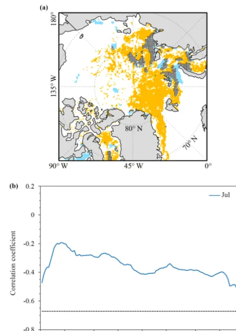
Figure 7.Evolution of correlation coefficients between the ATL-CWS region area of sea ice leads integrated from 1 January to 30 April and the ATLCWS region Arctic sea ice extent in July (blue line), August (green line) and September (red line) during 2003– 2015. The horizontal black dot line is the 99 % confidence level.
ice extent in the ATLCWS region, the correlation increases as the integration time period increases (blue line in Fig. 7). The strongest relationship occurs at day 68 (r= −0.78,>99 % significance) and then tends to level off until the end of April. For August sea ice extent (green line in Fig. 7), the evolution of the correlation coefficient is similar to that of July sea ice extent, and the correlation can reach−0.57 (>95 % signif-icance); it levels off until the end of April, which is much higher than that of pan-Arctic sea ice extent (r= −0.41). For September sea ice extent, though the relationship is better than the pan-Arctic result, the correlation is not statistically significant at the 95 % confidence level.
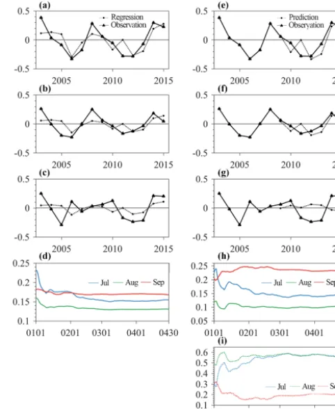
Following similar procedures in Fig. 6, we calculate the re-gression and prediction analyses, except that the area of sea ice leads in the ATLCWS region is integrated from 1 Jan-uary to 30 April 30. The results show that the observed interannual variability of July and August sea ice extent anomalies in the ATLCWS region can be reasonably repro-duced (Fig. 8a and b). The RMSE decreases gradually as the integration time period increases (blue and green lines in Fig. 8d). The smallest error occurs at day 68 for July (0.15 million km2) and day 68 (0.13 million km2) for August, which is smaller than the standard deviation of the observed sea ice extent during 2003–2015 (0.33 million km2 for July and 0.23 million km2 for August). The observed September sea ice extent anomalies in the ATLCWS region cannot be reproduced using the integrated sea ice leads in the same region. In terms of the prediction, as shown in Fig. 8h, the prediction error decreases gradually as the integration time period increases, and the error is 0.14 million km2 for July and 0.10 million km2 for August by the end of April. For September sea ice extent prediction, the predicted sea ice ex-tent anomalies cannot capture the observed anomalies.
Figure 8. The regressed ATLCWS region Arctic sea ice extent anomalies (million km2) in(a)July,(b) August and(c) Septem-ber on the ATLCWS region area of sea ice leads integrated from 1 January to 30 April and(d)the evolution of their regression er-rors. The predicted ATLCWS region Arctic sea ice extent anomalies (million km2) in(e)July,(f)August and(g)September based on the ATLCWS region area of sea ice leads integrated from 1 January to 30 April,(h)the evolution of their prediction errors and(i)their forecast skills. The blue, green and red lines are July, August and September, respectively.
4 Conclusion
Figure 9. (a)Spatial distribution of significant correlations between the area of clouds (blue) and sea ice leads (orange) integrated from 1 January to 30 April with July sea ice extent. Grey hatching denotes the overlapped significant correlations.(b)Evolution of correlation coefficients between the total area of cloud integrated from 1 Jan-uary to 30 April and the total Arctic sea ice extent in July (blue line) during 2003–2015. The horizontal line is the 99 % (black dot) confidence level.
To further ensure that the significant relationship between the area of sea ice leads and July sea ice extent is related to the area of sea ice leads actually present, rather than (1) cloud cover and (2) open water/polynyas in the marginal ice zone which can be wrongly classified as sea ice leads, first, we ex-amine the relationship between the area of clouds in the Arc-tic Ocean from late winter to mid-spring and ArcArc-tic sea ice extent during the melting season. Following the same pro-cedure applied to the calculation of sea ice leads as shown above, the area of clouds is defined as the sum of the product of the cloud fraction and the area of the grid box (625 km2) using the MOD08 daily cloud fraction data projected on the NSIDC polar-stereographic grid (25 km). We then calculate correlation coefficients between the de-trended time series of the integrated the area of (1) clouds and (2) open water at each grid point and the de-trended time series of the to-tal sea ice extent in July, respectively. Figure 9a shows
sig-Figure 10. (a) Spatial distribution of significant correlations be-tween the area of open water (blue) and sea ice leads (orange) in-tegrated from 1 January to 30 April with July sea ice extent. Grey hatching denotes the overlapped significant correlations.(b) Evolu-tion of correlaEvolu-tion coefficients between the total area of open water integrated from 1 January to 30 April and the total Arctic sea ice extent in July (blue line) during 2003–2015. The horizontal line is the 99 % (black dot) confidence level.
with the open water area, and the overlapped significant cor-relation only occurs in a small area (Fig. 10a). There is no significant correlation between the open water area and July sea ice extent (Fig. 10b). This suggests that the significant re-lationship between the area of sea ice leads and July sea ice extent is related to the area of actually present sea ice leads, rather than cloud cover or marginal ice zone open water.
Despite the potential of sea ice leads in the prediction of basin-wide and regional sea ice extent, sea ice leads consti-tute a largely unrepresented process in numerical prediction systems and climate models due to their highly nonlinear, small-scale, and intermittent features. As a result, the po-tential effects of sea ice leads on Arctic prediction are not well understood. Given that sea ice leads strongly influence the energy budget at the atmosphere–sea ice–ocean interface and the statistical results from this study, it would stand to reason that understanding the role of sea ice leads in Arctic prediction can identify performance limitations of numerical prediction systems and climate models and yield routes for significant improvements.
Data availability. All analyses in the study will be freely
avail-able to the public. Data requests can be sent to the first author (yyzhang@mail.bnu.edu.cn).
Author contributions. YZ processed and analyzed the data; YZ and
JL wrote the manuscript; XC and JL designed the experiments, in-vestigated the results and revised the manuscript; FH discussed the results. All authors provided substantial input to the interpretation of the results.
Competing interests. The authors declare that they have no conflict
of interest.
Acknowledgements. This research is supported by the
Na-tional Key R&D Program of China (2018YFA0605901 and 2016YFC1402704), the NOAA Climate Program Office (NA14OAR4310216), the NSFC (41676185), the China Schol-arship Council and the Fundamental Research Funds for the Central Universities. We also thank the NSIDC and PANGAEA for providing the data used in this study.
Edited by: Christian Haas
Reviewed by: two anonymous referees
References
Andreas, E., Paulson, C., William, R., Lindsay, R., and Businger, J.: The turbulent heat flux from Arctic leads, Bound.-Lay. Mete-orol., 17, 57–91, 1979.
Blanchard-Wrigglesworth, E., Cullather, R., Wang, W., Zhang, J., and Bitz, C.: Model forecast skill and sensitivity to initial
con-ditions in the seasonal Sea Ice Outlook, Geophys. Res. Lett., 42, 8042–8048, 2015.
Bröhan, D. and Kaleschke, L.: A nine-year climatology of Arctic sea ice lead orientation and frequency from AMSR-E, Remote Sens., 6, 1451–1475, 2014.
Budikova, D.: Role of Arctic sea ice in global atmospheric circula-tion: A review, Global Planet. Change, 68, 149–163, 2009. Cavalieri, D. J. and Parkinson, C. L.: Arctic sea ice
vari-ability and trends, 1979–2010, The Cryosphere, 6, 881–889, https://doi.org/10.5194/tc-6-881-2012, 2012.
Cavalieri, D. J., Parkinson, C. L., Gloersen, P., and Zwally, H. J.: Sea Ice Concentrations from Nimbus-7 SMMR and DMSP SSMI/I-SSMIS Passive Microwave Data, Version1, NASA Na-tional Snow and Ice Data Center Distributed Active Archive Cen-ter, Boulder, Colorado USA, 1996 (updated yearly).
Comiso, J. C., Parkinson, C. L., Gersten, R., and Stock, L.: Acceler-ated decline in the Arctic sea ice cover, Geophys. Res. Lett., 35, L01703, https://doi.org/10.1029/2007GL031972, 2008. Day, J., Hawkins, E., and Tietsche, S.: Will Arctic sea ice thickness
initialization improve seasonal forecast skill?, Geophys. Res. Lett., 41, 7566–7575, 2014.
Ding, Q., Schweiger, A., L’Heureux, M., Battisti, D. S., Po-Chedley, S., Johnson, N. C., Blanchard-Wrigglesworth, E., Harnos, K., Zhang, Q., and Eastman, R.: Influence of high-latitude atmo-spheric circulation changes on summertime Arctic sea ice, Nat. Clim. Change, 7, 289–295, 2017.
Dirkson, A., Merryfield, W. J., and Monahan, A.: Impacts of sea ice thickness initialization on seasonal Arctic sea ice predictions, J. Climate, 30, 1001–1017, 2017.
Drobot, S. D.: Using remote sensing data to develop seasonal out-looks for Arctic regional sea-ice minimum extent, Remote Sens. Environ., 111, 136–147, 2007.
Drobot, S. D., Maslanik, J. A., and Fowler, C.: A long-range fore-cast of Arctic summer sea-ice minimum extent, Geophys. Res. Lett., 33, L10501, https://doi.org/10.1029/2006GL026216, 2006. Eicken, H.: Ocean science: Arctic sea ice needs better forecasts,
Nature, 497, 431–433, 2013.
Forbes, B. C., Kumpula, T., Meschtyb, N., Laptander, R., Macias-Fauria, M., Zetterberg, P., Verdonen, M., Skarin, A., Kim, K.-Y., and Boisvert, L. N.: Sea ice, rain-on-snow and tundra rein-deer nomadism in Arctic Russia, Biol. Lett., 12, 20160466, https://doi.org/10.1098/rsbl.2016.0466, 2016.
Guemas, V., Blanchard-Wrigglesworth, E., Chevallier, M., Day, J. J., Déqué, M., Doblas-Reyes, F. J., Fuˇckar, N. S., Germe, A., Hawkins, E., and Keeley, S.: A review on Arctic sea-ice pre-dictability and prediction on seasonal to decadal time-scales, Q. J. Roy. Meteor. Soc., 142, 546–561, 2016.
Hamilton, L. C. and Stroeve, J.: 400 predictions: the SEARCH Sea Ice Outlook 2008–2015, Polar Geography, 39, 274–287, 2016. Holland, M. M. and Stroeve, J.: Changing seasonal sea ice predictor
relationships in a changing Arctic climate, Geophys. Res. Lett., 38, L18501, https://doi.org/10.1029/2011GL049303, 2011. Hubanks, P., Platnick, S., King, M., and Ridgway, B.: MODIS
Ivanova, N., Rampal, P., and Bouillon, S.: Error assessment of satellite-derived lead fraction in the Arctic, The Cryosphere, 10, 585–595, https://doi.org/10.5194/tc-10-585-2016, 2016. Kwok, R.: The RADARSAT Geophysical Processor System, in:
Analysis of SAR Data of the Polar Oceans: Recent Advances, edited by: Tsatsoulis, C. and Kwok, R., Springer-Verlag, New York, 235–257, 1998.
Kwok, R. and Cunningham, G.: Seasonal ice area and volume production of the Arctic Ocean: November 1996 through April 1997, J. Geophys. Res., 107, 8038, https://doi.org/10.1029/2000JC000469, 2002.
Lamers, M., Pristupa, A., Amelung, B., and Knol, M.: The changing role of environmental information in Arctic marine governance, Curr. Opin. Env. Sust., 18, 49–55, 2016.
Levermann, A., Mignot, J., Nawrath, S., and Rahmstorf, S.: The role of northern sea ice cover for the weakening of the thermo-haline circulation under global warming, J. Climate, 20, 4160– 4171, 2007.
Lindsay, R. and Rothrock, D.: Arctic sea ice leads from advanced very high resolution radiometer images, J. Geophys. Res.: 100, 4533–4544, 1995.
Lindsay, R., Zhang, J., Schweiger, A., and Steele, M.: Seasonal pre-dictions of ice extent in the Arctic Ocean, J. Geophys. Res., 113, C02023, https://doi.org/10.1029/2007JC004259, 2008.
Liu, J., Curry, J. A., Wang, H., Song, M., and Horton, R. M.: Impact of declining Arctic sea ice on winter snowfall, P. Natl. Acad. Sci. USA, 109, 4074–4079, 2012.
Liu, J., Song, M., Horton, R. M., and Hu, Y.: Reducing spread in climate model projections of a September ice-free Arctic, P. Natl. Acad. Sci. USA, 110, 12571–12576, 2013.
Liu, J., Song, M., Horton, R. M., and Hu, Y.: Revisiting the poten-tial of melt pond fraction as a predictor for the seasonal Arc-tic sea ice extent minimum, Environ. Res. Lett., 10, 054017, https://doi.org/10.1088/1748-9326/10/5/054017, 2015.
Lüpkes, C., Vihma, T., Birnbaum, G., and Wacker, U.: Influence of leads in sea ice on the temperature of the atmospheric bound-ary layer during polar night, Geophys. Res. Lett., 35, L03805, https://doi.org/10.1029/2007GL032461, 2008.
Marcq, S. and Weiss, J.: Influence of sea ice lead-width distribu-tion on turbulent heat transfer between the ocean and the atmo-sphere, The Cryoatmo-sphere, 6, 143–156, https://doi.org/10.5194/tc-6-143-2012, 2012.
Maykut, G. A.: Large-scale heat exchange and ice production in the central Arctic, J. Geophys. Res., 87, 7971–7984, 1982.
Miles, M. W. and Barry, R. G.: A 5-year satellite climatology of winter sea ice leads in the western Arctic, J. Geophys. Res., 103, 21723–21734, 1998.
Parkinson, C. L. and Comiso, J. C.: On the 2012 record low Arctic sea ice cover: Combined impact of preconditioning and an Au-gust storm, Geophys. Res. Lett., 40, 1356–1361, 2013.
Perovich, D., Grenfell, T., Light, B., and Hobbs, P.: Seasonal evolu-tion of the albedo of multiyear Arctic sea ice, J. Geophys. Res., 107, 8044, https://doi.org/10.1029/2000JC000438, 2002.
Richter-Menge, J., Overland, J., and Mathis, J.: Arctic Re-port Card, available at: https://arctic.noaa.gov/ReRe-port-Card/ Report-Card-2017 (last access: 21 November 2018), 2016. Röhrs, J. and Kaleschke, L.: An algorithm to detect sea ice leads by
using AMSR-E passive microwave imagery, The Cryosphere, 6, 343–352, https://doi.org/10.5194/tc-6-343-2012, 2012.
Schröder, D., Feltham, D. L., Flocco, D., and Tsamados, M.: September Arctic sea-ice minimum predicted by spring melt-pond fraction, Nat. Clim. Change, 4, 353–357, 2014.
Spreen, G., Kwok, R., Menemenlis, D., and Nguyen, A. T.: Sea-ice deformation in a coupled ocean-sea-ice model and in satellite remote sensing data, The Cryosphere, 11, 1553–1573, https://doi.org/10.5194/tc-11-1553-2017, 2017.
Stroeve, J., Holland, M. M., Meier, W., Scambos, T., and Serreze, M.: Arctic sea ice decline: Faster than forecast, Geophys. Res. Lett., 34, L09501, https://doi.org/10.1029/2007GL029703, 2007. Stroeve, J., Hamilton, L. C., Bitz, C. M., and Blanchard-Wrigglesworth, E.: Predicting September sea ice: Ensemble skill of the SEARCH sea ice outlook 2008–2013, Geophys. Res. Lett. 41, 2411–2418, 2014.
Stroeve, J. C., Serreze, M. C., Holland, M. M., Kay, J. E., Malanik, J., and Barrett, A. P.: The Arctic’s rapidly shrinking sea ice cover: a research synthesis, Climatic Change, 110, 1005–1027, 2012. Tschudi, M., Curry, J., and Maslanik, J.: Characterization of
spring-time leads in the Beaufort/Chukchi Seas from airborne and satel-lite observations during FIRE/SHEBA, J. Geophys. Res., 107, 8034, https://doi.org/10.1029/2000JC000541, 2002.
Vihma, T.: Effects of Arctic sea ice decline on weather and climate: a review, Surv. Geophys., 35, 1175–1214, 2014.
Wadhams, P., McLaren, A. S., and Weintraub, R.: Ice thickness dis-tribution in Davis Strait in February from submarine sonar pro-files, J. Geophys. Res., 90, 1069–1077, 1985.
Wang, Q., Danilov, S., Jung, T., Kaleschke, L., and Wernecke, A.: Sea ice leads in the Arctic Ocean: Model assessment, interannual variability and trends, Geophys. Res. Lett., 43, 7019–7027, 2016. Wernecke, A. and Kaleschke, L.: Lead detection in Arctic sea ice from CryoSat-2: quality assessment, lead area frac-tion and width distribufrac-tion, The Cryosphere, 9, 1955–1968, https://doi.org/10.5194/tc-9-1955-2015, 2015.
Willmes, S. and Heinemann, G.: Pan-Arctic lead detection from MODIS thermal infrared imagery, Ann. Glaciol., 56, 29–37, 2015a.
Willmes, S. and Heinemann, G.: Daily pan-Arctic sea-ice lead maps for 2003–2015, with links to maps in NetCDF format, PAN-GAEA, https://doi.org/10.1594/PANGAEA.854411, 2015b. Willmes, S. and Heinemann, G.: Sea-ice wintertime lead