the Creative Commons Attribution 4.0 License.
Greenland iceberg melt variability from high-resolution
satellite observations
Ellyn M. Enderlin1,2, Caroline J. Carrigan2, William H. Kochtitzky1,2, Alexandra Cuadros3, Twila Moon4, and Gordon S. Hamiltona,b,†
1Climate Change Institute, University of Maine, Orono, ME 04469, USA
2School of Earth and Climate Sciences, University of Maine, Orono, ME 04469, USA 3School of Marine Sciences, University of Maine, Orono, ME 04469, USA
4National Snow and Ice Data Center, University of Colorado, Boulder, CO 80303, USA aformerly at: Climate Change Institute, University of Maine, Orono, ME 04469, USA
bformerly at: School of Earth and Climate Sciences, University of Maine, Orono, ME 04469, USA †deceased
Correspondence:Ellyn M. Enderlin (ellyn.enderlin@gmail.com) Received: 28 August 2017 – Discussion started: 21 September 2017
Revised: 9 January 2018 – Accepted: 11 January 2018 – Published: 20 February 2018
Abstract. Iceberg discharge from the Greenland Ice Sheet accounts for up to half of the freshwater flux to surround-ing fjords and ocean basins, yet the spatial distribution of iceberg meltwater fluxes is poorly understood. One of the primary limitations for mapping iceberg meltwater fluxes, and changes over time, is the dearth of iceberg submarine melt rate estimates. Here we use a remote sensing approach to estimate submarine melt rates during 2011–2016 for 637 icebergs discharged from seven marine-terminating glaciers fringing the Greenland Ice Sheet. We find that spatial vari-ations in iceberg melt rates generally follow expected pat-terns based on hydrographic observations, including a de-crease in melt rate with latitude and an inde-crease in melt rate with iceberg draft. However, we find no longitudinal vari-ations in melt rates within individual fjords. We do not re-solve coherent seasonal to interannual patterns in melt rates across all study sites, though we attribute a 4-fold melt rate increase from March to April 2011 near Jakobshavn Isbræ to fjord circulation changes induced by the seasonal onset of iceberg calving. Overall, our results suggest that remotely sensed iceberg melt rates can be used to characterize spatial and temporal variations in oceanic forcing near often inac-cessible marine-terminating glaciers.
1 Introduction
The Greenland Ice Sheet discharges ∼550 Gt of icebergs per year (Enderlin et al., 2014). This accounts for approximately a third to a half of the total freshwater flux from Greenland to the surrounding fjords and ocean basins (Bamber et al., 2012; Enderlin et al., 2014; van den Broeke et al., 2016). Unlike surface meltwater runoff fluxes from the ice sheet and tundra, which primarily enter the ocean system from point sources (subglacial discharge channels and terrestrial rivers, respec-tively), icebergs act as distributed freshwater sources. The spatial distribution of iceberg freshwater fluxes is dependent on a number of factors, including the volume and size distri-bution of ice calved from each glacier, which varies substan-tially over a range of spatial scales (Enderlin et al., 2014), and the solid-to-liquid conversion rate of an iceberg’s freshwa-ter reserves. Although surface sublimation and melting, wave erosion, and submarine melting all contribute to iceberg ab-lation, the solid-to-liquid conversion rate should primarily be dictated by submarine melting because of the strong depen-dence of total ablation on the surface area over which each process acts (e.g., Enderlin et al., 2016; Moon et al., 2017).
a
Easting (km)
-600 -400 -200 0 200 400 600 800
Northing (km)
-3250 -3000 -2750 -2500 -2250 -2000 -1750 -1500 -1250 -1000
Kong Oscar Alison Upernavik Jakobshavn Zachariae Helheim Koge Bugt
5 km
b
c
d
e
f
g
h
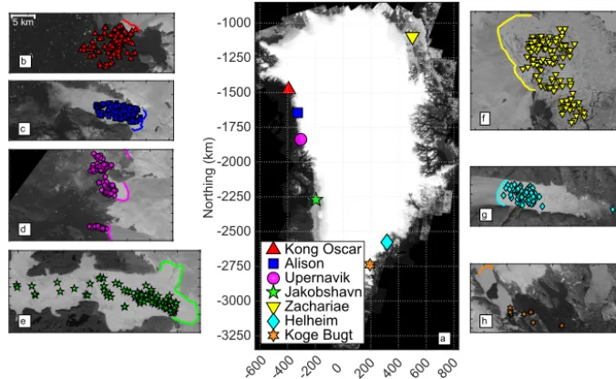
Figure 1.Location of Greenland icebergs included in this study.(a)The locations of the glaciers from which the icebergs calved overlain on the GIMP image mosaic. The different iceberg sources are distinguished by symbol color and shape (see legend).(b–h)Locations of all study icebergs overlain on summer 2016 Landsat 8 panchromatic images of(b)Kong Oscar Glacier,(c)Alison Glacier,(d)Upernavik Glacier,(e)Jakobshavn Isbræ,(f)Zachariæ Isstrøm,(g)Helheim Glacier, and(h)Koge Bugt Glacier. The same scale, shown in panel(b), is used in panels(b–h). Termini of the icebergs’ glacier sources are delineated with colored lines in panels(b–h).
and Dowdeswell, 2010; Enderlin et al., 2016). The location where iceberg meltwater enters the ocean system is prov-ing important for local to global ocean circulation (Luo et al., 2016; Stern et al., 2016), yet the spatial distribution of iceberg meltwater fluxes has been largely overlooked be-cause it cannot be estimated from existing hydrographic ob-servations (Jackson and Straneo, 2016). Where iceberg res-idence times can be estimated from, for example, iceberg tracking (Sulak et al., 2017), these data can be paired with re-motely sensed iceberg size and area distributions (Enderlin et al., 2016; Sulak et al., 2017) and empirical iceberg melt rates to estimate iceberg freshwater fluxes. However, there are only a handful of locations around Greenland where there are sufficient water temperature and velocity records to constrain empirical iceberg melt rate estimates in iceberg-congested fjords (e.g., Bendtsen et al., 2015; Gladish et al., 2015; Jack-son and Straneo, 2016). To address the dearth of iceberg melt rate estimates in Greenland’s fjords, here we use a satel-lite remote sensing method to construct time series of sub-marine melt rates and meltwater fluxes for icebergs calved from seven large outlet glaciers spanning the periphery of the Greenland Ice Sheet (Fig. 1). Although the iceberg melt esti-mates constructed using this remote sensing method are lim-ited to irregular observation periods during 2011–2016, the data provide the most comprehensive observationally con-strained estimates of Greenland iceberg melting to date.
2 Methods
As a freely floating iceberg ablates, the elevation of its sur-face lowers in proportion to the iceberg’s volume loss so that the iceberg remains in hydrostatic balance with the water in which it is submerged. This principle enables the estimation of iceberg meltwater fluxes (i.e., volume lost due to subma-rine melting per unit time) from repeat remotely sensed sur-face elevation observations. Here we follow the approach of Enderlin and Hamilton (2014) to estimate changes in surface elevation using very high-resolution stereo satellite images acquired by the WorldView constellation of satellites. We note that this method could also be applied to elevation time series from terrestrial laser scanners, stereo imagery acquired by unmanned aerial vehicles or other satellite platforms, or GPS-derived elevations, but we focus on WorldView data be-cause, unlike data acquired from the other platforms, World-View data can be used to construct multi-year records of iceberg elevation change around the entire ice sheet periph-ery. Using this approach, we produce iceberg melt estimates from multiple observation periods during 2011–2016 (Fig. 1, Table 1) for seven large marine-terminating glaciers across southeast, northeast, and western Greenland that have suf-ficient WorldView image archives to estimate iceberg melt rates for more than one observation period.
high-Table 1.Overview of iceberg observations and derived melt rate parameterizations for each study site. Column 1: glacier names; columns 2– 3: observation periods; column 4: number of observations; column 5: number of observations per 50 m draft bin for each observation period (listed from 0–50 to 350–400 m depths); and column 6: meltwater flux parameterizations. In column 5, the correlation coefficients and root mean square error estimates for the linear area-based meltwater flux parameterizations are also provided.
Glacier Year Period Observations Observations per 1V / 1t=f (Asub)
50 m draft bin
2012 14–26 Apr 22 0, 5, 6, 5, 4, 0, 1, 0 26 Apr–11 Jun 20 0, 0, 7, 6, 4, 1, 1, 0
2014 4 May–13 Jun 18 1, 7, 7, 0, 3, 0, 0, 0 13 Jun–4 Aug 3 0, 0, 0, 1, 1, 0, 0, 0
Kong Oscar
2015
6–19 Apr 13 0, 6, 4, 1, 1, 0, 0, 0 0.209A-38413 (R=0.85, RMSE=40 447) 12 May–11 Jun 13 0, 1, 8, 2, 1, 0, 0, 0
11 Jun–12 Aug 7 0, 0, 2, 1, 1, 1, 1, 0
2016 18 Mar–19 May 16 0, 4, 8, 3, 0, 0, 0, 0 19 May–20 Jul 4 0, 1, 1, 1, 1, 0, 0, 0
2011 25 Mar–11 Apr 19 5, 8, 5, 0, 0, 0, 0, 0 11 Apr–10 Jun 24 7, 13, 2, 1, 0, 0, 0, 0
2013
10 Apr–12 May 16 1, 6, 4, 2, 1, 1, 0, 0
Alison 12 May–22 Jun 18 0, 5, 6, 3, 1, 2, 0, 0 0.140A-13878 (R=0.69, RMSE=24 120) 22 Jun–7 Jul 25 2, 10, 7, 2, 1, 2, 0, 0
7–22 Jul 22 0, 6, 7, 2, 3, 3, 0, 0
2016 8 May–14 Jul 16 0, 4, 8, 4, 0, 0, 0, 0
2011 26 Mar–12 Apr 21 3, 10, 5, 1, 1, 0, 0, 0
2013 12–30 Apr 17 4, 6, 4, 0, 0, 1, 1, 0
Upernavik 30 Apr–3 Jun 16 5, 8, 0, 0, 0, 1, 1, 0 0.248A-31052 (R=0.88, RMSE=61 611)
2014 28 Mar–17 Apr 20 0, 10, 4, 2, 2, 1, 0, 0
2016 16 –27 Apr 9 0, 2, 5, 1, 0, 1, 0, 0
2011 19 Mar–6 Apr 22 0, 2, 3, 9, 5, 1, 0, 1 6–11 Apr 14 0, 2, 2, 7, 0, 1, 1, 0
2012 13–16 Jul 13 0, 4, 7, 1, 0, 0, 0, 0 Jakobshavn
2014
30 Mar–19 Apr 19 0, 3, 6, 5, 1, 2, 1, 0 0.338A-34434 (R=0.74, RMSE=74 454) 18–30 Jun 6 0, 1, 1, 3, 0, 0, 0, 0
30 Jun–18 Jul 3 0, 0, 1, 1, 0, 0, 0, 0
2015 31 Jul–13 Aug 8 0, 3, 4, 0, 1, 0, 0, 0
2011 31 May–8 Jun 21 1, 4, 14, 1, 0, 0, 0, 0 8 Jun–10 Jul 24 2, 6, 14, 1, 0, 0, 0, 0
2013
1 Apr–5 Jun 23 0, 8, 9, 3, 2, 0, 0, 0
Zachariæ 5 Jun–25 Jul 27 0, 12, 2, 5, 6, 1, 0, 0 0.118A-23772 (R=0.75, RMSE=43 816) 25 Jul–10 Aug 15 1, 2, 2, 2, 5, 2, 0, 0
2015 1 Apr–1 May 17 0, 0, 0, 9, 3, 3, 1, 0 2 Jun–2 Jul 9 0, 0, 1, 3, 2, 1, 1, 1
2011 21–24 Aug 3 0, 1, 0, 1, 0, 0, 0, 0
2012 24–29 Jun 18 0, 5, 6, 4, 1, 1, 0, 0
Helheim
2014 2–31 Jul 20 1, 7, 7, 3, 0, 1, 0, 0 0.363A-37746 (R=0.84, RMSE=53 704) 16–30 Oct 14 0, 1, 4, 6, 1, 1, 0, 0
2015 10–16 Aug 16 0, 3, 8, 4, 1, 0, 0, 0
resolution (2 m horizontal resolution, ∼3 m vertical uncer-tainty; Enderlin and Hamilton, 2014) digital elevation mod-els (DEMs) of iceberg-congested waters. A comparison of the DEMs produced using the SETSM and ASP algorithms indicates that the accuracy of iceberg elevations derived from the algorithms is comparable, allowing us to switch from the use of SETSM DEMs for 2011–2014 images to ASP DEMs for 2015–2016 images without biasing our results. DEMs were constructed over the entire stereo image domain so that bedrock and water surface elevations could be used to co-register DEMs (Enderlin and Hamilton, 2014).
To estimate the change in iceberg volume between image acquisition dates, we applied the same DEM-differencing approach as Enderlin and Hamilton (2014) and Enderlin et al. (2016): changes in iceberg surface elevation were man-ually extracted from repeat co-registered DEMs, then con-verted to estimates of iceberg volume change under the as-sumption of hydrostatic equilibrium. The contribution of ice-berg surface melting to the observed volume change was estimated from the daily runoff time series for the nearest glaciated pixel in the Regional Atmospheric Climate Model (RACMO) for Greenland (van Meijgaard et al., 2008; van Angelen et al., 2014; van den Broeke, 2017), then subtracted from the ice volume change estimates to yield ice volume loss due to submarine melting. Although there are slight differences in runoff estimates generated by RACMO v2.3 (used for 2011–2014) and v2.4 (used for 2015–2016), the version of RACMO used in our analysis had no apprecia-ble influence on ice volume loss partitioning because volume loss due to surface melting constituted <5 % of total vol-ume change. We converted our estimates of ice volvol-ume lost via submarine melting to estimates of liquid freshwater flux (cubic meters of meltwater produced per day) and average submarine melt rates (meters per day) over the submerged iceberg areas. To estimate the average draft (i.e., keel depth) and submerged area of each iceberg, we assumed that the submerged iceberg shapes can be approximated by cylinders with dimensions defined by the iceberg surface elevation and surface area estimates (Enderlin and Hamilton, 2014). Under this assumption, the draft (d) is estimated as
d= ρi
ρsw−ρi
z, (1)
and the area-averaged melt rate (m˙) is estimated as
˙
m= 1V
1t
2π rd+π r2, (2)
wherezis the median ice surface elevation,ρiandρsware the ice and sea water densities, respectively,1V is the change in volume between image acquisition dates,1t is the time be-tween image acquisition dates, andris the average radius of the iceberg surface in each image pair. Submerged iceberg shapes are likely to be more complex than the cylindrical shapes used herein but are impossible to discern from sur-face observations alone. However, good agreement among
iceberg melt rates derived via DEM differencing and em-pirical melt rate estimates in Helheim’s fjord (Enderlin and Hamilton, 2014; FitzMaurice et al., 2016; Moon et al., 2017) suggests that submerged iceberg shapes can be reasonably approximated by cylinders.
Uncertainties in the submarine meltwater flux, submerged area, draft, and melt rate estimates are described in detail in Enderlin and Hamilton (2014) and is, therefore, only sum-marized briefly here. All errors are propagated through our calculations, then summed in quadrature. Potential errors arise from (1) surface elevation errors, (2) uncertainty in the operator-defined iceberg tracking, (3) uncertainties/changes in the ice and ocean water densities used to convert elevation change to volume change, (4) surface melt over- or underes-timation, and (5) changes in the iceberg surface area between image acquisitions. Systematic and random errors in iceberg elevations are minimized through vertical co-registration of iceberg DEMs using neighboring open water elevations and through spatial averaging, respectively. Uncertainties intro-duced by manual translation and rotation of iceberg masks in repeat DEMs are quantified through repeated delineation of each iceberg. Ice and water densities are assumed to vary by up to 10 and 2 kg m−3, respectively, between observations. A conservative surface meltwater uncertainty of 30 % is ap-plied to account for RACMO uncertainties and potential de-viations in the melt rate of icebergs from the nearest glacier-ized RACMO grid cell. The surface area uncertainty is de-fined as the temporal range about the mean. The typical (i.e., median) uncertainties in the submarine meltwater flux, draft, submerged area, and melt rate are 25.6, 2.7, 3.2, and 27.6 %, respectively.
Figure 2.Liquid freshwater fluxes (millions of cubic meters per day) plotted against the estimated submerged area (square kilometers) for all icebergs sampled near the terminus of(a)Kong Oscar Glacier,(b)Alison Glacier,(c)Upernavik Glacier,(d)Jakobshavn Isbræ,(e)Zachariæ Isstrøm,(f)Helheim Glacier, and(g)Koge Bugt Glacier. Vertical error bars indicate the meltwater flux uncertainties due to random DEM errors, ice density uncertainties, surface meltwater flux uncertainties, and manual iceberg delineation errors. Horizontal error bars indicate the range of submerged iceberg areas predicted for cylindrical submerged geometries using surface elevation and map-view surface area estimates extracted from repeat DEMs. Linear polynomials fit to the datasets compiled for each study site are plotted as thick colored lines and the surrounding shaded envelopes encompass their 95 % confidence intervals. Area-averaged submarine melt rates derived from the polynomials are listed in each panel.
submerged geometries, we are confident that any changes in iceberg submerged geometries over the timescales consid-ered here are reasonably captured by our submerged area un-certainty estimates.
3 Results and discussion
We extracted a total of 637 iceberg meltwater flux and melt rate estimates near the termini of seven large marine-terminating outlet glaciers fringing the Greenland Ice Sheet periphery and spanning March–October of 2011–2016 (Ta-ble 1; Enderlin, 2017). The number of estimates varies widely, with 3 to 27 melt estimates per observation pe-riod (mean=15). In general, the number of estimates is in-versely proportional to the distance between the icebergs and their parent glaciers and the time period between im-age acquisitions, restricting our analysis to icebergs located within ∼10 km of the glacier termini and to time spans of 3–67 days.
3.1 Regional patterns
the central west (∼0.14–0.24 m d−1). The lowest melt rates are found for icebergs calved from Zachariæ Isstrøm in the northeast (∼0.12 m d−1).
The observed large-scale spatial patterns in melt rate gen-erally follow expected variations based on regional differ-ences in subsurface ocean temperatures (e.g., Straneo et al., 2012) and surface meltwater runoff (e.g., van den Broeke et al., 2016), which drives summertime fjord circulation (Jackson and Straneo, 2016). There are, however, some no-table exceptions. The average melt rate estimate for Koge Bugt is nearly double the average melt rate for icebergs calved from Helheim Glacier despite similar water temper-atures near the fjord mouths (Sutherland et al., 2013). Al-though our Koge Bugt dataset includes only seven icebergs across two observation periods, we observe melt rates of
>0.6 m d−1during both observation periods, increasing our confidence that the difference in average melt rates reflects variations in typical melt conditions at the two study sites and is not due to observational uncertainties or anomalous melt conditions. We also find a discrepancy in the predicted latitu-dinal decrease in the iceberg melt rates in northwest Green-land, where we observe lower melt rates for icebergs calved from Alison Glacier than the more northerly Kong Oscar Glacier. We hypothesize that the strengthened latitudinal gra-dient in the southeast and reversed gragra-dient in the northwest are due to spatial variations in turbulent melting below the waterline associated with differences in near-surface water temperatures and/or relative velocity (i.e., difference in wa-ter and iceberg velocities) for icebergs located in kilomewa-ters- kilometers-long iceberg-congested fjords (Helheim and Alison) versus freely floating icebergs in close proximity to the open ocean (Koge Bugt and Kong Oscar). Additional in situ water tem-perature and velocity observations are required to test this hypothesis, but if proven true, it suggests that near-terminus hydrography is strongly influenced by fjord geometry. 3.2 Local patterns
Although detailed in situ hydrographic analyses of Green-land’s glacial fjords are limited in space and time, existing observations indicate that there are much steeper gradients in water temperature and velocity in the vertical plane (i.e., with depth) than in the horizontal plane (i.e., along fjord) (Sutherland et al., 2014; Bendtsen et al., 2015; Gladish et al., 2015; Jackson and Straneo, 2016). As such, we expect to find pronounced variations in melt rates for icebergs that do and do not penetrate into the relatively warm and salty wa-ter masses found below∼100–200 m depth around the ice sheet periphery (Straneo et al., 2012; Moon et al., 2017) but no discernible variations in melt rates with distance from the parent glacier.
To examine the depth dependency of iceberg melt rates, we first sorted the icebergs according to their median draft. After parsing the icebergs into 50 m increment draft bins, we calcu-lated the medians of all the area-averaged melt rate estimates
(hereafter the median melt rate) and draft estimates in each bin. Figure 3 shows the binned median melt rates and drafts for each study site. For all study sites, the median melt rates are generally smaller for icebergs in the upper∼200 m of the water column than those that penetrate to greater depths (Fig. 3a, b–h). The depth dependency of iceberg melt rates is particularly pronounced for icebergs calved from the Uper-navik glaciers (Fig. 3d) and Jakobshavn Isbræ (Fig. 3e) in the central west. For Upernavik, the median melt rate increases from the surface down to∼150 m depth, decreases slightly over the 150–200 m depth range, then increases again below 200 m depth. For Jakobshavn, the median melt rate increases from the surface down to∼150 m depth, decreases down to
∼250 m depth, then increases again down to 350 m depth. The apparent decrease in the melt rate below 350 m depth reflects one observation from March 2011, when melt rates were particularly low, as discussed more below. Although the dip in melt rates at∼200 m depth is not significant (i.e., does not exceed the uncertainty of neighboring bins), it co-incides with the approximate depth of the interface between the colder near-surface waters and warmer subsurface wa-ters observed in Jakobshavn’s fjord (Ilulissat Icefjord) (Glad-ish et al., 2015) and the Upernavik fjord system (Fenty et al., 2016), where water velocities should be relatively slow and turbulent melting should reach a local minimum (Moon et al., 2017). These observations suggest that our remote sensing method may be capable of resolving the depth of the near- and subsurface water interface where hydrographic ob-servations are difficult or impossible to acquire, such as near the termini of calving glaciers. However, we caution that the area-averaged melt rates obtained using this approach likely underestimate the trend of increasing melt rates with depth because of the integrative nature of our area-averaged melt rate estimates.
3.3 Temporal patterns
coher-Iceberg draft (m b.s.l.)
0 100 200 300 400
Normalized melt ra
-1 -0.5 0 0.5 1
(a)
0 0.2 0.4 0.6
0.8 (b) (f)
0 0.2 0.4 0.6
0.8 (c) (g)
0 0.2 0.4 0.6
0.8 (d)
Iceberg draft (m b.s.l.)
0 100 200 300 400
(h)
Iceberg draft (m b.s.l.)
0 100 200 300 400
Area-averaged melt rate (m d )
0 0.2 0.4 0.6
0.8 (e)
Kong Oscar Alison Upernavik Jakobshavn Zachariae Helheim Koge Bugt
-1
Figure 3.Plots of melt rate variability with draft.(a)Normalized melt rate plotted against median draft (meters below sea level). Normalized melt rates less than zero are below the observed average and values greater than zero indicate above-average melt rates.(b–h)Area-averaged melt rate (meters per day) plotted against median draft (meters below sea level) for icebergs near the terminus of(b)Kong Oscar Glacier, (c)Alison Glacier,(d)Upernavik Glacier,(e)Jakobshavn Isbræ,(f)Zachariæ Isstrøm,(g)Helheim Glacier, and(h)Koge Bugt Glacier. In all panels, icebergs are sorted into 50 m increment draft bins and the symbols mark the median values for each draft bin. In(b–h), vertical error bars bound the range of melt rates.
ent temporal signal across all study sites does not preclude the existence of temporal variations.
Our finding that, overall, there is no seasonal or inter-annual variation is in contrast to empirical melt estimates, which suggest there should be pronounced seasonal differ-ences in iceberg melt rates (Mugford and Dowdeswell, 2010) primarily due to the strong dependency of iceberg melt-ing on water velocities (Bigg et al., 1997; FitzMaurice et al., 2016, 2017). The lack of substantial coherent temporal variability in our iceberg melt rate estimates may be influ-enced by a number of factors. First, the number of repeat DEMs and timing of DEM acquisitions varies substantially from year to year and between study sites, making it difficult to infer seasonal and interannual patterns from our dataset. Second, our remotely sensed melt rates integrate variations in melt rate with depth and over the time interval between DEM acquisition dates. The depth integration likely has lit-tle influence on shallow-drafted icebergs that are bathed in relatively homogeneous water but may substantially reduce the melt rates for deep-drafted icebergs, as previously men-tioned. The time-integrative nature of our remotely sensed melt rates means that high-frequency variations in iceberg melting are smoothed out. Temporal smoothing is likely to be particularly important during the seasonal transition from winter conditions (i.e., expansive sea ice, little subglacial
meltwater discharge, synoptic-scale changes in fjord circula-tion) to summer conditions (i.e., open water with fjord circu-lation driven by subglacial discharge) (Jackson et al., 2014), which may lead to rapid changes in submarine melt rates. Finally, uncertainties in the melt rate estimates introduced by observational uncertainties, particularly uncertainty in the submerged iceberg shape, may also partially obscure tem-poral variations in iceberg melting over seasonal to inter-annual timescales. While our results here validate our use of time-averaged melt rates in the spatial analyses presented above, further research on temporal variations in iceberg melt is necessary to determine whether changes in iceberg melt-water fluxes over time have an appreciable impact on local-to-regional ocean circulation, motivating the need for more detailed time series of iceberg melt rates around Greenland.
0 0.2 0.4 0.6
0.8 (a) (e)
0 0.2 0.4 0.6
0.8 (b)
(f)
0 0.2 0.4 0.6
0.8 (c)
Iceberg draft (m b.s.l.)
0 100 200 300 400
(g)
Iceberg draft (m b.s.l.)
0 100 200 300 400
Area-averaged melt rate (m d )
0 0.2 0.4 0.6
0.8 (d)
March April May June July August September October
2011 2012 2013 2014 2015 2016
-1
Figure 4.Area-averaged iceberg melt rate (meters per day) plotted against median draft (meters below sea level) for icebergs sampled near the terminus of(a)Kong Oscar Glacier,(b)Alison Glacier,(c)Upernavik Glacier,(d)Jakobshavn Isbræ,(e)Zachariæ Isstrøm,(f)Helheim Glacier, and(g)Koge Bugt Glacier. For each observation period, icebergs were organized into 50 m deep draft bins and the median melt rate and draft were computed. The symbols mark the median values and the error bars mark the range of estimates for each draft bin. The face colors and edge colors of the symbols indicate the year and month of the observations, respectively (see legends).
Icefjord between late March and early April 2011 (Fig. 5). This rapid increase in iceberg melting coincided with the appearance of distinct lateral shear margins in the 6 April WorldView image of the fjord’s extensive ice mélange, which were not present in a 19 March WorldView image. Surface air temperatures observed at the closest on-ice automatic weather station (673 m a.s.l.; 67.097◦N, 49.933◦E) lapsed to sea level indicate that regional air temperatures were well be-low freezing (daily mean temperatures<−10◦C) for 20 of
24 days between the image acquisitions; thus, the appearance of the shear margins cannot be easily explained by surface melting. We suggest that shear margins instead appeared as a result of abrupt mélange motion away from the terminus during a large calving event. Seismic data recorded in Ilulis-sat, at the fjord mouth, confirm that the earliest large-scale calving event of 2011 occurred on 3 April, 3 days prior to the beginning of our second observation period.
Based on the large change in deep-drafted melt rates and coincident onset of seasonal calving, we hypothesize that ice-berg overturning during the calving event altered the strat-ification and circulation of the fjord water masses, which rapidly increased iceberg melt rates at depth. Although the size of the calving event and the degree of mixing within
the water column are unknown, laboratory experiments of iceberg overturning indicate that the amount of energy re-leased during a large calving event is far more than enough to entirely mix the water column within 1 km of Jakobshavn’s terminus (Burton et al., 2012). To assess whether mixing-induced changes in water temperature or velocity was the more likely driver of the observed change in melt rate, we turn to the thermodynamic equations of submarine melting. Turbulent melting due to horizontal water shear past an ice-berg is estimated as
˙
mturbulent=0.58v0.8
Tsw−Ti
L0.2 , (3)
and buoyancy-driven melting is
˙
mbuoyant=
7.62×10⁻³Tsw+
Figure 5.Area-averaged submarine melt rates plotted against me-dian draft for icebergs calved from Jakobshavn Isbræ, west Green-land, into Ilulissat Icefjord. As in Fig. 4, the symbols mark the me-dian values and the error bars mark the range of estimates for each draft bin. The face colors and edge colors of the symbols indicate the year and month of the observations, respectively, as described in the legend. The large increase in the area-averaged melt rate below 150 m depth from March to April in 2011 are highlighted by the shaded rectangles. The dashed lines within the rectangles mark the average melt rates for icebergs with drafts>150 m and the differ-ence in the average melt rate between observation periods is denoted by the double-sided arrow.
drive the 4-fold increase in deep-drafted melt rates. How-ever, for an ice temperature of−5◦C (Vieli and Nick, 2011) and a water temperature of 2◦C (Gladish et al., 2015), the relative velocity would need to increase from an average of approximately 0.06 to 0.31 m s−1to increase the turbulence-driven melt rate of large (∼500 m long) icebergs from∼0.12 to∼0.46 m d−1. The persistent ice mélange near the Jakob-shavn terminus prevents acquisition of the water temperature and velocity time series required to test this hypothesis. How-ever, water velocity data from Sermilik Fjord in southeast Greenland suggest that velocities of≥0.3 m s−1(Jackson et al., 2014) are possible in Greenland’s deep glacial fjords. Moreover, given the mostly below-freezing air temperatures observed over this period of rapid change (PROMICE, 2017), it is unlikely that the inferred changes in fjord circulation were triggered by the seasonal onset of glacier meltwater-enhanced subglacial discharge at depth in the fjord. There-fore, we interpret the 4-fold increase in melt rates as an in-dication that full-thickness calving events from large glacier termini may significantly alter the hydrographic properties of Greenland’s glacial fjords, with a measurable influence on iceberg melt.
Here we apply a remote sensing method to construct sub-marine melt rate and meltwater flux time series for icebergs calved from seven large marine-terminating outlet glaciers spanning the Greenland Ice Sheet edge. We find that for each study site, the meltwater flux from icebergs can be reason-ably approximated as a linear function of the submerged ice-berg area. Differences in the rate of iceice-berg melting between study sites generally follow expected geographic patterns based on variations in ocean temperature and surface melt-water runoff from the ice sheet, with the highest melt rates in the southeast, decreasing melt rates with increasing latitude along the west coast, and the lowest melt rates in the north-east. We hypothesize that deviations from the expected lati-tudinal patterns are due to variations in the prevalence of ice-bergs and/or near-terminus water circulation associated with different fjord geometries, emphasizing the potential impor-tance of Greenland fjord geometry on iceberg (and glacier) melt rates.
At finer spatial scales, our observations support the ex-pected depth dependency of iceberg melt rates in the highly stratified water fringing Greenland: at each study site, melt rates are low and fairly uniform down to∼200 m depth then gradually increase down to∼350 m below the sea surface. Although our melt rate time series across all study sites do not reveal coherent temporal variations in melting, obser-vations compiled for Jakobshavn Isbræ’s fjord suggest that abrupt changes in melt conditions do occur. Furthermore, these changes at depth can potentially be monitored using the remote sensing approach applied here. The data com-piled for Jakobshavn Isbræ also suggest that full-thickness calving events may be important for fjord circulation and ice-berg melt, though additional melt rate estimates with approx-imately weekly temporal resolution, possibly from terrestrial laser scanner or unmanned aerial vehicle observations, are required to test the effect of calving on subsurface melt con-ditions.
Data availability. The location, median surface elevation, surface elevation uncertainty, and vertical co-registration for each obser-vation date and estimates of the ice volume change rate, un-certainty in the ice volume change rate, average draft, range in draft, average surface area, range in surface area, average sub-merged area, and range in subsub-merged area between observa-tion dates for all icebergs in our analysis can be accessed at https://doi.org/10.18739/A20N7C. RACMO Greenland v2.3 runoff data for 2011–2014 and v2.4 runoff data for 2015–2016 were provided by Michiel van den Broeke, Utrecht University (https:// www.projects.science.uu.nl/iceclimate/models/greenland.php). Au-tomated weather station data for Jakobshavn Isbræ were obtained from the Programme for Monitoring of the Greenland Ice Sheet (PROMICE; http://promice.org/WeatherStations.html).
Author contributions. EME developed the methods used to extract iceberg melt data from WorldView digital elevation models, ex-tracted data for two study sites, supervised data extraction per-formed by coauthors, compiled and analyzed the data, and wrote the manuscript. CJC, WHK, and AC compiled satellite images, con-structed digital elevation models, and extracted iceberg melt data for five study sites. TM assisted with manuscript preparation and revi-sions. GSH assisted with method development.
Competing interests. The authors declare that they have no conflict of interest.
Acknowledgements. This paper is dedicated to Gordon Hamilton, who helped develop the DEM-differencing approach used to construct the iceberg melt time series. This work was supported by National Science Foundation Arctic Natural Sciences grant 1417480 to Ellyn M. Enderlin and National Science Foundation Graduate Research Fellowship Program grant DGE-1144205 to William H. Kochtitzky. WorldView images were distributed by the Polar Geospatial Center at the University of Minnesota (http://www.pgc.umn.edu/imagery/satellite/) as part of an agree-ment between the US National Science Foundation and the US National Geospatial Intelligence Agency Commercial Imagery Program. Seismic data from Ilulissat were provided by Jason Amundson, University of Alaska Southeast.
Edited by: Kenny Matsuoka
Reviewed by: Jason Amundson and one anonymous referee
References
Bamber, J., van den Broeke, M., Ettema, J., Lenaerts, J., and Rig-not E.: Recent large increases in freshwater fluxes from Green-land in the North Atlantic, Geophys. Res. Lett., 39, L19501, https://doi.org/10.1029/2012GL052552, 2012.
Bendtsen, J., Mortensen, J., Lennert, K., and Rysgaard, S.: Heat sources for glacial ice melt in a west Greenland tidewater outlet glacier fjord: The role of subglacial fresh-water discharge, Geophys. Res. Lett., 42, 4089–4095, https://doi.org/10.1002/2015GL063846, 2015.
Bigg, G. R., Wadley, M. R., Stevens, D. P., and Johnson, J. A.: Mod-elling the dynamics and thermodynamics of icebergs, Cold Reg. Sci. Technol., 26, 113–135, 1997.
Burton, J. C., Amundson, J. M., Abbot, D. S., Boghosian, A., Cathles, L. M., Correa-Legisos, S., Darnell, K. N., Gutten-berg, N., Holland, D. M., and MacAyeal, D. R.: Labora-tory investigations of iceberg capsize dynamics, energy dis-sipation and tsunamigenesis, J. Geophys. Res., 117, F01007, https://doi.org/10.1029/2011JF002055, 2012.
Cowton, T., Slater, D., Sole, A., Goldberg, D., and Nienow, P.: Modeling the impact of glacial runoff on fjord circulation and submarine melt rate using a new subgrid-scale parameteriza-tion for glacial plumes, J. Geophys. Res.-Oceans, 120, 796–812, https://doi.org/10.1002/2014JC010324, 2015.
Enderlin, E.: Greenland Icebergs: WorldView Digital Elevation Model derived Melt Data, 2011–2016, Arctic Data Center, https://doi.org/10.18739/A20N7C, 2017.
Enderlin, E. M. and Hamilton, G. S.: Estimates of iceberg subma-rine melting from high-resolution digital elevation models: appli-cations to Sermilik Fjord, East Greenland, J. Glaciol., 60, 1084– 1092, 2014.
Enderlin, E. M., Howat, I. M., Jeong, S., Noh, M.-J., van Ange-len, J., and van den Broeke, M. R.: An improved mass budget for the Greenland Ice Sheet, Geophys. Res. Lett., 41, 866–872, https://doi.org/10.1002/2013GL059010, 2014.
Enderlin, E. M., Hamilton, G. S., Straneo, F., and Sutherland, D. A.: Iceberg meltwater fluxes dominate the freshwater budget in Greenland’s iceberg-congested glacial fjords, Geophys. Res. Lett., 43, 11287–11284, https://doi.org/10.1002/2016GL070718, 2016.
Fenty, I., Willis, J. K., Khazendar, A., Dinardo, S., Fors-berg, R., Fukumorim I., Holland, D., Jakobsson, M., Moller, D., Morison, J., Münchow, A., Rignot, E., Schodlok, M., Thompson, A. F., Tinto, K., Rutherford, M., and Trenholm, N.: Oceans Melting Greenland: Early results from NASA’s ocean-ice mission in Greenland, Oceanography, 29, 72–83, https://doi.org/10.5670/oceanog.2016.100, 2016.
FitzMaurice, A., Straneo, F., Cenedese, C., and Andres, M.: Effect of a sheared flow on iceberg motion and melting, Geophys. Res. Lett., 43, 12520–12527, https://doi.org/10.1002/2016GL071602, 2016.
FitzMaurice, A., Cenedese, C., and Straneo, F.: Nonlinear response of iceberg side melting to ocean currents, Geophys. Res. Lett., 44, 5637–5644, https://doi.org/10.1002/2017GL073585, 2017. Gladish, C. V., Holland, D. M., Rosing-Asvid, A., Behrens, J.
W., and Boje, J.: Oceanic boundary conditions for Jakob-shavn Glacier. Part I: Variability and renewal of Ilulis-sat Icefjord Waters, 2001–14, J. Phys. Oceanogr., 45, 3–32, https://doi.org/10.1175/JPO-D-14-0044.1, 2015.
Holland, D. M., Thomas, R. H., de Young, B., Ribergaard, M. H., and Lyberth, B.: Acceleration of Jakobshavn Isbræ triggered by warm subsurface ocean waters, Nat. Geosci., 1, 659–664, https://doi.org/10.1038/NGEO316, 2008.
Jackson, R. H. and Straneo, F.: Heat, salt, and freshwater budgets for a glacial fjord in Greenland, J. Phys. Oceanogr., 46, 2735–2768, https://doi.org/10.1175/JPO-D-15-0134.1, 2016.
glaciers in non-summer months, Nat. Geosci., 7, 503–508, https://doi.org/10.1038/NGEO2186, 2014.
Luo, H., Castelao, R. M., Rennermalm, A. K., Tedesco, M., Bracco, A., Yager, P. L., and Mote, T. L.: Oceanic transport of surface meltwater from the southern Greenland Ice Sheet, Nat. Geosci., 9, 528–532, https://doi.org/10.1038/NGEO2708, 2016.
Moon, T., Sutherland, D. A., Carroll, D. Felikson, D., Kehrl, L., and Straneo, F.: Subsurface iceberg melt key to Green-land fjord freshwater budget, Nat. Geosci., 11, 49–54, https://doi.org/10.1038/s41561-017-0018-z, 2017.
Mortsenson, J., Lennert, K., Bendtsen, J., and Rysgaard, S.: Heat sources for glacial melt in a sub-Arctic fjord (Godthåbsfjord) in contact with the Greenland Ice Sheet, J. Geophys. Res., 116, C01013, https://doi.org/10.1029/2010JC006528, 2011.
Mugford, R. I. and Dowdeswell, J. A.: Modeling iceberg-rafted sed-imentation in high-latitude fjord environments, J. Geophys. Res., 115, F03024, https://doi.org/10.1029/2009JF001564, 2010. Noh, M. J. and Howat, I. M.: Automated stereo-photogrammetric
DEM generation at high latitudes: Surface Extraction with TIN-based Search-space Minimizations (SETSM) validation and demonstration over glaciated regions, GISci. Remote Sens., 52, 198–217, https://doi.org/10.1080/15481603.2015.1008621, 2015.
PROMICE: Programme for Monitoring of the Greenland Ice Sheet Weather Station Data, 2007–2017, Geological Survey of Denmark and Greenland, available at: https://www.promice.dk/ WeatherStations.html, 2017.
Shean, D. E., Alexandrov, O., Moratto, Z. M., Smith, B. E., Joughin, I. R., Porter, C., and Morin, P.: An automated, open-source pipeline for mass production of digital eleva-tion models (DEMs) from very-high-resolueleva-tion commercial stereo satellite imagery, ISPRS J. Photogramm., 116, 101–117, https://doi.org/10.1016/j.isprsjprs.2016.03.012, 2016.
Shroyer, E. L., Padman, L., Samelson, R. M., Münchow, A., and Stearns, L. A.: Seasonal control of Petermann Gletscher ice-shelf melt by the ocean’s response to sea-ice cover in Nares Strait, J. Glaciol., 63, 324–330, https://doi.org/10.1017/jog.2016.140, 2017.
Stern, A. A., Adcroft, A., and Sergienko, O.: The effects of Antarctic iceberg calving-size distribution in a global climate model, J. Geophys. Res.-Oceans, 121, 5773–5788, https://doi.org/10.1002/2016JC011835, 2016.
Straneo, F., Sutherland, D. A., Holland, D., Gladish, C., Hamilton, G. S., Johnson, H. L., Rignot, E., Xu, Y., and Koppes, M.: Char-acteristics of ocean waters reaching Greenland’s glaciers, Ann. Glaciol, 53, 202–210, https://doi.org/10.3189/2012AoG60A059, 2012.
Sulak, D. J., Sutherland, D. A., Enderlin, E. M., Stearns, L. A., and Hamilton, G. S.: Iceberg properties and distributions in three Greenlandic fjords using satellite imagery, Ann. Glaciol., 58, 92– 106, https://doi.org/10.1017/aog.2017.5, 2017.
Sutherland, D. A., Straneo, F., Stenson, G. B., Davidson, F. J. M., Hammill, M. O., and Rosing-Asvid, A.: Atlantic water variabil-ity on the SE Greenland continental shelf and its relationship to SST and bathymetry, J. Geophys. Res.-Oceans, 118, 847–855, https://doi.org/10.1029/2012JC008354, 2013.
Sutherland, D. A., Straneo, F., and Pickart, R. S.: Charac-teristics and dynamics of two major Greenland glacial fjords, J. Geophys. Res.-Oceans, 119, 3767–3791, https://doi.org/10.1002/2013JC009786, 2014.
van Angelen, J. H., van den Broeke, M. R., Wouters, B., and Lenaerts, J. T. M.: Contemporary (1960–2012) Evolution of the Climate and Surface Mass Balance of the Greenland Ice Sheet, Surv. Geophys., 35, 1155–1174, https://doi.org/10.1007/s10712-013-9261-z, 2014.
van den Broeke, M. R., Enderlin, E. M., Howat, I. M., Kuipers Munneke, P., Noël, B. P. Y., van de Berg, W. J., van Meijgaard, E., and Wouters, B.: On the recent contribution of the Greenland ice sheet to sea level change, The Cryosphere, 10, 1933–1946, https://doi.org/10.5194/tc-10-1933-2016, 2016.
van den Broeke, M.: RACMO GRIS11, 1974–2016, Utrecht Uni-versity Institute for Marine and Atmospheric Research, avail-able at: https://www.projects.science.uu.nl/iceclimate/models/ greenland.php, 2017.
van Meijgaard, E., van Ulft, L. H., van de Berg, W. J., Bosveld, F. C., van den Hurk, B., Lenderink, G., and Siebesma, A. P.: The KNMI regional atmospheric climate model RACMO version 2.1, KNMI Technical Report, 302, De Bildt, The Netherlands, 2008. Vieli, A. and Nick, F.: Understanding and modelling rapid dynamic changes of tidewater outlet glaciers: Issues and implications, Surv. Geophys., 32, 437–458, https://doi.org/10.1007/s10712-011-9132-4, 2011.