Accurate simulation of transient landscape evolution by eliminating numerical diffusion: the TTLEM 1.0 model

www.earth-surf-dynam.net/5/47/2017/ doi:10.5194/esurf-5-47-2017

© Author(s) 2017. CC Attribution 3.0 License.

Accurate simulation of transient landscape evolution by

eliminating numerical diffusion: the TTLEM 1.0 model

Benjamin Campforts1, Wolfgang Schwanghart2, and Gerard Govers1

1_{Division Geography, Department of Earth and Environmental Sciences, KU Leuven, Leuven, Belgium} 2_{Institute of Earth and Environmental Science, Universität Potsdam, Potsdam, Germany}

Correspondence to:Benjamin Campforts ([email protected])

Received: 12 July 2016 – Published in Earth Surf. Dynam. Discuss.: 18 July 2016 Revised: 27 November 2016 – Accepted: 14 December 2016 – Published: 18 January 2017

Abstract. Landscape evolution models (LEMs) allow the study of earth surface responses to changing climatic and tectonic forcings. While much effort has been devoted to the development of LEMs that simulate a wide range of processes, the numerical accuracy of these models has received less attention. Most LEMs use first-order accurate numerical methods that suffer from substantial numerical diffusion. Numerical diffusion particularly affects the solution of the advection equation and thus the simulation of retreating landforms such as cliffs and river knickpoints. This has potential consequences for the integrated response of the simulated landscape. Here we test a higher-order flux-limiting finite volume method that is total variation diminishing (TVD-FVM) to solve the partial differential equations of river incision and tectonic displacement. We show that using the TVD-FVM to simulate river incision significantly influences the evolution of simulated landscapes and the spatial and temporal variability of catchment-wide erosion rates. Furthermore, a two-dimensional TVD-FVM accurately simulates the evolution of landscapes affected by lateral tectonic displacement, a process whose simulation was hitherto largely limited to LEMs with flexible spatial discretization. We implement the scheme in TTLEM (TopoToolbox Landscape Evolution Model), a spatially explicit, raster-based LEM for the study of fluvially eroding landscapes in TopoToolbox 2.

1 Introduction

Landscape evolution models (LEMs) simulate how the earth surface evolves in response to different driving forces, in-cluding tectonics, climatic variability and human activity. LEMs are integrative because they amalgamate empirical data and conceptual models into a set of mathematical equations that can be used to reconstruct or predict terres-trial landscape evolution and corresponding sediment fluxes (Glotzbach, 2015; Howard, 1994). Studies that address how climate variability and land use changes will affect land-scapes in the long term increasingly rely on LEMs (Gasparini and Whipple, 2014).

Landscape evolution is not always smooth and gradual. Instead, sudden tectonic displacements along tectonic faults can create distinct landforms with sharp geometries (Whit-taker et al., 2007). These topographic discontinuities do not

necessarily smooth out over time but may persist over long timescales in transient landscapes (Mudd, 2016; Vanacker et al., 2015). For example, faults may spawn knickpoints along river profiles. These knickpoints will propagate upstream as rapids or water falls (Hoke et al., 2007), thereby maintaining their geometry through time (Campforts and Govers, 2015). After an uplift pulse, the river will only regain a steady state when knickpoints finally arrive in the uppermost river reaches. Transiency is not limited to individual rivers but also affects entire orogens such as the Southern Alps of New Zealand where the landscape may never reach a condition of steady state due to the permanent asymmetry in vertical uplift, climatically driven denudation and horizontal tectonic advection (Herman and Braun, 2006).

fi-(Campforts and Govers, 2015; Royden and Perron, 2013). Numerical diffusion will inevitably lead to the gradual dis-appearance of knickpoints and will result in ever-smoother shapes. It has already been shown that numerical smearing decreases the accuracy of modeled longitudinal river profiles (Campforts and Govers, 2015). Here, we hypothesize that it is also relevant for the simulation of hillslope processes: hill-slopes respond to river incision and inaccuracies in river in-cision modeling will thus propagate to the hillslope domain. Whether and to what extent this occurs is still unexplored.

Tectonic displacement is similar to river knickpoint prop-agation; in both cases, sharp landscape forms are laterally moving. Numerical diffusion may therefore significantly al-ter landscape features when tectonic shortening or extension is simulated using first-order accurate methods. In principle, flexible gridding overcomes this problem through dynami-cally adapting the density of nodes on the modeling domain to the local rate of topographic change. However, models us-ing flexible griddus-ing have other constraints. They are more difficult to implement and impose the structure of the numer-ical grid on the natural drainage network since rivers must follow the grid structure. Furthermore, the output of flexible grid models is not directly compatible with most software that is available for topographic analysis.

Here we present TTLEM (TopoToolbox Landscape Evo-lution Model), a spatially explicit raster-based LEM, which is based on the object-oriented function library TopoTool-box 2 (Schwanghart and Scherler, 2014). Contrary to pre-viously published LEMs, we solve the stream power river incision model using a flux-limiting finite volume method (FVM), which is total variation diminishing (TVD), in order to avoid numerical diffusion. Our numerical scheme expands on previous work (Campforts and Govers, 2015) by extend-ing the mathematical formulation of the TVD method from one-dimensional to entire river networks. Moreover, we de-velop a two-dimensional TVD-FVM scheme to simulate hor-izontal tectonic displacement on regular grids, which enables simulation of three-dimensional variations in tectonic defor-mation. The objective of this paper is to evaluate TTLEM and assess the performance of the numerical methods for a vari-ety of real and simulated topographic and tectonic situations.

2 LEM components and geomorphic transport laws

2.1 Tectonic deformation

In its simplest form, tectonic processes are represented by their kinematics and the assumed vertical surface deforma-tion fieldU(x, y, t) [L T−1]. However, many tectonic config-urations imply that displacements have both a vertical (uplift or subsidence) and a lateral (extension or shortening) com-ponent (Willett, 1999; Willett et al., 2001). The change in

∂t _td=u∂x+v∂y, (1)

whereuandv[L T−1] are the tectonic displacement veloci-ties in the cardinal directions (horizontaluand verticalv).

2.2 River incision

Detachment-limited fluvial erosion (∂z/∂t)fluvis calculated

with the stream power law (SPL) (Howard and Kerby, 1983):

_∂z

∂t

fluv

= −KAm _∂z

∂x0 n

. (2)

The equation is solved on a dendritic stream network domain 0, wherex0 refers to the distance from the outlet.A [L2] is catchment area and proxy for the local discharge, andK [L1–2m_T−1_{] is an erodibility parameter that depends on local}

climate, hydraulic roughness, lithology and sediment load. mandnare the area and slope exponents: their values re-flect hydrological conditions, channel width and the domi-nant erosion mechanism.K,mandnare interdependent and it is usually impractical to constrain any of their values alone (Croissant and Braun, 2014; Lague, 2014). Thus, many stud-ies provide estimates for them/nratio. Form/nratios be-tween 0.35 and 0.8,Kvalues span several orders of magni-tude between 10−10and 10−3m(1–2m)yr−1(Kirby and Whip-ple, 2001; Seidl and Dietrich, 1992; Stock and Montgomery, 1999).

2.3 Hillslope processes

River incision drives the development of erosional land-scapes by setting the base level for hillslope processes. Steep-ening of hillslope toes leads to increased sediment fluxes from hillslopes to the river system. Hillslope denudation (∂z/∂t)hill is equal to the divergence of the flux of soil–

regolith material (q_s, [L3L−1T−1]): _∂z

∂t

hill

= −∇q_s. (3)

Different geomorphological laws describe hillslope response to lowering base levels. The model of linear diffusion as-sumes that the soil–regolith flux is proportional to hillslope gradient∇z(Culling, 1963):

q_s = −D∇z, (4)

range between 10−3and 10−1m2yr−1for slopes under nat-ural land use (Campforts et al., 2016a; DiBiase and Whip-ple, 2011; Jungers et al., 2009; Roering et al., 1999; West et al., 2013). Linear hillslope diffusion produces convex up-ward slopes. Field evidence, however, suggests that the lin-ear diffusion model is only rarely appropriate (Dietrich et al., 2013). Instead, hillslopes often tend to have convex to planar profiles because rapid, ballistic particle transport and shal-low landsliding dominate when slopes approach or exceed a critical angle (DiBiase et al., 2010; Larsen and Montgomery, 2012). To account for this rapid increase of flux rates with in-creasing slopes, Andrews and Bucknam (1987) and Roering et al. (1999) proposed a nonlinear formulation of diffusive hillslope transport, assuming that flux rates increase to infin-ity if slope values approach a critical slopeSc:

q_s= − D∇z

1−|∇z| Sc

2. (5)

2.4 Final model

In summary, TTLEM solves the following PDE, whereby an explicit distinction is made between the fluvial and hillslope domain. The fluvial domain is determined by cells having a contributing drainage area exceeding a critical drainage area (Ac):

∂z ∂t = _∂z ∂t td +        U+ _∂z ∂t fluv

forA≥Ac

ρr ρs U+ _∂z ∂t hill

forA < Ac

. (6)

The detachment-limited incision model assumes that rivers incise directly into bedrock and instantaneously excavate all material entering rivers from adjacent hillslopes. Material fluxes on slopes mobilize either soil or regolith that have dif-ferent bulk density than the bedrock. This is accounted for by multiplying the rock uplift rate with the density ratio be-tweenρr andρs [M L−3] representing the bulk densities of

the bedrock and the regolith material, respectively (Perron, 2011).

3 Implementation and numerical schemes of TTLEM

We solve Eq. (6) using a set of numerical schemes that we implement in the software TTLEM (see also Fig. A1 in the Appendix). TTLEM is written in the MATLAB program-ming language and in C-code where this significantly im-proves performance (e.g., for the nonlinear hillslope diffu-sion algorithm of Perron, 2011). Integrating TTLEM into TopoToolbox (Schwanghart and Kuhn, 2010; Schwanghart and Scherler, 2014) provides access to efficient algorithms of digital elevation model (DEM) analysis, as well as numerous routines for visualizing and analyzing modeling outputs. In the following sections, we discuss the numerical schemes of

TTLEM to solve the PDEs described in the previous section. The section numbers correspond to the processes indicated in the model flowchart in the Appendix (Fig. A1).

3.1 Drainage network development

TopoToolbox provides a function library for deriving the drainage network and terrain attributes (Schwanghart and Scherler, 2014). The calculation of flow-related terrain at-tributes, i.e., data derived from flow directions, relies on a set of highly efficient algorithms that exploit the directed and acyclic graph structure of the river flow network (Phillips et al., 2015). Nodes of the network are grid cells and edges represent the directed flow connections between the cells in downstream direction. Topological sorting of this network re-turns an ordered list of cells in which upstream cells appear before their downstream neighbors. Based on this list, we calculate terrain attributes such as upslope area with a lin-ear scaling, thus enabling efficient calculation (O(n)) at each time step even for large grids (Braun and Willett, 2013).

DEMs of real landscapes frequently contain data artifacts that generate topographic sinks. Topographic sinks can also occur during simulations when diffusion on hillslopes creates “colluvial wedges” that dam sections of the river network. By adopting algorithms of flow network derivation from Topo-Toolbox, TTLEM makes use of an efficient and accurate technique for drainage enforcement to derive non-divergent (D8) flow networks (Schwanghart et al., 2013; Soille et al., 2003). Based on the thus-derived flow network, TTLEM uses downstream minima imposition (Soille et al., 2003) that en-sures that downstream pixels in the network have lower or equal elevations than their upstream neighbors.

3.2 Tectonic displacement

We implement a two-dimensional version of a flux-limiting total volume method to reduce numerical diffusion when simulating tectonic displacements on a regular grid. Equa-tion (1) can be written as a scalar conservaEqua-tion law:

zt+f(z)u+f(z)v=0, (7)

wheref(z)u=uzandf(z)v=vzare the flux functions of the conserved variable z. We refer to the Supplement of Campforts and Govers (2015) for a derivation of the differ-ential form of Eq. (7), which can be converted to a numerical semiconservative flux scheme:

zk_i,j+1=zk_i,j+1t 1x

h f_i−1

2,j −f_i+1

2,j

i

+1t 1y

h f_i,j−1

2

−f_i,j+1 2

i

, (8)

oscillations that are associated with higher-order numerical methods (Toro, 2009). The flux limiter entails the method having a hybrid order of accuracy, being second-order ac-curate in most cases but shifting to first-order accuracy near discontinuities. Hence, the TVD-FVM method achieves two desirable properties: a higher order of accuracy than first-order schemes and high numerical stability (Harten, 1983). TTLEM uses a staggered Cartesian grid for numerical dis-cretization. The DEM grid centers represent the center of the computational cells, whereas the velocity fields (uandv) are located at the cell faces.

The numerical TVD fluxes are calculated following Toro (2009). In the following, we illustrate how to derive the flux over one out of the four cell boundaries:

fTVD i+1

2,j =fLO

i+1

2,j +φ_i+1

2,j

fHI

i−1

2,j −fLO

i+1

2,j

, (9)

wherefHIandfLOrepresent the high- and low-order fluxes, respectively:

fLO i+1

2, j

=α0v_i+1₂,jz k

i,j+α1v_i+1₂,jz k i+1,j fHI

i+1

2, j

=β0v_i+1

2,j

zk_i,j+β1v_i+1

2,j

zk_i+1,j. (10)

The low-order fluxes are solved with a first-order explicit up-wind Godunov (1959) scheme:

α0=

1

2(1+sign (v)) andα1= 1

2(1−sign (v)). (11) The high-order fluxes are solved with a Lax–Wendroff scheme (Lax and Wendroff, 1960):

β0=

1 2

1+v1t 1x

andβ1=

1 2

1−v1t 1x

. (12)

From Eqs. (10), (11) and (12) it follows that

fLO i+1

2 =v_i+1

2,j zk_i+1

fHI i+1

2 =1

2vi+12,j

zk_i +zk_i+1

−

v_i+1

2,j

2 1t

21x

zk_i+1−zk_i. (13) φ_i+1

2,j represents the flux limiter, which is solved with the

van Leer (1997) scheme:

φ_i+1 2,j

= r_i+1

2,j

+absr_i+1 2,j

1+absr_i+1 2,j

, (14)

whereris a smoothness index calculated as

r_i+1 2,j

=z k

i+2,j−zik+1,j

z_ik_+1,j−zk_i,j . (15)

In the remaining part of the text, we refer to this scheme as the first-order Godunov method (GM).

3.3 River incision 3.3.1 Numerical solution

TTLEM features a one-dimensional version of the flux-limiting TVD-FVM to solve for river incision (Eq. 2), which is written as a scalar conservation law:

zt+f(z)x=0, (16)

wheref(z) represents the flux function of the conserved vari-ablez, representing the river elevation. The method resem-bles the one described in the previous section but differs in that fluxes are calculated in one direction on a directed acyclic graph (Phillips et al., 2015). We refer to the Supple-ment provided by Campforts and Govers (2015) for a full derivation of this scheme.

In addition, we implement a first-order implicit FDM for the solution of the SPL detailed in Braun and Willett (2013). The method provides stable solutions regardless of the time step length, a property desired when simulating landscape evolution over long timescales and large spatial domains. Ex-plicit schemes of river incision (both FDM and TVD-FDM), in turn, require time steps that satisfy the Courant–Friedrich– Lewy condition (CFL):

umax1t

1x ≤1, (17)

whereumaxis the maximum velocity dictated by few river

cells with high-drainage areas. Compared to these velocities, hillslope processes modeled by the linear diffusion equa-tion are usually slow. Applying longer time steps for hills-lope processes is a computational advantage that an implicit scheme increases even more (Pelletier, 2008). TTLEM thus uses two time steps: an outer time step (1touter) during which

hillslope processes and the planform river network are cal-culated, and an inner time step (1tinner) nested within the

outer time step that is used to solve for river incision. Thus, while1toutershould satisfy the CFL criterion for the explicit

linear or nonlinear diffusion equation, the1tinner is flexible

and adheres to the CFL criterion of the explicit river inci-sion method (Fig. A1). The adoption of implicit methods al-lows the relaxation of both time step constraints. However, TTLEM allows limits to be set to1touterand1tinner, and it

enables us to investigate the impact of the length of the time step on model outcomes (see Sect. 4.1.3).

3.3.2 Analytical solution

spe-cific initial and boundary conditions only, they are accurate and grid-resolution independent, contrary to numerical so-lutions where model parameter values might depend on the grid resolution (Pelletier, 2010). We implemented an analyt-ical solution for the SPL as an independent benchmark to compare the performance of the different numerical schemes of river incision under conditions where an analytical solu-tion is available.

First, we created an artificial DEM with topography in steady state between uplift and erosion (see Table 1). From this DEM, we extracted the drainage network and corre-sponding river elevations by selecting all cells exceeding 106m2. Very short river profiles (< 10 km) are excluded from the analysis. Subsequently, we simulate landscape evolution using the numerical models documented in the previous sec-tions assuming spatially invariant uplift rates. After each sim-ulation, we obtain river elevations from the resulting DEMs and compare them with river elevations that we derived ana-lytically using the pre-uplift, steady-state river profiles as in-put. Analytical solutions for the stream power law are based on the slope patch method of Royden and Perron (2013) that non-dimensionalizes the stream power law using a dimen-sionless height (λ) and transformed horizontal distance met-ricχ:

λ=zx h0

(18)

χ=A m/n 0 h0 x Z 0 dx Am/nx

, (19)

where zx represents the dimensionless elevation along the river profile,h0is a reference length scale (set to 1 m) andA0

is a reference value for the drainage area (set to 1×106m2). To integrate over abrupt changes in the drainage area along the rivers, Eq. (19) is solved using the rectangle rule (Mudd et al., 2014). Steady-state river profiles appear as straight lines in this nondimensional coordinate system. The analyt-ical slope patch solution then calculates the evolution of a dimensionless river profile in response to uplift. The method is detailed in the Appendix of Royden and Perron (2013) and is based on tracing individual patches that are initiated at the outlet of the drainage network and propagate upstream with a velocity dictated by upstream area and the parameters of the SPL (Eq. 2).

We applied the slope patch solution to the steady-state pre-uplift river profiles using the simulated pre-uplift rates as input. We also assessed the accuracy of the numerical methods with the root mean squared error (RMSE):

RMSE=

s Pn

i=1 zi,analytical−zi,numerical 2

nriv

, (20)

wherezi,analytical andzi,numericalrefer to the analytically and

numerically calculated elevation of a river cell, respectively, andnrivis the total number of river cells.

3.4 Hillslope processes

We implemented linear hillslope diffusion using the implicit Crank–Nicolson scheme (Pelletier, 2008). The scheme is un-conditionally stable at large time steps. A numerical solu-tion of the nonlinear hillslope equasolu-tion, however, is more demanding. The maximum time step length of an explicit FDM sharply decreases as slopes approach the threshold gra-dient. To overcome this restriction, Perron (2011) developed Q-imp, an implicit solver that allows the increase of time step lengths by several orders of magnitude. Conversely, the per-operation computational cost of this algorithm is higher in comparison to the explicit solution, and the overall per-formance of this method is better than alternative solutions (Perron, 2011). Q-imp efficiently calculates hillslope diffu-sion even for high-resolution simulations. However, rapid in-cision during one time step may generate slopes along rivers that are greater than the threshold slope, a situation that Q-imp cannot solve. An approach is thus needed that adjusts hillslopes to the threshold slope prior to calculating Q-imp.

We assume that hillslopes instantaneously adjust to over-steepening by mobilizing the amount of material required to reduce the slope gradient to the threshold valueSc(Burbank

et al., 1996). We refrain from simulating individual land-slides although we acknowledge that single high-magnitude low-frequency events may be relevant at the timescales of our simulations (Korup, 2006). Instead, our approach implicitly accounts for the combined effects of a large number and va-riety of landslides that effectively adjust slopes to a threshold slope. This threshold slope can be thought of as “an average effective angle of internal friction, which controls hillslope stability” (Burbank et al., 1996). We implement this hills-lope adjustment using a modified version of the excess to-pography algorithm (Blöthe et al., 2015). In this algorithm, elevationszat time stept+1 are calculated so that the ab-solute local gradient at each grid cell becomes less than or equal toSc. This is achieved by decreasing elevations at

lo-cationito the minimum elevation of all other locationsj, to which we add an offset calculated as the product of the Euclidean distanceki, jkandSc:

zt_i+1=minnzt_i,minhzt_j+Sc· ki, jk

io

. (21)

The equation above entails thatzt_i+1at one location depends on all other grid cells and that the algorithm has a time com-plexity ofO(N2), which would render it unsuitable for fre-quent updating during LEM simulations. To avoid an exces-sively high computational load, we implement the algorithm using morphological erosion with a grayscale structuring el-ement (see MATLAB function ordfilt2), which is a minimum sliding window with additive offsets calculated from the win-dow size andSc. This significantly reduces run times since

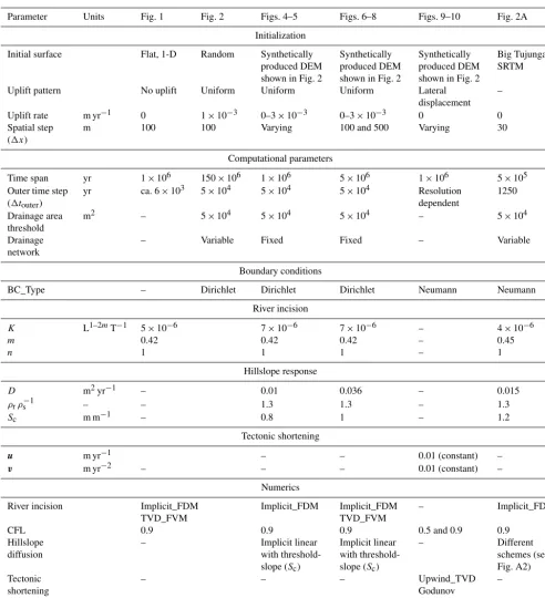
Table 1.Model parameters used for the TTLEM simulations.

Parameter Units Fig. 1 Fig. 2 Figs. 4–5 Figs. 6–8 Figs. 9–10 Fig. 2A

Initialization

Initial surface Flat, 1-D Random Synthetically

produced DEM shown in Fig. 2

Synthetically produced DEM shown in Fig. 2

Synthetically produced DEM shown in Fig. 2

Big Tujunga SRTM

Uplift pattern No uplift Uniform Uniform Uniform Lateral

displacement –

Uplift rate m yr−1 0 1×10−3 0–3×10−3 0–3×10−3 0 0

Spatial step (1x)

m 100 100 Varying 100 and 500 Varying 30

Computational parameters

Time span yr 1×106 150×106 1×106 5×106 1×106 5×105

Outer time step (1touter)

yr ca. 6×103 5×104 5×104 5×104 Resolution

dependent

1250

Drainage area threshold

m2 – 5×104 5×104 5×104 – 5×104

Drainage network

– Variable Fixed Fixed – Variable

Boundary conditions

BC_Type – Dirichlet Dirichlet Dirichlet Neumann Neumann

River incision

K L1–2mT−1 5×10−6 7×10−6 7×10−6 – 4×10−6

m 0.42 0.42 0.42 – 0.45

n 1 1 1 – 1

Hillslope response

D m2yr−1 – 0.01 0.036 – 0.015

ρrρs−1 – – 1.3 1.3 – 1.3

Sc m m−1 – 0.8 1 – 1.2

Tectonic shortening

u m yr−1 – – 0.01 (constant) –

v m yr−2 – – – 0.01 (constant) –

Numerics

River incision Implicit_FDM

TVD_FVM

Implicit_FDM Implicit_FDM

TVD_FVM

– Implicit_FDM

CFL 0.9 0.9 0.9 0.5 and 0.9 0.9

Hillslope diffusion

– Implicit linear

with threshold-slope (Sc)

Implicit linear with threshold-slope (Sc)

– Different

schemes (see Fig. A2) Tectonic

shortening

– – – Upwind_TVD

Godunov method

calling the algorithm repeatedly until all slope values are less than or equal toSc.

4 Impact of numerical methods

We investigate how numerical schemes implemented in TTLEM affect simulated landscape evolution. As we focus on evaluating the schemes’ performance, all simulations have synthetically generated landscapes as initial surfaces. Hence, our simulations are uncalibrated and results remain untested against an actual landscape: however, the chosen parameter values are within the range of previous studies (e.g., Gas-parini and Whipple, 2014; Whipple and Tucker, 1999). We distinguish between the effects on simulated river incision on the one hand and on simulated tectonic displacement on the other. To investigate the accuracy and implications of river incision methods, we compare the explicit TVD-FVM with the first-order implicit FDM and further differentiate be-tween the implicit FDM where no limitation is set on the time step and the implicit FDM where the CFL criterion limits the time step length. To investigate the accuracy and implications of river incision methods we compare an explicit first-order GM with the two-dimensional TVD-FVM.

4.1 River incision

4.1.1 One-dimensional river incision

The impact of numerical diffusion on propagating river pro-file knickpoints is most obvious in situations where an an-alytical solution is available. The first simulation illustrates such a situation, with an artificial river profile characterized by a major knickzone between 8 and 12 km from the river head (Fig. 1). We assume that the drainage area is increasing in proportion to the square of the distance and uplift equals zero. For this simplified configuration, an analytical solution for the SPL relies on the method of characteristics (Luke, 1972). Notwithstanding the relatively high spatial resolution of 100 m, the first-order implicit FDM suffers from consid-erable numerical diffusion when river incision is calculated over a time span of 1 My (Fig. 1). The TVD-FVM system-atically achieves a much higher accuracy over a wide range of spatial resolutions and parameter values (Campforts and Govers, 2015).

4.1.2 Drainage network

We assess the numerical accuracy of the entire drainage net-work with spatially and temporally constant values for all model parameter values (Table 1), assuming a fixed drainage network (see Sect. 3.3.2). We first create a steady-state ar-tificial landscape (Fig. 2) on a 50 km×100 km grid with a spatial resolution of 100 m that we initialize with uni-formly distributed random elevation values between 0 and 50 m (Movie S1 in the Supplement). Our simulation uses

Figure 1.Solution of the linear one-dimensional stream power law for a synthetic knickzone over a time span of 1 My. The analytical solution is obtained with the method of characteristics. The spatial resolution is 100 m. Table 1 lists other model parameter values.

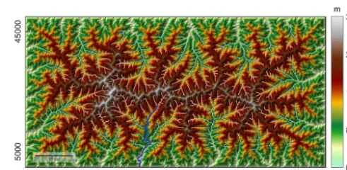
Figure 2.A synthetic steady-state landscape produced as the testing environment to verify and compare the different numerical schemes implemented in TTLEM. Model runtime was 150 My, while uplift rate was assumed to be spatially uniform over the area (block uplift) and fixed to 1 km My−1. Other model parameter values are listed in Table 1. Dynamic landscape evolution is presented in Movie S1. The gray lines indicate the drainage network for which the solution has been calculated analytically as a benchmark solution. The blue line indicates the river profile for which model results at different resolutions are plotted in Fig. 4.

Dirichlet boundary conditions and inserts a spatially and tem-porally uniform vertical uplift of 1 km My−1over a period of 150 My.1touteris set to 5×104years.

Figure 3.Uplift imposed on the steady-state landscape shown in Fig. 2 to investigate the impact of different numerical schemes.

domain covers 7950×15 950 cells), all model runs were exe-cuted on one computational node of the Flemish Super Clus-ter (VSC) using a single core (Broadwell, E5-2680v4) and 128 Gb RAM. We evaluate the numerical performance of the schemes and the impact of spatial resolution against an ana-lytical solution (slope patch method) for the entire drainage network represented by all cells exceeding 1 km2(Fig. 2).

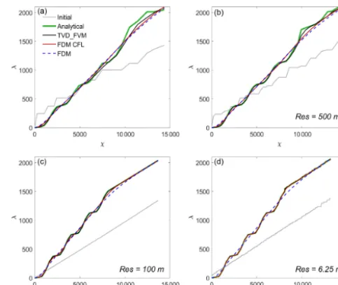
Figure 4 compares results obtained from the numerical methods and the analytical solution. The initial river profiles slightly differ depending on spatial resolution due to inter-polation of the steady-state artificial landscape with a spatial resolution of 100 m. The results show that TVD-FVM and implicit numerical solutions converge at increasing spatial resolutions. Where the time step of the implicit scheme is un-bounded by the CFL criterion, however, the solution deviates from those adhering to the CFL criterion. This illustrates that there is trade-off between numerical accuracy and numerical stability for an implicit scheme at long time steps. In addi-tion, an implicit scheme at high spatial resolution and large time steps fails to converge to an analytical solution because uplift is modeled as a discrete stepwise function rather than a continuous function (e.g., the sinusoidal uplift history used here) that inserts artificial shocks in the solution.

The TVD-FVM is consistently more accurate than the plicit methods at all spatial resolutions, although the im-plicit FDM (CFL < 1) approaches the high accuracy of the TVD-FVM at very high resolutions (6.25 m) (Fig. 5a). At lower spatial resolutions (> 10 m) the numerical accuracy of the TVD-FVM is significantly higher compared to the ac-curacy obtained with the implicit methods at the cost of a slightly increased additional computation time. To achieve the same numerical accuracy as the TVD-FVM at 500 m spatial resolution (RMSE=18.17, model runtime=2.89 s), the implicit method (CFL < 1) would need to be evaluated at 150 m, which would take 12 times longer (model run-time=36 s) (Fig. 5b).

4.1.3 River incision and catchment-wide erosion rates We hypothesize that the diffusive nature of commonly ap-plied first-order FDMs is not restricted to the simulation of river longitudinal profiles but has systematic consequences for other measures derived from LEM simulations. Such measures include catchment-wide erosion rates that

consti-Figure 4.Comparison between different modeled resolutions for the river profile indicated in blue in Fig. 2. The green line is the analytical “true” solution, obtained with the slope patch method of Royden and Perron (2013). The full red line represents the first-order accurate implicit solution when the CFL < 1, and the dotted blue line represents the first-order accurate implicit solution when the time step is left free. The implicit solutions where CFL < 1 are simulated with a time step equal to the time step used for the TVD-FVM.

Figure 5. (a) Performance of the different numerical schemes where the RMSE is calculated between the analytical and numer-ical methods.(b)CPU time required to perform the model runs at the indicated resolutions.

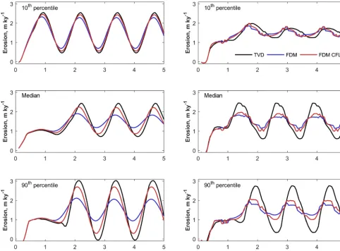
Figure 6.Temporal variation in simulated catchment-wide erosion rates using different numerical methods to simulate river incision. The black lines represent simulations where a flux-limiting TVD-FVM is used, the blue lines represent the first-order accurate implicit FDM without constraints on the time steps, and the red lines represent the first-order accurate FDM with an inner time step calculated with the CFL criterion.(a)Simulations performed at a spatial resolution of 100 m.(b)Simulations performed at a spatial resolution of 500 m. Here, a median filter with a window of three time steps is applied to the simulated erosion rates to eliminate spikes that might occur at low resolutions.

FDM without time step limitation, implicit FDM with time step limitation (CFL condition applied) and TVD-FVM) to simulate river incision. The maximum length of1tinneris set

to 3×103yr for all schemes to ensure that the implicit method converges at higher resolutions too (see Sect. 4.1.2). Hills-lope response is simulated using a linear diffusion scheme in combination with a threshold slope (Sc, see Fig. A2).

We compare differences in simulated erosion rates by ran-domly selecting > 200 catchments with drainage areas rang-ing between 1 and 50 km2(Fig. 7). We calculate the erosion rates for each time step by subtracting the elevation grid in the previous time step from the updated, current elevation grid. The sum of elevation differences within each catchment refers to the catchment-wide erosion rate integrated over the time step length. For each catchment, we then derive the difference between erosion rates calculated by the different numerical schemes and summarize them using the RMSE

statistics (OTVD−FDM):

OTVD−FDM=

s Pn

i=1 εi,TVD−εi,FDM2

nb1t

, (22)

whereεi,TVDandεi,FDMrefer to the catchment-wide erosion

rates simulated with the TVD-FVM and FDM, respectively, to simulate river incision, and nb1t is the total number of discrete time steps of the simulated erosion record.

We rank the catchments in increasing order ofOTVD−FDM

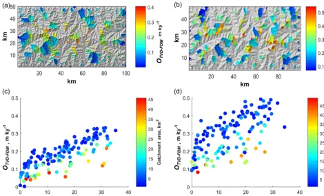
Figure 7.Spatial variation of differences between simulated erosion rates calculated with a flux-limiting TVD-FVM for simulating river incision and a first-order accurate implicit FDM. Here, we compare methods that are both run with an inner time step constrained with the CFL criterion (see text).OTVD−FDMis thus calculated between the black and red lines from Fig. 6. The left column represents simulations run at a spatial resolution of 100 m, the right column at 500 m.(a, b)Location of the randomly selected catchments with an area > 1 and < 50 km2. Colors refer to theOTVD−FDMbetween the two simulations.(c, d)Differences between the schemes increase with increasing distance from the river outlets and are inversely correlated with the catchment area.

For most catchments, we detect differences in catchment-wide erosion rates between the three numerical methods at a spatial resolution of 100 m. Generally, the amplitude of the response to a tectonic uplift pulse increases when us-ing TVD-FVM: the use of a first-order implicit FDM with-out time step restriction results in a much smoother response in comparison to the TVD-FVM. The variations in response amplitude are significant: the majority of the catchments record amplitude reductions by more than 50 % when mod-eled with the implicit FDM without time step restriction. Time step restriction (and thereby sacrificing the main ad-vantage of the implicit FDM) significantly reduces numer-ical diffusion so that most catchments display an erosional response comparable to that simulated by the TVD-FVM. However, this is only true for simulations with a 100 m spa-tial resolution. The advantage of a time-step-restricted im-plicit FDM over a nonrestricted imim-plicit FDM disappears al-most completely for a coarser grid resolution of 500 m.

Figure 7 shows that erosion rates diverge between the dif-ferent methods with increasing distance to the outlet of the main river, while they are similar for larger catchments. A smaller effect of the numerical scheme on large catchment

areas may partly arise from stronger averaging of local vari-ations in catchment erosion rates. In addition, catchments at a large distance from the outlet – and thus likely with smaller catchment areas – will experience upstream migrating knick-points only after several model time steps. If catchments are far from the fault zone, knickpoints will then be significantly smoothed by a first-order accurate implicit FDM, which will ultimately affect the response of the catchment. Again, spa-tial resolution matters: a larger grid size not only results in larger differences on average but also in larger differences between small and large catchments (Fig. 7).

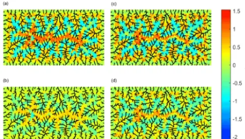
Figure 8.Spatial pattern of erosion rates during one model time step when simulating landscape evolution with the flux-limiting TVD-FVM vs. the first-order accurate implicit FDM.(a) Simula-tion at a resoluSimula-tion of 100 m where the time step of the implicit method is not constrained.(b)Simulation at a resolution of 100 m where the time step of the implicit method is constrained with the CFL criterion.(c)Simulation at a resolution of 500 m where the time step of the implicit method is not constrained.(d)Simulation at a resolution of 500 m where the time step of the implicit method is constrained with the CFL criterion.

4.2 Tectonic displacement

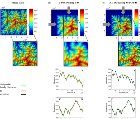
We test the performance of the two-dimensional version of the flux-limiting TVD-FVM to simulate tectonic displace-ment. A synthetic DEM forms the initial surface for a sim-ulation of a constant lateral tectonic displacement with nei-ther fluvial incision nor hillslope diffusion. Theoretically, this should result in a laterally displaced landscape that, apart from this displacement, remains unchanged in comparison to the initial state. We compare the flux-limiting TVD-FVM with a first-order accurate upwind GM simulating a tectonic displacement in two directions (u=v=10 mm yr−1) over a time span of 1 My. Figure 9 illustrates that the explicit GM strongly smooths the resulting DEM whereas the two-dimensional TVD-FVM scheme produces a DEM that is very similar to the initial DEM, with reduced amounts of numeri-cal diffusion.

In order to quantify the amount of numerical diffusion (DN

[L2yr−1]) introduced by the GM and the TVD-FVM method, we test a range of different model configurations and calcu-late the numerical diffusivity,DN, corresponding to the

ob-served smoothing.DNis the diffusivity required to transform

the initial DEM (DEMini) to the final DEMs produced at the

end of the simulations (DEMfint). The optimum amount of

diffusion is determined by minimizing the misfit functionH with a sequential quadratic programming method (Nocedal and Wright, 1999).His given by

H=

v u u u u t

nbpx

P

px=1

(DEMini−DEMfint)2

nbpx

, (23)

where nbpxis the number of pixels in the DEM.

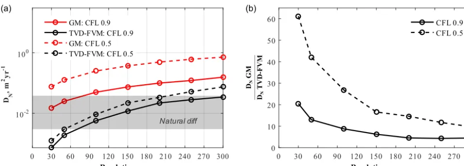
We find that numerical diffusivity of the GM exceeds com-monly used values of hillslope diffusivities as soon as spa-tial resolution exceeds 90 m (Fig. 10a). The two-dimensional TVD-FVM decreases numerical diffusion by a factor of 5–60 compared to the GM (Fig. 10b). The accuracy increases for both schemes with increasing resolution and increasing CFL numbers. However, the gain in accuracy with increasing spa-tial resolution is higher for the TVD-FVM than for the GM. Our analysis shows that the explicit FDM performs best with a CFL criterion close to one where additional required itera-tions within a given time interval are at a minimum (Gulliver, 2007).

5 Discussion

Our analysis of numerical solvers focuses on three interre-lated issues: numerical accuracy, spatial resolution and com-putational efficiency. Adopting highly simplifying assump-tions allow us to benchmark the solvers against analytical solutions. Our focus is on testing an implicit, first-order ac-curate FDM against TVD-FVM. The implicit FDM has sev-eral desirable properties. It is unconditionally stable and tol-erates time step lengths exceeding those prescribed by the CFL criterion. LEMs are often run over time spans of mil-lions of years and the CFL criterion is dictated by a few grid cells with high upslope areas. Adopting an implicit scheme is therefore potentially interesting since it allows the decrease of the computation time while enabling simulations at high spatial resolutions. Our results, however, show that this ma-jor advantage vanishes if the aim of a LEM simulation is to capture transiency correctly. For CFL > 1 the implicit FDM introduces significant numerical smearing, and for CFL1, the approach tends to insert an artificial shock wave of uplift because gradual uplift is approximated by a step function if time steps are (very) large.

Wil-Figure 9.Impact of numerical schemes when simulating horizontal shortening on a fixed grid. The simulations are performed at a spatial resolution of 50 m and a CFL of 0.5.(a)Extract from synthetically produced DEM from Fig. 2.(b)Horizontal shortening in two directions simulated with a two-dimensional explicit first-order GM. The green lines represent transects of the theoretically unchanged topography after lateral displacement. The red lines represent transects of the topography produced with the GM.(c)Horizontal shortening in two directions simulated with a two-dimensional explicit flux-limiting TVD-FVM (represented by black lines).

lett, 2013), it has severe shortcomings when simulating tran-sient landscape evolution caused by knickpoint propagation in detachment-limited erosional basins. These shortcomings can, to a large extent, be avoided by using a TVD-FVM.

We also show that the impact of the numerical scheme used to simulate river incision is not limited to river pro-file development alone. Hillslopes adjust to local base level changes dictated by river incision. Hillslope denudation rates must therefore – at least partly – reflect the geometry and dy-namics of a knickpoint and will respond differently to a dif-fuse signal that is the result of relatively slow, continuous up-lift on the one hand and sharp discontinuity caused by a rapid base-level drop of major fault activity on the other hand. Our

(a)

D N

,

m

2 y

r

-1

0 30 60 90 120 150 180 210 240 270 300

10-2 100

Natural diff

GM: CFL 0.9 TVD-FVM: CFL 0.9 GM: CFL 0.5 TVD-FVM: CFL 0.5

0 30 60 90 120 150 180 210 240 270 300

0 10 20 30 40 50

60 _{CFL 0.9}

CFL 0.5

DN

GM

DN

TVD-FVM

Resolution, m Resolution, m

Figure 10.(a)Amount of numerical diffusion (DN) introduced in the system when simulating lateral tectonic displacement in two directions as a function of raster resolution. The gray zone indicates the range of naturally observed diffusion rates.(b)The ratio between the amount of numerical diffusion for the first-order GM vs. the flux-limiting TVD-FVM.

far away from the base level since smoothing increases with time and knickpoint migration distance.

One might question the significance and necessity of nu-merical schemes that avoid diffusion of retreating knick-points. Given the many assumptions and uncertainties that underlie many LEMs, numerical accuracy may seem like a problem of lesser importance. We argue that the simulations presented in this paper show that this is not the case and that it is indeed critical to simulate knickpoint retreat as accu-rately as possible. However, our analysis does not cover all situations wherein the accurate simulation of knickzones is important. Simulation of sharp knickpoints is also required in geomorphological and lithological settings where knick-point retreat is caused by rock toppling, possibly triggered during extreme flood events (Baynes et al., 2015; Lamb et al., 2014; Mackey et al., 2014). Similarly, glacial incision of-ten creates hanging valleys that are reshaped by migrating fluvial knickpoints after glacial retreat (Valla et al., 2010). In all of these cases simulation tools with a minimum of nu-merical diffusion are required to correctly quantify natural knickpoint diffusion and to study the underlying processes.

First-order numerical methods also inadequately simulate lateral tectonic displacement on a regular grid. The amount of numerical diffusion that is introduced by these methods will, in many cases, exceed natural diffusion rates, thus mak-ing accurate simulation of hillslope development impossi-ble. A two-dimensional variant of the TVD-FVM reduces the amount of numerical diffusion to values well below nat-ural diffusivity values, an effect that is especially apparent at high spatial resolutions. The two-dimensional TVD-FVM thus allows the accurate modeling of this process, which sig-nificantly impacts the evolution of topography and river net-works (Willett, 1999), using a fixed grid. This was hitherto only possible with flexible spatial discretization schemes.

Although most LEMs use first-order accurate discretiza-tion schemes (Valters, 2016), the problem of numerical dif-fusion has been discussed in the broader geophysical com-munity (Durran, 2010; Gerya, 2010). An alternative fam-ily of shock-capturing Eulerian methods are MPDATA ad-vection schemes (Jaruga et al., 2015). These schemes are based on a two-step approach in which the solution is first approximated with a first-order upwind numerical scheme and then corrected by adding an anti-diffusion term (Pel-letier, 2008). However, contrary to the TVD-FVM, the stan-dard MPDATA scheme (Smolarkiewicz, 1983) is not mono-tonicity preserving (i.e., it is not TVD). Instead, MPDATA introduces dispersive oscillations in the solution if combined with a source term (such as uplift) in the equation (Durran, 2010). Adding limiters to the solution of the anti-diffusive step (Smolarkiewicz and Grabowski, 1990) renders the MP-DATA scheme oscillation free (Jaruga et al., 2015). However, by adding this additional correction, the method approaches the numerical nature of the TVD-FVM, which does not re-quire further adjustments in any case.

duces the shortcomings of rectangular grids while facilitating straightforward processing of model input and output.

6 Conclusion

Despite the growing interest in the development and use of LEMs, accuracy assessment of the numerical methods has received little attention. First-order accurate FDMs are the most commonly applied numerical methods. However, they introduce numerical diffusion and artificially smooth discontinuities that are inherent in transient landscapes. To overcome this problem, we developed the TVD-FVM. The TVD-FVM solves river incision more accurately than the first-order accurate FDMs with significant influences on the geometry of modeled river profiles and implications for catchment-wide erosion rates. Errors due to numerical dif-fusion depend on the spatial and temporal resolution as well as on the position of the catchment in the landscape. In ad-dition, we introduce a two-dimensional version of the TVD-FVM that allows the simulation of lateral tectonic displace-ment with low numerical diffusion on a fixed computational domain. Our new numerical techniques are implemented in the open-access raster-based Landscape Evolution Model (TTLEM) contained within TopoToolbox. Together with nu-merical implementations of common hillslope process

mod-limited to uplifting, fluvially eroding landscapes. Further de-velopment will integrate other processes (e.g., glacial ero-sion) as well as the explicit routing of sediment through the landscape.

7 Code and data availability

Appendix A

A1 Model structure

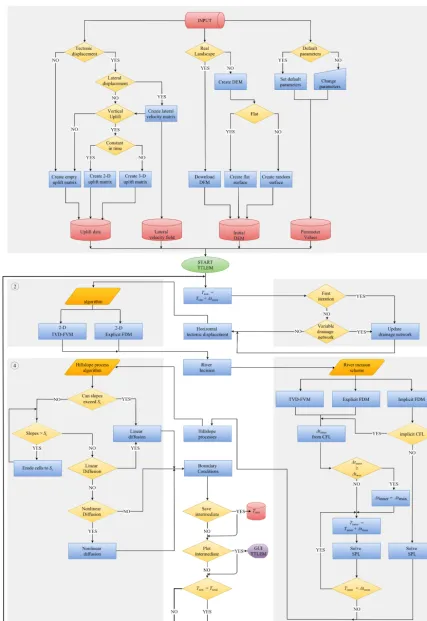
The model architecture of TTLEM is illustrated in Fig. A1.

A2 Hillslope processes

We illustrate the impact of different hillslope process mod-els on simulated landscape evolution using a 30 m resolution DEM of the Big Tujunga region in California as an example (Fig. A2). TTLEM allows the simulation of hillslope pro-cesses assuming (non)-linear slope-dependent diffusion with the consideration of a threshold hillslope. Figure A2 illus-trates how different hillslope process algorithms affect the evolution of hillslopes in the Big Tujunga region, Califor-nia (Fig. A2a). We assume no tectonic displacement and use standard parameter values for river incision and hillslope

dif-fusion (Table 1) and a threshold slope (Sc) of 1.2 (m m−1)

Competing interests. The authors declare that they have no con-flict of interest.

Acknowledgement. This work was motivated by the meeting

“Landscape evolution modeling – bridging the gap between field evidence and numerical models” in Hannover, 21–23 October 2015, which was organized by the FACSIMILE network and funded by the Volkswagen Foundation. Additional support comes from the Belgian Science Policy Office in the framework of the Interuniversity Attraction Pole project (P7/24): SOGLO – The soil system under global change. Numerical simulations were performed in the MATLAB environment (2015b) using numerical schemes as referred to in the text. Computational resources and services used to evaluate model performance were provided by the VSC (Flemish Supercomputer Center), managed by the Research Foundation – Flanders (FWO) in partnership with the five Flemish university associations. We are grateful to the IDYST group of the University of Lausanne and in particular Frédéric Herman and Aleksandar Licul for inspiring discussions on numerical methods and Nadja Stalder for the figure design. We further thank Taylor Perron for sharing his source code. We also thank the two anonymous reviewers and the editor for constructive feedback that improved the paper.

Edited by: J. Braun

Reviewed by: two anonymous referees

References

Andrews, D. J. and Bucknam, R. C.: Fitting degradation of shore-line scarps by a nonshore-linear diffusion model, J. Geophys. Res., 92, 12857, doi:10.1029/JB092iB12p12857, 1987.

Baynes, E. R. C., Attal, M., Niedermann, S., Kirstein, L. A., Dugmore, A. J., and Naylor, M.: Erosion during ex-treme flood events dominates Holocene canyon evolution in northeast Iceland, P. Natl. Acad. Sci., 112, 2355–2360, doi:10.1073/pnas.1415443112, 2015.

Blöthe, J. H., Korup, O., and Schwanghart, W.: Large landslides lie low: Excess topography in the Himalaya-Karakoram ranges, Geology, 43, 523–526, doi:10.1130/G36527.1, 2015.

Braun, J. and Sambridge, M.: Modelling landscape evolution on geological time scales: A new method based on irregular spa-tial discretization, Basin Res., 9, 27–52, doi:10.1046/j.1365-2117.1997.00030.x, 1997.

Braun, J. and Willett, S. D.: A very efficientO(n), implicit and par-allel method to solve the stream power equation governing flu-vial incision and landscape evolution, Geomorphology, 180–181, 170–179, doi:10.1016/j.geomorph.2012.10.008, 2013.

Burbank, D. W., Leland, J., Fielding, E., Anderson, R. S., Brozovic, N., Reid, M. R., and Duncan, C.: Bedrock incision, rock uplift and threshold hillslopes in the northwestern Himalayas, Nature, 379, 505–510, doi:10.1038/379505a0, 1996.

Campforts, B., Vanacker, V., Vanderborght, J., Baken, S., Smolders, E., and Govers, G.: Simulating the mobility of meteoric 10Be in the landscape through a coupled soil-hillslope model (Be2D), Earth Planet. Sc. Lett., 439, 143–157, doi:10.1016/j.epsl.2016.01.017, 2016a.

Campforts, B., Schwanghart, W., and Govers, G.: TTLEM – TopoToolbox Landscape Evolution: Synthetic model run, doi:10.5446/19197, 2016b.

Campforts, B., Schwanghart, W., and Govers, G.: TTLEM – Topo-Toolbox Landscape Evolution: Spatially and temporally variable tectonic configuration, doi:10.5446/19196, 2016c.

Croissant, T. and Braun, J.: Constraining the stream power law: a novel approach combining a landscape evolution model and an inversion method, Earth Surf. Dynam., 2, 155–166, doi:10.5194/esurf-2-155-2014, 2014.

Culling, W. E. H.: Soil Creep and the Development of Hillside Slopes, J. Geol., 71, 127–161, doi:10.1086/626891, 1963. DiBiase, R. A. and Whipple, K. X.: The influence of erosion

thresh-olds and runoff variability on the relationships among topog-raphy, climate, and erosion rate, J. Geophys. Res.-Earth, 116, F04036, doi:10.1029/2011JF002095, 2011.

DiBiase, R. A., Whipple, K. X., Heimsath, A. M., and Ouimet, W. B.: Landscape form and millennial erosion rates in the San Gabriel Mountains, CA, Earth Planet. Sc. Lett., 289, 134–144, doi:10.1016/j.epsl.2009.10.036, 2010.

Dietrich, W. E., Bellugi, D. G., Sklar, L. S., Stock, J. D., Heim-sath, A. M., and Roering, J. J.: Geomorphic Transport Laws for Predicting Landscape form and Dynamics, in: Prediction in Geomorphology, edited by: Wilcock, P. R. and Iverson, R. M., 103–132, American Geophysical Union, Washington, DC, USA, 2013.

Durran, D. R.: Numerical Methods for Fluid Dynamics, Springer New York, NY, USA, 2010.

Gasparini, N. M. and Whipple, K. X.: Diagnosing climatic and tec-tonic controls on topography: Eastern flank of the northern Boli-vian Andes, Lithosphere, 6, 230–250, doi:10.1130/L322.1, 2014. Gerya, T.: Introduction to Numerical Geodynamic Modelling,

Cam-bridge University Press, CamCam-bridge, UK, 2010.

Glotzbach, C.: Deriving rock uplift histories from data-driven inversion of river profiles, Geology, 43, 467–470, doi:10.1130/G36702.1, 2015.

Godunov, S. K.: A Finite Difference Method for the Computation of Discontinuous Solutions of the Equations of Fluid Dynamics, Math. USSR-Sbornik, 47, 271–306, 1959.

Goren, L., Willett, S. D., Herman, F., and Braun, J.: Coupled numerical-analytical approach to landscape evolution modeling, Earth Surf. Proc. Land., 39, 522–545, doi:10.1002/esp.3514, 2014.

Gulliver, J. S.: Introduction to Chemical Transport in the Environ-ment, Cambridge University Press, Cambridge, UK, 2007. Harten, A.: High resolution schemes for hyperbolic

Herman, F. and Braun, J.: Fluvial response to horizontal shortening and glaciations: A study in the Southern Alps of New Zealand, J. Geophys. Res., 111, F01008, doi:10.1029/2004JF000248, 2006. Hoke, G. D., Isacks, B. L., Jordan, T. E., Blanco, N., Tomlinson, A. J., and Ramezani, J.: Geomorphic evidence for post-10 Ma uplift of the western flank of the central Andes 18◦300–22◦S, Tectonics, 26, TC5021, doi:10.1029/2006TC002082, 2007. Howard, A. D.: A detachment-limited model of drainage

basin evolution, Water Resour. Res., 30, 2261–2285,

doi:10.1029/94WR00757, 1994.

Howard, A. D. and Kerby, G.: Channel changes in bad-lands, Geol. Soc. Am. Bull., 94, 739–752, doi:10.1130/0016-7606(1983)94<739:CCIB>2.0.CO;2, 1983.

Jaruga, A., Arabas, S., Jarecka, D., Pawlowska, H., Smolarkiewicz, P. K., and Waruszewski, M.: libmpdata++1.0: a library of paral-lel MPDATA solvers for systems of generalised transport equa-tions, Geosci. Model Dev., 8, 1005–1032, doi:10.5194/gmd-8-1005-2015, 2015.

Jungers, M. C., Bierman, P. R., Matmon, A., Nichols, K., Larsen, J., and Finkel, R.: Tracing hillslope sediment production and trans-port with in situ and meteoric10Be, J. Geophys. Res., 114, 1–16, doi:10.1029/2008JF001086, 2009.

Kirby, E. and Whipple, K.: Quantifying differential rock-uplift rates via stream profile analysis, Geology, 29, 415–418, doi:10.1130/0091-7613(2001)029<0415:QDRURV>2.0.CO;2, 2001.

Korup, O.: Rock-slope failure and the river long profile, Geology, 34, 45–48, doi:10.1130/G21959.1, 2006.

Lague, D.: The stream power river incision model: evidence, theory and beyond, Earth Surf. Proc. Land., 39, 38–61, doi:10.1002/esp.3462, 2014.

Lamb, M. P., Mackey, B. H., and Farley, K. A.:

Amphitheater-headed canyons formed by megaflooding at Malad

Gorge, Idaho, P. Natl. Acad. Sci. USA, 111, 57–62,

doi:10.1073/pnas.1312251111, 2014.

Larsen, I. J. and Montgomery, D. R.: Landslide erosion cou-pled to tectonics and river incision, Nat. Geosci., 5, 468–473, doi:10.1038/ngeo1479, 2012.

Lax, P. and Wendroff, B.: Systems of conservation laws, Commun. Pur. Appl. Math., 13, 217–237, doi:10.1002/cpa.3160130205, 1960.

Luke, J. C.: Mathematical models for landform evolution, J. Geophys. Res., 77, 2460–2464, doi:10.1029/JB077i014p02460, 1972.

Mackey, B. H., Scheingross, J. S., Lamb, M. P., and Farley, K. A.: Knickpoint formation, rapid propagation, and landscape re-sponse following coastal cliff retreat at the last interglacial sea-level highstand: Kaua’i, Hawai’i, Geol. Soc. Am. Bull., 126, 925–942, doi:10.1130/B30930.1, 2014.

Moon, S., Shelef, E., and Hilley, G. E.: Recent topographic evolu-tion and erosion of the deglaciated Washington Cascades inferred from a stochastic landscape evolution model, J. Geophys. Res.-Earth, 120, 856–876, doi:10.1002/2014JF003387, 2015. Mudd, S. M.: Detection of transience in eroding landscapes, Earth

Surf. Proc. Land., 42, 24–41, doi:10.1002/esp.3923, 2016. Mudd, S. M., Attal, M., Milodowski, D. T., Grieve, S. W. D.,

and Valters, D. A.: A statistical framework to quantify spa-tial variation in channel gradients using the integral method of

channel profile analysis, J. Geophys. Res.-Earth, 119, 138–152, doi:10.1002/2013JF002981, 2014.

Nocedal, J. and Wright, S. J.: Numerical Optimization, Springer, New York, USA, 1999.

Pelletier, J. D.: Quantitative Modeling of Earth Surface Processes, Cambridge University Press, Cambridge, UK, 2008.

Pelletier, J. D.: Minimizing the grid-resolution dependence of flow-routing algorithms for geomorphic applications, Geomorphol-ogy, 122, 91–98, doi:10.1016/j.geomorph.2010.06.001, 2010.

Perron, J. T.: Numerical methods for nonlinear

hills-lope transport laws, J. Geophys. Res., 116, F02021,

doi:10.1029/2010JF001801, 2011.

Phillips, J. D., Schwanghart, W., and Heckmann, T.: Graph theory in the geosciences, Earth-Sci. Rev., 143, 147–160, doi:10.1016/j.earscirev.2015.02.002, 2015.

Roering, J. J., Kirchner, J. W., and Dietrich, W. E.: Evidence for nonlinear, diffusive sediment transport on hillslopes and impli-cations for landscape morphology, Water Resour. Res., 35, 853– 870, doi:10.1029/1998WR900090, 1999.

Royden, L. and Perron, T. J.: Solutions of the stream power equa-tion and applicaequa-tion to the evoluequa-tion of river longitudinal profiles, J. Geophys. Res.-Earth, 118, 497–518, doi:10.1002/jgrf.20031, 2013.

Schwanghart, W. and Kuhn, N. J.: TopoToolbox: A set of Matlab functions for topographic analysis, Environ. Model. Softw., 25, 770–781, doi:10.1016/j.envsoft.2009.12.002, 2010.

Schwanghart, W. and Scherler, D.: Short Communication: Topo-Toolbox 2 – MATLAB-based software for topographic analysis and modeling in Earth surface sciences, Earth Surf. Dynam., 2, 1–7, doi:10.5194/esurf-2-1-2014, 2014.

Schwanghart, W., Groom, G., Kuhn, N. J., and Heckrath, G.: Flow network derivation from a high resolution DEM in a low re-lief, agrarian landscape, Earth Surf. Proc. Land., 38, 1576–1586, doi:10.1002/esp.3452, 2013.

Seidl, M. and Dietrich, W.: The problem of channel erosion into bedrock (Supplement), Catena, 23, 101–104, 1992.

Smolarkiewicz, P. K.: A Simple Positive Definite

Ad-vection Scheme with Small Implicit Diffusion, Mon.

Weather Rev., 111, 479–486,

doi:10.1175/1520-0493(1983)111<0479:ASPDAS>2.0.CO;2, 1983.

Smolarkiewicz, P. K. and Grabowski, W. W.: The multidimen-sional positive definite advection transport algorithm: nonoscil-latory option, J. Comput. Phys., 86, 355–375, doi:10.1016/0021-9991(90)90105-A, 1990.

Soille, P., Vogt, J., and Colombo, R.: Carving and adaptive drainage enforcement of grid digital elevation models, Water Resour. Res., 39, 1366, doi:10.1029/2002WR001879, 2003.

Stock, J. D. and Montgomery, D. R.: Geologic constraints on bedrock river incision using the stream power law, J. Geophys. Res., 104, 4983, doi:10.1029/98JB02139, 1999.

Toro, E. F.: Riemann solvers and numerical methods for fluid dy-namics – A Practical Introduction, Springer, New York, USA, 2009.

Vanacker, V., von Blanckenburg, F., Govers, G., Molina, A., Camp-forts, B., and Kubik, P. W.: Transient river response, captured by channel steepness and its concavity, Geomorphology, 228, 234– 243, doi:10.1016/j.geomorph.2014.09.013, 2015.

van Leer, B.: Towards the Ultimate Conservative

Dif-ference Scheme, J. Comput. Phys., 135, 229–248,

doi:10.1006/jcph.1997.5704, 1997.

West, N., Kirby, E., Bierman, P., Slingerland, R., Ma, L., Rood, D., and Brantley, S.: Regolith production and transport at the Susquehanna Shale Hills Critical Zone Observatory, Part 2: In-sights from meteoric10Be, J. Geophys. Res.-Earth, 118, 1877– 1896, doi:10.1002/jgrf.20121, 2013.

doi:10.1029/1999JB900120, 1999.

Whittaker, A. C., Cowie, P. A., Attal, M., Tucker, G. E., and Roberts, G. P.: Contrasting transient and steady-state rivers cross-ing active normal faults: New field observations from the central apennines, Italy, Basin Res., 19, 529–556, doi:10.1111/j.1365-2117.2007.00337.x, 2007.

Willett, S. D.: Orogeny and orography: The effects of erosion on the structure of mountain belts, J. Geophys. Res.-Sol. Ea., 104, 28957–28981, doi:10.1029/1999JB900248, 1999.