www.nonlin-processes-geophys.net/16/503/2009/ © Author(s) 2009. This work is distributed under the Creative Commons Attribution 3.0 License.
Nonlinear Processes
in Geophysics
Characterization of peak flow events with local singularity method
Q. Cheng1,2, L. Li2, and L. Wang2
1State Key Laboratory of Geological Processes and Mineral Resources, China University of Geosciences,
Wuhan, Beijing, China
2Department of Earth and Space Science and Engineering, Department of Geography, York University, Toronto,
Ontario M3J1P3, Canada
Received: 13 February 2008 – Revised: 17 June 2009 – Accepted: 14 July 2009 – Published: 22 July 2009
Abstract. Three methods, return period, power-law fre-quency plot (concentration-area) and local singularity in-dex, are introduced in the paper for characterizing peak flow events from river flow data for the past 100 years from 1900 to 2000 recorded at 25 selected gauging stations on rivers in the Oak Ridges Moraine (ORM) area, Canada. First a tra-ditional method, return period, was applied to the maximum annual river flow data. Whereas the Pearson III distribution generally fits the values, a power-law frequency plot (C-A) on the basis of self-similarity principle provides an effective mean for distinguishing “extremely” large flow events from the regular flow events. While the latter show a power-law distribution, about 10 large flow events manifest departure from the power-law distribution and these flow events can be classified into a separate group most of which are related to flood events. It is shown that the relation between the average water releases over a time period after flow peak and the time duration may follow a power-law distribution. The exponent of the power-law or singularity index estimated from this power-law relation may be used to characterize non-linearity of peak flow recessions. Viewing large peak flow events or floods as singular processes can anticipate the application of power-law models not only for characterizing the frequency distribution of peak flow events, for example, power-law re-lation between the number and size of floods, but also for describing local singularity of processes such as power-law relation between the amount of water released versus releas-ing time. With the introduction and validation of sreleas-ingular- singular-ity of peak flow events, alternative power-law models can be used to depict the recession property as well as other types of non-linear properties.
Correspondence to: Q. Cheng ([email protected])
1 Introduction
Humankind has always been faced with water resource prob-lems – floods and droughts. Flood disasters have been more devastating in terms of deaths, suffering, and economical damages are concerned, versus other natural hazards e.g., earthquakes, volcanoes, and wild fires etc. (Kundzewicz et al., 1993). Despite the progress in science and technology, humans are still vulnerable to extreme hydrological events. The losses increase due to the continuing development of costly infrastructure, rise in population density, and decrease of buffering capacities such as deforestation, urbanization, and draining wetlands. Despite heavy expenditures on both, structural and non-structural measures of flood and drought control, extreme hydrological events continue to present a hazard in developed and developing parts of the world. Un-derstanding floods and droughts, their mechanisms, charac-teristics, and regularities is of crucial importance for water assessments, water allocation, design and management of water resource systems.
distribution with algebraic tails with exponent−qD, which is related to multifractal phase transition and self-organized criticality (SOC) (Bak et al., 1987). The extreme events might cause divergence property of statistical moments with spatial scaling (Lovejoy and Schertzer, 1995). Similar behav-ior was found by Turcotte and Greene (1993) in river flows. These works have provided framework for identifying statis-tical property of extreme events. From a pracstatis-tical point of view, however, one needs sophisticated software and good knowledge of multifractal modeling in order to use these methods to characterize the properties of extreme events and to appreciate the effectiveness of these methods. Further research on separation of regular and extreme events is re-quired to develop guidelines for an optimal choice of thresh-old in consideration of both physical and statistical charac-teristics of extreme hydrologic processes (Nguyen, 2001). This paper explores some simple methods for characteriz-ing extreme river flow events. Instead of “extreme nature” of events, we will consider “singularity” of the events. Singular geo-processes including physical, chemical and biological processes may result in anomalous amounts of energy release or mass accumulation or matter concentration that, generally, are confined to narrow intervals in space or time (Cheng, 2007a). It has been found that the end products of these non-linear processes including cloud formation (Schertzer and Lovejoy, 1987), rainfall (Veneziano, 2002), hurricanes (Sornette, 2004), flooding (Malamud, Turcotte and Barton, 1996), landslides (Malamud et al., 2004), earthquakes (Tur-cotte, 1997), mineral deposits (Agterberg, 1995) and miner-alization (Cheng, 2007a) have in common that they can be modeled as fractals or multifractals. Total amount of ore and metals in hydrothermal ore deposits often have Pareto tails (Turcotte, 1997). Hydrothermal mineral deposits also can exhibit non-linear features for ore-mineral and associated toxic element concentration values in rock and related sur-face media such as water, soil, stream sediment, till, humus and vegetation (Cheng, 2007a; Cheng and Agterberg, 2009). As a singular process, extreme river flow or floods have been extensively studied from non-linear processes point of view. Several interesting characteristics of river flow fluctuations were reported: the river flow series have power-law tails in the probability distribution (Murdock and Gulliver, 1993; Turcotte and Greene, 1993; Movahed and Hermanis, 2008), which will be confirmed with the data used in the current pa-per; river flow series are long-range correlated (Hurst, 1951); River flow series are multifractals (Lovejoy and Schertzer, 1995). Gupta (2004), Gupta and Waymire (1990) and Gupta et al. (1996) have systematically investigated the statistical self-similarity or scale invariance in the spatial variability of rainfall, channel network structures and floods. This frame-work provides foundations for solving the global problem of prediction of floods from ungauged and poorly gauged basins (Gupta, 2004).
From singularity point of view, singular events are usu-ally rare but not necessarily unique, profound, or significant
in terms of their impacts, effects, or outcomes. These types of events are relatively rare due to their abnormality and in-volving long processes of energy and material accumulation. Whether these processes cause significant impact depend on where and when they happen. As a matter of fact, singular processes affect human society in two sides: providing re-sources and causing hazards. On the one hand, with proper technology the energy released or material accumulated dur-ing the sdur-ingular processes could be utilized as resources for human society development, for example mineral resources, on the other hand, the explosive energy release and anoma-lous concentration of materials including toxic materials can also cause hazardous impacts on ecological and human sys-tems. This paper explores non-linear modeling techniques to identify and characterize singular hydrological events – floods from historical data collected from river flow gaug-ing stations. It will introduce three methods: return period, frequency plot (C-A method) and singularity index for iden-tification and for characterization of singular events – floods. The first method is the traditional and used by hydrologists for quantifying an extreme hydrological event by estimating how long such an event happens likely. The second method is also commonly used for characterizing distribution of hy-drologic events and for separating “regular” from “extreme” events (Cheng et al., 1994). The third method was proposed and applied for identifying and characterizing local singular-ities observed in the complex maps used in mineral explo-ration (Cheng, 2007a; Cheng and Agterberg, 2009). These three methods were applied to the river flow data collected from 1900–2000 at 25 river gauging stations in the Oak Ridges Moraine (ORM), southern Ontario, Canada.
2 Study area and data
The study area of the Oak Ridges Moraine (ORM) is located in southern Ontario, Canada. This is one of the most devel-oped areas in Canada. The moraine is characterized by its rolling hills and river valleys extending 160 km from the Ni-agara Escarpment to Rice Lake, and was formed 12 000 years ago by advancing and retreating glaciers. The moraine con-tains the headwaters of 65 river systems and has a wide diver-sity of streams, woodlands, wetlands, kettle lakes, kettle bogs and significant flora and fauna. It is one of the last remaining continuous green corridors in southern Ontario containing 30 per cent forested area. A comprehensive introduction about hydrology of southern Ontario can be found in the Hydroge-ology of Ontario Report (Singer et al., 2003). The moraine’s sands and gravel deposits absorb rain and snow melt. The underground water is then stored in layers of sand and gravel (aquifers), filtered and slowly released as cool fresh water to the 65 rivers and streams flowing north into Lakes Simcoe and Scugog and south into Lake Ontario.
includes deep winter snow, heavy spring and summer thun-derstorms, and, sometimes, lengthy summer dry spells. The temperature is moderate most of the time and, annually, there is approximately 600 to 1000 mm of precipitation including snow in winter season and rainfall in other seasons across the ORM area (Brown et al., 1968). Snowfall mainly in De-cember to March accounts for about 15 per cent of the to-tal annual precipitation. In the summer, widespread daily-long rainfalls are rare. Instead, showery precipitation is the general rule. This frequently results in precipitation varying widely from place to place. In addition, this kind of precipi-tation may come as short but intense downpours that quickly run into drains and streams. A thunderstorm that results in 20 or 30 mm of rain in just one hour does little to relieve the moisture deficit that comes with a long period of dry weather (Brown et al., 1968; Singer et al., 2003).
On occasion, this area receives the effects of the remnants of a tropical storm or hurricane moving through the eastern part of the United States. Occurring from mid-summer to autumn, these systems may result in an all-day rainfall that can be quite heavy. Precipitation amounts from these sys-tems can also be somewhat variable over relatively short dis-tances. When Hurricane Hazel hit the area in October 1954, 181.6 mm of rain was recorded at Snelgrove station: how-ever, only 38.1 mm at Alton station just 22 km northwest of Snelgrove at the same time (Singer et al., 2003).
Land-use in the ORM area is largely rural, with forest and agricultural practices dominating the landscape although it includes the Greater Toronto Area that is a highly industrial-ized area. Increasing population and residential development in this area has led to residential development expanding into the rural areas. Land-use changes, primarily the build-ing of residential subdivisions, the construction of roads and the paving of parking lots, increase the imperviousness of the ground surface. Consequently, this surface runoff results in dramatic increases in wet weather flows of the headwater streams on the Moraine causing erosion and degradation of these fragile systems (STORM-Coalition, 1997).
Various modeling exercises conducted on the study area have demonstrated that runoff volumes observed at the river gauging stations in the drainage basin networks are highly correlated with the baseflow caused by ground water dis-charge, snow melting, direct flow caused by rainfall as well as the physical properties of drainage basins (Cheng et al., 2006). It has been found that the delay response of sur-face runoff (river peak flow) to heavy precipitation events varies across the study area depending on the physical prop-erties of drainage networks and stream systems such as the complexity of drainage basin boundaries, glacier sediment types, land-use types, and surface inclination (Ko and Cheng, 2004). It has been demonstrated that long-term persistency of river flow is related to the characteristics of drainage basins (Ko and Cheng, 2004; Cheng et al., 2006, 2008). The in-teraction between groundwater and surface runoff also has been investigated so that the influence of groundwater
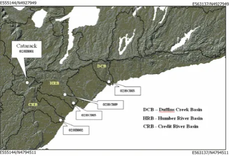
Figure 1. Shaded relief of the digital elevation model of the ORM (DEM data from Kenny, 1997). Lines represent the major basins of the area. White dots represent the locations of some river gauging stations. Labels in the boxes are the IDs of gauging stations.
1
Fig. 1. Shaded relief of the digital elevation model of the ORM (DEM data from Kenny, 1997). Lines represent the major basins of the area. White dots represent the locations of river gauging stations chosen for the study. Labels in the boxes are the IDs of gauging stations.
charge on river flow could be modeled (Cheng et al., 2001, 2006; Cheng, 2004). The conventional SCS method (Soil Conservation Service) of the US Department of Agriculture, Soil Conservation Service (1972) and IHACRES (Identifica-tion of Unit Hydrographs and Component Flows from Rain-fall, Evaporation, Stream flow data) developed by Jakeman et al. (1990), Jakeman and Hornberger (1993) and Jakeman et al. (1994) have been applied to predict annual runoff volume in the river system including ungauged basins from observed precipitation records (Cheng et al., 2004).
In order to identify and characterize flood events from the singularity point of view, we have selected 25 gauging sta-tions in the Oak Ridges Moraine (ORM) area (data from HYDAT CD-ROM User’s Manual, 1996). These stations have records of mean daily flow (m3/s) and daily rainfall data since 1900. The locations of the gauging stations are shown in Fig. 1 superimposed on a selected digital eleva-tion model (DEM) showing the landscape of the ORM area (Kenny, 1997). Daily flow data from these stations are used to calculate return period using Pearson III distribution. The same dataset were analyzed by C-A method for separating flood events from regular river flow events. The peak flow events identified by return period and C-A method were fur-ther analyzed by local singularity analysis.
3 Return period
detrimental impacts on ecosystems and human society than average climate conditions (Hengeveld, 2000). The identifi-cation and characterization of extreme hydrological events is one of the most important concerns of hydrologists.
Climatologists use a variety of statistical criteria to iden-tify extreme events (IPCC, 2001). Return period denotes a recurrence interval of defined hydrological events. It is a sta-tistical measure of how often an event of a certain size is likely to happen. Flood size can be treated as a random vari-able and the return period defined as the mean period of event reoccurrence. For example, a large flood event with 100-year return period likely reoccurs in 100 years but it does not nec-essarily happen again after exactly 100 years. For a proba-bility distribution of event sizeX,P(X≥x), estimated from a long series of events in unit of year, the return period of event with sizex can be calculated from the inverse of the probability of the event, or,
T = 1
P (X≥x) (1)
whereT is the return period in years, P(X≥x) is the prob-ability of the event with value ofX≥x. This equation in-dicates that each year the probability of an event with size abovexisP (X≥x). Therefore, in order to have an event re-occur it needs to have a period ofT years so thatT P=1, that isT=1/P.
The Pearson Type III, or Gamma distribution describes the probability of occurrence of an event as a Poisson process. When the population of events is very positively skewed, the data are fitted by Log Pearson Type III Distribution. This type of distribution is determined by three parameters that are related to the mean, variance and skewness of the dis-tribution. The Pearson Type III Distribution was originally applied in hydrology to describe the distribution of annual maximum discharge (Foster and Alden, 1924). The Log Pearson Type III Distribution is commonly used to calculate flood recurrences (Viessman and Lewis, 2003).
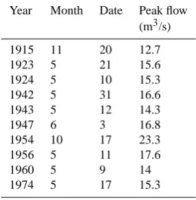
The values of maximum annual discharges recorded at all stations in the area over the past 100 years from 1900 to 2000 were fitted by Log Pearson Type III Distribution. Results show that Log Pearsontype III distribution generally fits the data although the values in the two tails show deviations from the model. From the Pearson type III curve one can derive the probability of any given discharge that, in turn, can be converted into an estimate of return period. For example, the flood events that occur on October 1954, May 1956, and June 1947 reached peak flows 23.3, 17.6, and 17.3 m3/s, respec-tively, then, from the curve we can estimate that the return periods should be 77, 30, and 29 years, respectively.
4 Power-law frequency distribution
Probability plot is a common way to plot river flow data and power-law tails have been reported by several authors (Mur-dock and Gulliver, 1993; Turcotte and Greene, 1993). It has
been reported that the background or regular and anomaly or extreme events may follow different distribution based on which one can separate these two populations (Cheng et al., 1994). As a matter of fact, many singular processes result in end products with fractal or multifractal distributions. Ex-amples include number and size distribution of earthquakes, landslides, forest fires, and floods (Turcotte, 2001). Power-law distribution has the unique property of scale invari-ance and self-similarity (generalized self-similarity in case of anisotropy scaling). Since power-law function can be eas-ily plotted as linear function on double log-scale, it is often intuitive to inspect whether values follow power-law distri-bution or self-similar distridistri-bution. Therefore, these types of plots can be applied to inspect and to separate populations based on distinct generalized self-similarities of populations. For example, a 2-D concentration-area fractal method (C-A) proposed for separating geo-anomalies from background on the basis of distinct power-law relations has been commonly used in exploration geochemistry for anomaly identification and environmental geochemistry for regional pollution pat-tern recognition (Cheng et al., 1994). This method is based on a relation associating concentration (or density) value (v) and the area (or accumulative number) within which concen-tration values are above a thresholdρ,(A(v≥ρ))as
A(v≥ρ)=Cρ−β (2)
Log (f)
Log [ND(>f)]
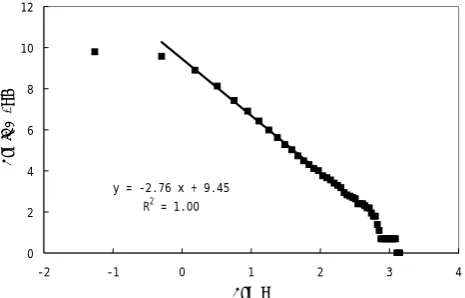
Figure 2 Log-log plot of number of days ND(≥f) against the flow rate (f) at Cataract
Station. Both axes are in natural logarithmic transformed scale.
1
Fig. 2. Log-log plot of number of days ND(≥f) against the flow
rate (f in m3/s) at Cataract Station. Both axes are in natural loga-rithmic transformed scale.
of days with flow data fail in each of these intervals were calculated and are shown in Table 1 and plotted on Fig. 2.
The frequency values of number of days versus flow data generally shows a linear trend on the log-log plot, although the values in the two tails clearly departure from the lin-ear trend. The main segment of the plot shows a linear relation between transformed number of days and log-transformed flow data log [ND(≥f)]=2.76 log (f)+9.45 with squared linear correlation coefficientR2=0.999. This ensures that the number of days and flow data follows the power-law relation ND(≥f)=12708f−2.76. From the plot one can see that 10 large flow points with flow discharge above 12 m3/s depart from the straight line and the actual events in this group are shown in Table 2. The plot in Fig. 2 may indicate that the main flow data except the 10 large flow data show a type of self-similarity. The differences between the distri-bution types of the main values and the large values might reflect different underlying processes or be due to errors in data recording. However, the data from most stations in the study area show similar characteristics and this may indi-cate that the difference is indeed due to different causes of large flow. Therefore, these large flow events can be iden-tified as a separate group of extreme flow events that differ from the main flow events which can be considered as reg-ular flow events. The extreme flow events might be due to extreme weather conditions as occurred, for example, when hurricane Hazel struck the Toronto area on 15 and 16 Octo-ber 1954 with great amounts of precipitation. For example, if the river discharge is beyond the river flow capacity, then flooding would occur and river flow recorded at the gaug-ing station could become less than what it would be without flooding. Although the causes of the scale break need further investigation, their identification already provides useful in-formation about these events. Later in this paper it will be shown that extreme flow events show strong local singular-ity that can be further characterized using local singularsingular-ity analysis.
0 0.5 1 1.5 2 2.5 3 3. Log Discharge
Log (Probability)
5
Figure 3 Frequency analyses of maximum annual peak flow from Cataract Station on
Credit River. Straight line segments are fitted by least square method. Log is natural log.
1
Fig. 3. Frequency analyses of maximum annual peak flow (m3/s)
from Cataract Station on Credit River. Straight line segments are fitted by least square method. Log is natural log.
Following the same principle, we can reconsider the an-nual maximum flow data previously fitted by log Pearson III function. The results are shown in Fig. 3 which shows three straight-line segments providing a good fit to the data with cutoff values that separate the maximum annual flow values into three distinct groups. The group on the far right side gives a cutoff value 14 according to which one can identify a group of large maximum annual flow values. The results are similar to those in Table 2 except for the event in 1915.
5 Singularity of peak flow
Table 1. Relationship between accumulative number of days with discharge (m3/s) above an threshold and the threshold calculated from flow data at the Catarack Station on Credit River.
Threshold Number Log Log Threshold Number Log Log
Discharge of Days Threshold Days Discharge of Days Threshold Days
0.28 17970 −1.26 9.80 12.25 14 2.51 2.64
0.74 14446 −0.30 9.58 12.71 11 2.54 2.40
1.20 7328 0.19 8.90 13.17 11 2.58 2.40
1.66 3391 0.51 8.13 13.63 11 2.61 2.40
2.12 1677 0.75 7.42 14.09 10 2.65 2.30
2.58 999 0.95 6.91 14.55 9 2.68 2.20
3.05 618 1.11 6.43 15.01 9 2.71 2.20
3.51 399 1.25 5.99 15.47 7 2.74 1.95
3.97 276 1.38 5.62 15.93 6 2.77 1.79
4.43 196 1.49 5.28 16.39 6 2.80 1.79
4.89 152 1.59 5.02 16.86 4 2.82 1.39
5.35 113 1.68 4.73 17.32 3 2.85 1.10
5.81 89 1.76 4.49 17.78 2 2.88 0.69
6.27 74 1.84 4.30 18.24 2 2.90 0.69
6.73 61 1.91 4.11 18.70 2 2.93 0.69
7.19 55 1.97 4.01 19.16 2 2.95 0.69
7.65 43 2.03 3.76 19.62 2 2.98 0.69
8.11 39 2.09 3.66 20.08 2 3.00 0.69
8.57 35 2.15 3.56 20.54 2 3.02 0.69
9.03 30 2.20 3.40 21.00 2 3.04 0.69
9.49 27 2.25 3.30 21.46 2 3.07 0.69
9.95 24 2.30 3.18 21.92 2 3.09 0.69
10.41 19 2.34 2.94 22.38 1 3.11 0.00
10.87 17 2.39 2.83 22.84 1 3.13 0.00
11.33 16 2.43 2.77 23.30 1 3.15 0.00
11.79 15 2.47 2.71
Table 2. Extreme flood events of cataract station.
Year Month Date Peak flow (m3/s)
1915 11 20 12.7
1923 5 21 15.6
1924 5 10 15.3
1942 5 31 16.6
1943 5 12 14.3
1947 6 3 16.8
1954 10 17 23.3
1956 5 11 17.6
1960 5 9 14
1974 5 17 15.3
as will be shown below. Considering the short time period between heavy rainfall and peak flow caused by this rainfall and the fact that there are not enough multiple daily flow data before the flow peak to conduct statistical analysis, here we will only use the flow series following the flow peak, i.e., for
recession flow only. Initial timet0 can be set the peak. To
avoid overlap of multiple peak flow, we further select flow series showing single peak and there was no significant rain-fall after the peak flow. AssumeQ1,Q2, . . . , andQnare the daily flow data available; these data usually are in descend-ing order. The average flow within k days from the flow peak can be calculated as follows:
Q∗(≤k)=1
k
k
X
i=1
Qi (3)
At the singular location of a flow series, the average flow valueQ∗(≤k)may follow a power-law relation with the mea-suring unitk.
Q∗(≤k)=cka−1=ck−1α (4)
where the exponent1α=1-αand the constant c are two in-dices. The former is independent of the averaging unit k
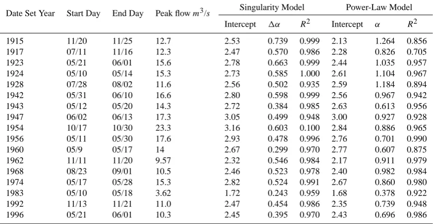
Table 3. Results obtained by means of singularity model and power-law model.
Date Set Year Start Day End Day Peak flowm3/s Singularity Model Power-Law Model
Intercept 1α R2 Intercept α R2
1915 11/20 11/25 12.7 2.53 0.739 0.999 2.13 1.264 0.856
1917 07/11 11/16 12.3 2.47 0.570 0.986 2.28 0.826 0.705
1923 05/21 06/01 15.6 2.78 0.663 0.999 2.44 1.035 0.957
1924 05/10 05/14 15.3 2.73 0.585 1.000 2.61 1.104 0.967
1928 07/28 08/02 11.6 2.56 0.502 0.935 2.59 1.184 0.894
1942 05/31 06/10 16.6 2.80 0.598 0.999 2.56 0.967 0.942
1943 05/12 05/20 14.3 2.72 0.384 0.985 2.63 0.613 0.956
1947 06/02 06/13 17.3 3.05 0.499 0.948 3.00 0.927 0.928
1954 10/17 10/30 23.3 3.16 0.603 0.100 2.84 0.886 0.965
1956 05/11 05/30 17.6 2.93 0.478 0.996 2.76 0.701 0.990
1960 05/9 05/17 14 2.67 0.299 0.970 2.77 0.607 0.875
1962 11/11 11/20 9.57 2.32 0.546 0.984 2.17 0.911 0.979
1968 08/23 09/01 10.5 2.46 0.523 0.978 2.40 0.982 0.984
1974 05/17 05/28 15.3 2.82 0.524 0.991 2.67 0.860 0.980
1983 05/10 05/18 3.62 1.72 0.243 0.959 1.68 0.378 0.922
1992 11/13 11/21 11.0 2.47 0.454 0.986 2.35 0.739 0.948
1996 05/21 06/01 10.3 2.45 0.395 0.970 2.43 0.696 0.986
following properties (Cheng and Agterberg, 1996; Cheng, 1999):
1. If1α=0 if and only ifQ∗(≤k)→constant which is in-dependent of vicinity size ofk.
2. If1α>0 if and only ifQ∗(≤k)→∞which is an in-creasing function ofkand the value tends to infinity. 3. If1α<0 if and only ifQ∗(≤k)→0 which is a
decreas-ing function ofkand the value tends to zero.
The above properties show that the index1αcan be used to quantify the order of singularity. From a numerical data processing point of view, the singularity index can be used as a high-pass filter when applied to a time series (Cheng, 1999) for identification of anomalies from normal background val-ues (Cheng, 2005, 2007a, b) and for downscaling mapping purposes (Cheng, 2008a).
If assume the power-law relation in Eq. (4) we can reorga-nize the form so that
Qk=cka−c(k−1)a=cka[1−(1− 1
k)
a]≈caka−1=cak−1a(5) It shows that the flowQitself may also be approximated by power-law relation with timekand the approximation is usu-ally good for largek. Considering peak flow usually exists for a short period of time, the approximation Eq. (5) may not be generally acceptable. Data analysis in the following sections will confirm this.
Relations in Eqs. (4) and (5) were applied to the 17 main peak flow data from the Cataract Station on Credit River in
1
Figure 4. Plots showing relations between peak flow data and time duration for testing power-law
relations (4) (top row) and (5) (middle row) and exponential relation (bottom row). Straight lines were
fitted by least squares method; log-transformation is e-based.
Fig. 4. Plots showing relations between peak flow data and time duration for testing power-law relations Eqs. (4) (top row) and (5) (middle row) and exponential relation (bottom row). Straight lines were fitted by least squares method.
values of singularity index (1α)calculated from the 17 peak flow series range from 0.20 to 0.75. These positive values indicate that the peak flow series indeed show strong singu-larity around the flow peak implying that the water volume released during the short period time around the peak flow is non-linearly proportional to the time duration. When the time becomes zero, the flow rate tends to become infinitely large. Around the singularity it is usually impossible to mea-sure actual flow value accurately and the average values de-rived from a few measurements often are not enough for ac-curate estimation of the singular flow values. However, from
Q. Cheng et al.: Characterization of peak flow events with local singularity method 511
O
b
se
r
v
e
d
a
n
d e
st
im
a
te
d pe
a
k
f
lo
w
y = -0.0032x + 6.6757 R2 = 0.41
Figure 5. Sequences of 17 flood events recorded at the Cataract station.
(A) The observed peak flow shown as dots and the estimated peak flow
as solid line; (B) The general trend of singularity ∆α values fitted with
a straight line by least square method.
(B) (A)
1
O
b
se
r
v
e
d
a
n
d e
st
im
a
te
d pe
a
k
f
y = -0.0032x + 6.6757 R2 = 0.41
Figure 5. Sequences of 17 flood events recorded at the Cataract station.
(A) The observed peak flow shown as dots and the estimated peak flow
as solid line; (B) The general trend of singularity ∆α values fitted with
a straight line by least square method.
(B)
1
Fig. 5. Sequences of 17 flood events recorded at the Cataract station. (A) The observed peak flow shown as dots and the estimated peak flow as solid line; (B) The general trend of singularity1αvalues fitted with a straight line by least square method.
peak flow and observed peak flow generally fit well. From the plot (5B) one can see that the singularity shows general decreasing trend for the time period studied with a squared correlation coefficientR2=0.41 or student t-value=3.2, indi-cating a statistically significant correlation. Similar trends are found at other stations located in other rivers, although the statistical significances vary from river to river. In order to inspect the spatial distribution of singularity of peak flow events we applied the method to all other major peak flow events recorded at other stations in all rivers studied. All cases confirm good fits of power-law relation Eq. (4) to the data of peak flowQ∗andkand the fitness obtained using the relation Eq. (4) is consistently better than that by power-law relation Eq. (5). In addition we plot the distribution of singu-larity values (1α)cross all drainage basins in the study area. Figure 6 shows one example of singularity values calculated from flood events in May 1974 in all stations.
6 Discussion and conclusions
The results described in this paper suggest the proposition that extreme hydrological flow series present the singularity property as that the amount of water released during a short period of time, and is anomalously large in comparison with normal flow series. For hydrological engineering purposes these types of extreme events are characterized by long re-turn periods. From a self-similarity of frequency and size distribution point of view, extreme events, especially those of large flooding related flow data may follow a distribu-tion type different from that of normal flow events. The use of C-A method as introduced in this paper may provide a way to separate these types of distributions. Applying this method for the historical flow data from the ORM area, we have demonstrated that, in general, the normal flow data may show power-law relationship between flow magnitude and
Figure 6. Distribution of singularity ∆α obtained from flood events occurred in May
1974 in the ORM area. Outlines of colored patterns are boundaries of drainage
basins.
Fig. 6. Distribution of singularity1αobtained from flood events
occurred in May 1974 in the ORM area. Outlines of colored pat-terns are boundaries of drainage basins.
non-linear processes, energy release and mass accumulation may follow power-law distribution with the relevant time or space involved. In addition, the singular events may describe power-law frequency distribution although usually more data or long flow data series are needed for validation. From the data used in this paper it has been demonstrated that local singularity does exist around peak flow as recorded at gaug-ing stations in the study area. The flow itself as well as time after flow peak also may follow power-law distribution (or fractal distribution). This type of fractal model already had been utilized for describing peak flow recession patterns in literature. This paper also elaborates on comparison of the ordinary power-law model with the singularity model from which it was concluded that the singularity model is gener-ally superior to the power-law flow model. As flow models form the basis for river flow prediction in both gauged and ungauged basins the new model which is based on singularity theory may provide an option for modeling flow prediction. This proposition will be further investigated.
From the data analysis using the three methods of return period, C-A plot and local singularity index, we may con-clude that in the ORM area flow events with 10 year or above return period show distinct self-similarity from the majority of flow events with small return period and strong local sin-gularity for the major flooding events.
Acknowledgements. Thanks are due to F. P. Agterberg and other
reviewers for critical reading of the paper and constructive comments. The research was financially supported by Chinese projects: Distinguished Young Researcher Grant (40525009), Strategic Research Grant (40638041), High-Tech Research and Development Grant (2006AA06Z115) and a Research Team Development Project (IRT0755).
Edited by: J. de Lima
Reviewed by: F. Agterberg and two other anonymous Referees
References
Agterberg, F. P.: Multifractal modeling of the sizes and grades of giant and supergiant deposits, Int. Geol. Rev., 37, 1–8, 1995. Bak, P., Tang, C., and Wiessenfeld, K.: Self-organized criticality:
An explanation of 1/f noise, Phys. Rev. Lett., 59, 381–384, 1987. Brutsaert, W. and Nieber, J. L.: Regionalized drought flow hydro-graphs from a mature glaciated plateau, Water Resour. Res., 13, 737–643, 1977.
Brown, D. M., Mckay, G. A., and Chapman, L. J.: The climate of southern Ontario: Climato-logical Studies, No. 5, Department of Transport, Meteorological Branch. Toronto, p. 50, 1968. Cheng, Q.: A combined power-law and exponential model for
streamflow recessions, J. Hydrol., 352, 157–167, 2008. Cheng, Q.: Modeling local scaling properties for multi-scale
map-ping, accepted by Vadose Zone Journal, 7, 525–532, 2008. Cheng, Q.: Mapping singularities with stream sediment
geochemi-cal data for prediction of undiscovered mineral deposits in Gejiu, Yunnan Prov., China, Ore Geol. Rev., 32(1–2), 314–324, 2007a.
Cheng, Qiuming: Multifractal imaging filtering and decomposition methods in space, Fourier frequency, and eigen domains, Nonlin. Processes Geophys., 14, 293–303, 2007b,
http://www.nonlin-processes-geophys.net/14/293/2007/. Cheng, Q.: Multifractal modeling of Eigenvalues and Eigenvectors
of 2-D maps, Math. Geol., 37(8), 915–927, 2005.
Cheng, Q.: Weights of evidence modeling of flowing wells in the Greater Toronto Area, Canada, Nat. Resour. Res., 13, 77–86, 2004.
Cheng, Q.: Multifractality and spatial statistics, Computers Geosci., 25(9), 949–961, 1999.
Cheng, Q. and Agterberg F. P.: Singularity analysis of ore-mineral and toxic trace elements in stream sediments, Computers Geosci., 35, 234–244, 2009.
Cheng, Q. and Agterberg, F. P.: Multifractal modeling and spatial statistics, Math. Geol., 28, 1–16, 1996.
Cheng, Q., Agterberg, F. P., and Ballantyne, S. B.: The separation of geochemical anomalies from background by fractal methods, J. Exploration Geochem., 51, 109–130, 1994.
Cheng, Q., Zhang, G., Lu, C., and Ko, C.: GIS spatial-temporal modeling of water systems in the Greater Toronto Area, Canada, Earth Sciences, a Journal of China University of Geosciences, 15, 275–282, 2004.
Cheng, Q., Ko, C., Yuan, Y., Ge, Y., and Zhang, S.: GIS Modeling for predicting river runoff volume in ungauged drainages in the Greater Toronto Area, Canada, Computers Geosci., 32(8), 1108– 1119, 2006.
Cheng, Q., Yuan, Y., Ko, C., Li, L., and Zhang, Z.: Study of wa-ter system in the Greawa-ter Toronto Area using GIS-based spatial-temporal-frequency models, in: Environmental Geosciences, edited by: Chunmiao Zheng and Xiahong Feng, Advances in Earth Sciences, Chinese High Education Press, Beijing, 4(5), 87– 118, 2008.
Cheng, Q., Russell, H., Sharpe, D., Kenny, F., and Pin, Q.: GIS-based statistical and fractal/multifractal analysis of surface stream patterns in the Oak Ridges Moraine, Computers Geosci., 27, 513–526, 2001.
Foster, H. A.: Theoretical frequency curves and their application to engineering problems, Transactions of the American Society of Civil Engineers, 77, 564–617, 1924.
Gupta, V. K.: Emergence of statistical scaling in floods on channel networks from complex runoff dynamics, Chaos, Solitons and Fractals, 19, 357–365, 2004.
Gupta, V. K. and Waymire, E. C.: Multiscaling properties of spatial rainfall and river flow distributions, J. Geophys. Res., 95(D3), 1999–2009, 1990.
Gupta, V. K., Castro, S. L., and Over, T. M.: On scaling exponents of spatial peak flows from rainfall and river network geometry, J. Hydrol., 187, 81–104, 1996.
Hall, F. R.: Base flow recession – a review, Water Resour. Res., 4, 973–983, 1968,.
Hengeveld, H. G.: Climate change digest-projections for Canada’s future, Special edition, Ministry of Public Works and Govern-ment Services: p. 27, 2000.
Hurst, H. E.: Long-term storage capacity of reservoirs, Transact. Am. Soc. Civil Eng., 116, 770–808, 1951.
IPCC; Climate change 2001: Impacts, Adaptation and Vulnerabil-ity, Cambridge University Press: p. 1005, 2001.
Jakeman, A. J. and Hornberger, G. M.: How much complexity is warranted in a rainfall-runoff model?, Water Resour. Res., 29(8), 2637–2649, 1993.
Jakeman, A. J., Littlewood, I. G, and Whitehead, P. G.: Computa-tion of the instantaneous unit hydrograph and identifiable com-ponent flows with application to two small upland catchments, J. Hydrol., 117, 275–300, 1990.
Jakeman, A. J, Post, D. A., and Beck, M. B.: From data and the-ory to environmental model: the case of rainfall-runoff, Environ-metrics, 5, 297–314, 1994.
Kenny, F. M.: A chromostereo enhanced digital elevation model of the Oak Ridges Moraine Area, southern Ontario and Lake On-tario Bathymetry, Geological Survey of Canada, Open file 3423, scale 1:200 000, 1997.
Ko, C. and Cheng, Q.: GIS spatial modeling of river flows and pre-cipitation in the ORM, Ontario, Computers Geoci., 30, 379–389, 2004.
Kundzewicz, Z, W., Rosbjerg, D., Simonovic, S. P., and Takeuchi, K.: Extreme hydrological events: Precipitation, Floods, and Droughts, IAHS No. 213, 1–7, 1993.
Maillet, E.: Essai d’hydraulique souterraine et fluviale, Libraire Sci., A., Herman, Paris (Cited by Hall, 1968), 1905.
Malamud, B. D., Turcotte, D. L., and Barton, C. C.: The 1993 Mis-sissippi river flood: a one hundred or a one thousand year event?, Environ. Eng. Geosci. II, 479–486, 1996.
Malamud, B. D., Turcotte, D. L., Guzzetti, F., and Reichenbach, P.: Landslide inventories and their statistical properties, Earth Surf. Process. Landforms, 29, 687–711, 2004.
Mitchell, W. D.: Model hydrographs, US Geol. Surv., Water Supply Pap. 2005, 1972.
Movahed, M. S. and Hermanis, E.: Fractal analysis of river flow fluctuations, Physica A, 387, 915–932, 2008.
Murdock, R. U. and Gulliver, J. S.: Prediction of river discharge at ungauged sites with analysis of uncertainty, J. Water Resour. Pl-Asce. 119, 473–487, 1993.
Nguyen, Van-Thanh-Van: On modeling of extreme hydrologic processes, in Proceedings of International Workshop on Non-structural Measures for Water Management Problems, London, Canada, October 2001, 167–180, 2001.
Sarewitz, D. and Pielke, R.x: Extreme events: A research and policy framework for disaster in context, Int. Geol. Rev., 43, 406–418, 2001.
Schertzer, D. and Lovejoy, S.: Multifractal generation of self-organized criticality, in Fractals In the natural and applied sci-ences, edited by: Novak, M. M., 325–339, Elsevier, New York, 1994.
Schertzer, D. and Lovejoy, S.: Multifractals and turbulence: Funda-mentals and Applications, 230 pp., World Scientific, River Edge, N. J., 1995.
Schertzer, D. and Lovejoy, S.: Physical modeling and analysis of rain and clouds by anisotropic scaling of multiplicative pro-cesses, J. Geophys. Res., 92, 9693–9714, 1987.
Singer, S. N., Cheng, C. K., and Scafe, M. G.: The Hydrogeology of Southern Ontario, Second Edition, Hydrogeology of Ontario Se-ries, Report 1, Environmental Monitoring and Reporting Branch, Ministry of The Environment, p. 200, 2003.
Sornette, D.: Critical Phenomena in Natural Sciences: Chaos, Frac-tals, Selforganization and Disorder, 2nd Edition. Springer, New York, 2004.
STORM-Coalition: Oak Ridges Moraine. Boston Mills Press, Erin, Ont., p. 120, 1997.
Tallaksen, L. M.: A review of baseflow recessionanalysis, J. Hy-drol., 165, 349–370, 1995.
Tessier, Y., Lovejoy, S., Hubert, P., and Schertzer, D.: Multifrac-tal analysis and modeling of rainfall and river flows and scaling, causal transfer functions, J. Geophys. Res., 101(D21), 26427– 26440, 1996.
Turcotte, D. L.: Self-organized criticality: Does it have anything to do with criticality and is it useful?, Nonlin. Processes Geophys., 8, 193–196, 2001,
http://www.nonlin-processes-geophys.net/8/193/2001/.
Turcotte, D. L.: Fractals and Chaos in Geology and Geophysics, 2nd Edition. Cambridge University Press, 1997.
Turcotte, D. L. and Greene, A.: Scale-invariant approach to flood frequency analysis, Stochastic Hydrol. Hydraul., 7, 33–40, 1993. US Department of Agriculture, Soil conservation Service: National Engineering Handbook, Section 4, Hydrology, U.S. Govt. Print-ing Office, WashPrint-ington, DC, p. 544, 1972.
Veneziano, D.: Multifractality of rainfall and scaling of intensity-duration-frequency curves, Water Resour. Res., 38, 1–12, 2002. Viessman, W. and Lewis, G. L.: Introduction to hydrology, Pearson