www.nonlin-processes-geophys.net/19/473/2012/ doi:10.5194/npg-19-473-2012
© Author(s) 2012. CC Attribution 3.0 License.
in Geophysics
Brief communication
“Improving the actual coverage of subsampling confidence intervals
in atmospheric time series analysis”
A. Gluhovsky1and T. Nielsen2
1Department of Earth, Atmospheric, and Planetary Sciences and Department of Statistics, Purdue University, West Lafayette, IN 47907, USA
2Department of Statistics, Purdue University, West Lafayette, IN 47907, USA Correspondence to: A. Gluhovsky ([email protected])
Received: 11 July 2012 – Accepted: 6 August 2012 – Published: 5 September 2012
Abstract. In atmospheric time series analysis, where only one record is typically available, subsampling (which works under the weakest assumptions among resampling methods), is especially useful. In particular, it yields large-sample con-fidence intervals of asymptotically correct coverage prob-ability. Atmospheric records, however, are often not long enough, causing a substandard coverage of subsampling con-fidence intervals. In the paper, the subsampling methodology is extended to become more applicable in such practically important cases.
1 Introduction
Observed and modeled data are often collected in the form of time series, but there are several predicaments for employ-ing traditional time series analysis in atmospheric sciences. The primary challenges are: (a) the records are frequently prohibitively short, while just a few records (typically one) are available, and (b) conventional statistical methods are “based on certain probabilistic assumptions about the nature of the physical process that generates the time series of inter-est. Such mathematical assumptions are rarely, if ever, met in practice” (Ghil et al., 2002). One common assumption is that observations are normally distributed. Yet in reality dis-tributions are often not normal, such as those for the velocity field in a turbulent flow (e.g., Lesieur, 2008), and new ad-vances in statistics have made it clear that even slight de-partures from normality can be a source of concern (e.g., Wilcox, 2003). Another questionable assumption is that of
linear models for the observed time series, such as autore-gressive moving average (ARMA) models, whereas the real data-generating mechanism (DGM) is inherently nonlinear, so that estimation commonly based on fitted linear models may be misleading (e.g., Gluhovsky and Agee, 2007).
These issues will be addressed below by considering a problem central to obtaining reliable statistical inference from limited data sets, namely, the construction of confidence intervals (CIs) for a parameter,θ, of the unknown distribution of a stationary time series from its finite record,X1, ..., Xn.
As a typical example, consider a record in Fig. 1 from Gluhovsky (2011) of the vertical velocity of wind in a con-vective boundary layer during an outbreak of a polar air mass over the Great Lakes region. The record consists of 8192 data points over about 29 km across Lake Michigan, 50 m above the lake, and it has passed a test for stationarity from Gluhovsky and Agee (1994). The sample mean, vari-ance, skewness, and kurtosis of the vertical velocity com-puted from this record are−0.04, 1.06, 0.83, and 4.10, re-spectively. The elevated skewness and kurtosis (the corre-sponding population parameters characterizing a linear time series are 0 and 3) may indicate nonlinearities in the under-lying data-generating mechanism (DGM), but these sample characteristics are just point estimates (our “best guesses”) of the true values of the parameters. Therefore, to learn how far one can trust these numbers, CIs are employed.
474 A. Gluhovsky and T. Nielsen: Improving coverage of subsampling confidence intervals 4 A. Gluhovsky and T. Nielsen: Improving coverage of subsampling confidence intervals
vide a bridge between the Lorenz model and the original gov-erning equations, whose fundamental properties they inherit, thus presenting a viable alternative to standard time series models when these are ill-suited for the atmospheric data.
Acknowledgements. This work was supported by NSF Grant AGS-1050588.
References
Ara´ujo, V., and Pacifico, M. J: Three-Dimensional Flows, Springer, 2010.
Bertail, P., Politis, D. N., and Romano, J. P.: On subsampling esti-mators with unknown rate of convergence. J. Amer. Statist. As-soc., 94, 569-579, 1999.
Collet, P. and Eckmann, J.-P.: Concepts and Results in Chaotic Dy-namics: A Short Course, Springer, 2006.
Davison, A., and Hinkley, D.: Bootstrap Methods and Their Appli-cation. Cambridge University Press, 1997.
Fan, J., and Yao, Q.: Nonlinear Time Series, Springer, 2003. Ghil, M., Allen, M. R., Dettinger, M. D., Ide, K, Kondrashov, D.,
Mann, M. E., Robertson, A. W., Saunders, A, Tian, Y., Varadi, F., and Yiou, P.: Advanced spectral methods for climate time series, Rev. Geophys., 40(1), 1–41, 2002.
Gluhovsky, A.: Energy-conserving and Hamiltonian low-order models in geophysical fluid dynamics, Nonlin. Processes Geo-phys., 13, 125–133, 2006.
Gluhovsky, A.: Statistical inference from atmospheric time series: detecting trends and coherent structures., Nonlin. Processes Geo-phys., 18, 537–544, 2011.
Gluhovsky, A. and Agee, E.: A definitive approach to turbulence statistical studies in planetary boundary layers. J. Atmos. Sci., 51, 1682–1690, 1994.
Gluhovsky, A. and Agee, E. M.: On the analysis of atmospheric and climatic time series, J. Appl. Meteorol. Climatol., 46, 1125– 1129, 2007.
Gluhovsky, A, Zihlbauer, M., and Politis, D. N.: Subsampling con-fidence intervals for parameters of atmospheric time series: block size choice and calibration, J. Stat. Comput. Simul., 75, 381–389, 2005.
Hall, P.: On symmetric bootstrap confidence intervals, J. Royal Stat. Soc. B, 50, 35–45, 1988.
Holland, M. P., Vitolo,R., Rabassa, P., Sterk, A. E., and Broer, H. W.: Extreme value laws in dynamical systems under physical observables, Physica D, 241, 497-513, 2012.
Lenschow, D., Mann, J., and Kristensen, L.: How long is long enough when measuring fluxes and other turbulence statistics? J. Atmos. Oceanic Technol., 11, 661-673, 1994.
Lesieur, M.: Turbulence in Fluids, Springer, 2008.
Lorenz, E. N.: Deterministic nonperiodic flow, J. Atmos. Sci., 20, 130-141, 1963.
Politis, D. N. and Romano, J. P.: Large sample confidence regions based on subsamples under minimal assumptions, Ann. Stat., 22, 2031-2050, 1994.
Politis, D. N., Romano, J. P., and Wolf, M.: Subsampling, Springer, 1999.
Wilcox, R. R.: Applying Contemporary Statistical Techniques, Academic Press, 2003.
0 2000 4000 6000 8000
−2
0
2
4
t, data points
V
er
tical v
elocity
, m/s
Fig. 1. Record of 20-Hz aircraft vertical velocity measurements over Lake Michigan. Figure from Gluhovsky (2011).
0 200 400 600
0.75 0.80 0.85 0.90 b Co v er age
Fig. 2. Actual coverage probabilities of 90% subsampling CIs with β= 0.50(black)) andβ= 0.42(red)) for the skewness of nonlinear time series (4) ata= 0.145andn= 2048. Horizontal green lines denote 0.85 and 0.89 levels.
Table 1. Parameters of the model time seriesXt(Eq. (4))
distribu-tion vs sample characteristics of the observed seriesWtin Fig.1.
Xt Xtata= 0.145 Wt
Mean M= 0 0 −0.04
Variance V = 1 + 2a2 ≈1.04 1.06 Skewness S=6a+8a
3
V3/2 ≈0.84 0.83
Kurtosis K=3+60a 2
+60a4
V2 ≈3.95 4.10
Fig. 1. Record of 20-Hz aircraft vertical velocity measurements over
Lake Michigan. Figure from Gluhovsky (2011).
coverage probability. Also referred to as the nominal or tar-get coverage probability (e.g., Davison and Hinkley, 1997), it is attained only if the assumptions underlying the method for the CI construction are met. Since for atmospheric time series this is rarely the case, the actual coverage probability may differ from the target level (sometimes considerably). For example, when the DGM is linear, CIs for the mean or the variance of the time series may be found analytically, but the common practice of computing CIs from fitted lin-ear models may result in erroneous CIs when the real DGM is, in fact, nonlinear (Gluhovsky and Agee, 2007). Moreover, CIs for the skewness cannot be based on linear models that imply zero skewness. Unlike standard methods of time se-ries analysis, resampling techniques provide asymptotically valid statistical inference from a single record without mak-ing questionable/unverifyable assumptions about the DGM. Among these methods, subsampling (Politis and Romano, 1994; Politis et al., 1999) works under the weakest assump-tions, which makes it particularly applicable for atmospheric data.
When the DGM (the model) is known, CIs can be con-structed using Monte Carlo (MC) simulations: one generates many records, X1, ..., Xn, from the model, computes from each record a point estimate,θˆ, of parameterθ (skewness, for example), and an estimate,Qˆ0.90, of the 0.90 quantile of the distribution of|θ− ˆθ|(i.e., about 90 % of|θ− ˆθ|values are belowQˆ0.90, and about 10 % are above). Then a symmetric 90 % CI forθis simply
(θˆ− ˆQ
0.90,θˆ+ ˆQ0.90). (1) Such exercise motivates the construction of subsampling CIs below. Similarly, by estimatingq0.05andq0.95, the 0.05 and 0.95 quantiles of the distribution of θˆ−θ, one obtains an equal-tailed 90 % CI forθas(θˆ− ˆq0.95,θˆ− ˆq0.05).
In real-life situations with unknown DGM and a single record available,X1, ..., Xn, subsampling comes to the res-cue by replacing independent, computer-generated MC re-alizations by subsamples, or blocks of consecutive observa-tions from the record,
X1, ..., Xb | {z }
b
, ..., Xi, ..., Xi+b−1
| {z }
b
, ..., Xn−b+1, ..., Xn
| {z }
b
, (2)
which retain the dependence structure of the time series (Politis et al., 1999). Underscored above are the first, inter-mediate, and the last block, all of the same lengthb(the block size) in the record containingnobservations and, therefore, n−b+1 blocks. Using quantiles estimated from subsamples in place of independent MC records, the subsampling method yields large-sample CIs of asymptotically correct coverage, when
b→ ∞ and b/n→0 as n→ ∞, (3)
assuming the existence of a nondegenerate asymptotic distri-bution forτn(Tn−θ )at some known rate τn (Politis et al., 1999). Typically,τn=nβ, β∈(0,1], andβ=0.5 when es-timatorTnis the sample mean, sample variance, etc.
Very often, however, real records (like that in Fig. 1) are not long enough to satisfy asymptotic conditions (3), which causes two problems for practical applications. First, the ac-tual coverage probability of subsampling CIs greatly depends on the choice of block sizeb, being unacceptable beyond a relatively narrow range of b values, and second, the actual coverage may differ from the target even within this range. The first problem has been handled by another resampling technique developed (Gluhovsky et al., 2005) for the opti-mal choice ofb based on the same single available record, so that one first determines the optimal block size using this technique, then runs subsampling with the optimalbto con-struct the CI. To deal with the second problem, the so-called calibration was suggested (Politis et al., 1999) and used ever since: a CI with a desired confidence level is obtained by running subsampling for the CI with the higher level. The latter may be determined via MC simulations with an ap-proximating model for the time series at hand. For example, calibration was used in Gluhovsky (2011) to achieve the de-sired 0.90 target level for the subsampling CI for the skew-ness constructed from the record in Fig. 1.
A. Gluhovsky and T. Nielsen: Improving coverage of subsampling confidence intervals 475
Table 1. Parameters of the model time seriesXt(Eq. 4) distribution vs. sample characteristics of the observed seriesWtin Fig. 1.
Xt Xtata=0.145 Wt
Mean M=0 0 −0.04
Variance V =1+2a2 ≈1.04 1.06 Skewness S=6a+8a3
V3/2 ≈0.84 0.83 Kurtosis K=3+60a2+60a4
V2 ≈3.95 4.10
2 The approximating model
When records are long enough, subsampling does not require that any model, linear or nonlinear, be fitted to the data, and it works in complex dependent data situations under the weak-est assumptions among other computer-intensive techniques. The role of an approximating model that shares statistical properties with the time series under study is twofold. It be-comes necessary for the assessment of the actual coverage of subsampling CIs via MC simulations, thus offering the opportunity denied in practice by the single observed record. From the model, one can generate numerous records, com-pute from each one the subsampling CI, and estimate its cov-erage probability by counting the fraction of times the known parameter value,θ, was within the CI. The other important role for an approximating model is to assist with the selec-tion of the confidence level in calibraselec-tion or instead with the selection of the empirical rate of convergence in the tech-nique suggested in this paper.
Consider the following model (Lenschow et al., 1994),
Xt=Yt+a(Yt2−1), (4)
whereYt is a first-order autoregressive process (AR(1)),
Yt=φYt−1+t, (5)
0< φ <1 anda are constants, andt is a white-noise pro-cess (a sequence of uncorrelated random variables with mean 0 and varianceσ2). AR(1) with a Gaussian white noise is widely employed in studies of climate as a default model for correlated time series. When the white noise in model (5) is not Gaussian, the model may exhibit nonlinear behavior and is referred to as an implicit nonlinear model (Fan and Yao, 2003), as opposed to an explicit nonlinear model (4), where AR(1) is altered with a nonlinear component.
In simulations, σ2=1−φ2 so that σY2=1, the records contain 2048 data points, andφ=0.67, which permits to im-itate the dependence structure of the vertical velocity time series in Fig. 1 as characterized by autocorrelation functions. Ata=0.145, the mean, variance, skewness, and kurtosis of Xt (in model 4) are close to the corresponding sample char-acteristics of the series (see Table 1). Thus, model (4) might provide a better description for that series than linear models, which inherently have zero skewness.
vide a bridge between the Lorenz model and the original
gov-erning equations, whose fundamental properties they inherit,
thus presenting a viable alternative to standard time series
models when these are ill-suited for the atmospheric data.
Acknowledgements. This work was supported by NSF Grant AGS-1050588.
References
Ara´ujo, V., and Pacifico, M. J: Three-Dimensional Flows, Springer, 2010.
Bertail, P., Politis, D. N., and Romano, J. P.: On subsampling esti-mators with unknown rate of convergence. J. Amer. Statist. As-soc., 94, 569-579, 1999.
Collet, P. and Eckmann, J.-P.: Concepts and Results in Chaotic Dy-namics: A Short Course, Springer, 2006.
Davison, A., and Hinkley, D.: Bootstrap Methods and Their Appli-cation. Cambridge University Press, 1997.
Fan, J., and Yao, Q.: Nonlinear Time Series, Springer, 2003. Ghil, M., Allen, M. R., Dettinger, M. D., Ide, K, Kondrashov, D.,
Mann, M. E., Robertson, A. W., Saunders, A, Tian, Y., Varadi, F., and Yiou, P.: Advanced spectral methods for climate time series, Rev. Geophys., 40(1), 1–41, 2002.
Gluhovsky, A.: Energy-conserving and Hamiltonian low-order models in geophysical fluid dynamics, Nonlin. Processes Geo-phys., 13, 125–133, 2006.
Gluhovsky, A.: Statistical inference from atmospheric time series: detecting trends and coherent structures., Nonlin. Processes Geo-phys., 18, 537–544, 2011.
Gluhovsky, A. and Agee, E.: A definitive approach to turbulence statistical studies in planetary boundary layers. J. Atmos. Sci., 51, 1682–1690, 1994.
Gluhovsky, A. and Agee, E. M.: On the analysis of atmospheric and climatic time series, J. Appl. Meteorol. Climatol., 46, 1125– 1129, 2007.
Gluhovsky, A, Zihlbauer, M., and Politis, D. N.: Subsampling con-fidence intervals for parameters of atmospheric time series: block size choice and calibration, J. Stat. Comput. Simul., 75, 381–389, 2005.
Hall, P.: On symmetric bootstrap confidence intervals, J. Royal Stat. Soc. B, 50, 35–45, 1988.
Holland, M. P., Vitolo,R., Rabassa, P., Sterk, A. E., and Broer, H. W.: Extreme value laws in dynamical systems under physical observables, Physica D, 241, 497-513, 2012.
Lenschow, D., Mann, J., and Kristensen, L.: How long is long enough when measuring fluxes and other turbulence statistics? J. Atmos. Oceanic Technol., 11, 661-673, 1994.
Lesieur, M.: Turbulence in Fluids, Springer, 2008.
Lorenz, E. N.: Deterministic nonperiodic flow, J. Atmos. Sci., 20, 130-141, 1963.
Politis, D. N. and Romano, J. P.: Large sample confidence regions based on subsamples under minimal assumptions, Ann. Stat., 22, 2031-2050, 1994.
Politis, D. N., Romano, J. P., and Wolf, M.: Subsampling, Springer, 1999.
Wilcox, R. R.: Applying Contemporary Statistical Techniques, Academic Press, 2003.
0 2000 4000 6000 8000
−2
0
2
4
t, data points
V
er
tical v
elocity
, m/s
Fig. 1. Record of 20-Hz aircraft vertical velocity measurements over Lake Michigan. Figure from Gluhovsky (2011).
0 200 400 600
0.75 0.80 0.85 0.90 b Co v er age
Fig. 2. Actual coverage probabilities of 90% subsampling CIs with β= 0.50(black)) andβ= 0.42(red)) for the skewness of nonlinear time series (4) ata= 0.145andn= 2048. Horizontal green lines denote 0.85 and 0.89 levels.
Table 1. Parameters of the model time seriesXt(Eq. (4))
distribu-tion vs sample characteristics of the observed seriesWtin Fig.1.
Xt Xtata= 0.145 Wt
Mean M= 0 0 −0.04
Variance V = 1 + 2a2
≈1.04 1.06 Skewness S=6a+8a3
V3/2 ≈0.84 0.83
Kurtosis K=3+60a2+60a4
V2 ≈3.95 4.10
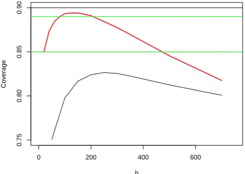
Fig. 2. Actual coverage probabilities of 90 % subsampling CIs with
β=0.50 (black) andβ=0.42 (red) for the skewness of nonlinear time series (4) ata=0.145 andn=2048. Horizontal green lines denote 0.85 and 0.89 levels.
3 Results of the simulation study
MC simulations with model (4) were carried out to explore how the actual coverage of subsampling CIs is affected by the introduction of the empirical convergence rateτn=nβ, i.e., the value of exponentβ now differs from the theoretical one (in an attempt to make for an insufficient record length and/or to avoid finding the theoretical value). Subsampling CIs for the skewness were computed according to Eq. (1), whereθˆwas the sample skewness computed from the whole
record, while the quantiles were estimated from subsamples. The latter requires decreasing the length of resulting CIs by factor of(n/b)β(Politis et al., 1999).
The black curve in Fig. 2 shows the actual coverage proba-bility of subsampling CIs for the skewness of model time se-ries (4) ata=0.145, β=0.50 for various block sizes. One can see that because of the relatively short record, the CIs are indeed useful only within a relatively narrow range of block sizes, and even then the CIs undercover (the coverage is be-low the target of 0.90). Estimating the skewness does require long records, and a simple way to improve the coverage is to increase the record length. When this is not feasible (which is typically the case), we suggest employing an “empirical” rate of convergence found via MC simulations with approxi-mating model (4). The resulting red curve demonstrates that coverage probabilities close to the target can be achieved us-ingβ=0.42 within a range of block sizes (where the curve is above, say, 0.89).
476 A. Gluhovsky and T. Nielsen: Improving coverage of subsampling confidence intervals vertical velocity skewness is positive, thus indicating
nonlin-earity in the series.
4 Conclusions
A new technique, an extension of subsampling methodol-ogy by introducing the empirical convergence rate, was sug-gested in this paper for the practically important case of short records, when subsampling CIs fail to achieve the target cov-erage probability. Its effectiveness was demonstrated for a model time series and then applied to the observed series of the vertical velocity of wind.
The construction of a subsampling CI for an unknown time series parameter requires the knowledge ofτn, the conver-gence rate of its estimator. Although the latter can also be estimated using the subsampling methodology (Bertail et al., 1999), this causes additional sampling variability in the CIs, and achieving the target coverage in case of short records still remains problematic (see Eq. 3). Finding the empirical rate, however, removes the need for the rate estimation and simultaneously improves the coverage.
As an alternative to calibration, which has been used so far to improve the coverage of subsampling CIs, the new technique has several advantages. Again, it does not require determining the rate of convergence of the estimator (still needed for calibrated CIs); it employs the same quantile estimate (say, Qˆ0.90, see Eq. 1) as the basic subsampling, whereas calibration requires higher quantiles, which are esti-mated less accurately; finally, new CIs are shorter. For exam-ple, the subsampling 90 % CI usingβ=0.42 is(0.56,1.10) for the skewness of vertical velocity time series in Fig. 1, which is smaller than the subsampling 90 % CI,(0.41,1.24), obtained in Gluhovsky (2011) via calibration withQˆ0.96. In both papers, symmetric CIs were employed. Although almost all published work on resampling CIs has focused on equal-tailed intervals, symmetric CIs are often shorter and have bet-ter coverage accuracy (Hall, 1988).
To achieve the target coverage, both calibration and the new technique require an approximating model to determine (via MC simulations) the empirical confidence level or em-pirical rate, respectively (such as model 4 for the vertical velocity time series). In general, however, the problem of selecting an approximating model is difficult, since linear models are inappropriate whereas the multitude of nonlinear models is overwhelming.
A new possibility may result from recent progress in the work that extends statistical analysis to chaotic deter-ministic dynamical systems, exemplified by the celebrated Lorenz (1963) system (e.g., Collet and Eckmann, 2006; Ara´ujo and Pacifico, 2010; Holland et al., 2012). One way to deal with formidable difficulties posed by the (determin-istic) governing equations of atmospheric dynamics is to ap-proximate them with finite systems of ordinary differential equations, the so-called low-order models (LOMs). LOMs
in the form of coupled classical mechanical systems known as the Volterra gyrostats (gyrostatic LOMs) proved partic-ularly useful, the simplest gyrostat being equivalent to the Lorenz system (Gluhovsky, 2006). Gyrostatic LOMs provide a bridge between the Lorenz model and the original gov-erning equations, whose fundamental properties they inherit, thus presenting a viable alternative to standard time series models when these are ill-suited for the atmospheric data.
Acknowledgements. This work was supported by NSF Grant
AGS-1050588.
Edited by: W. Hsieh
Reviewed by: R. V. Donner and one anonymous referee
References
Ara´ujo, V. and Pacifico, M. J: Three-Dimensional Flows, Springer, 2010.
Bertail, P., Politis, D. N., and Romano, J. P.: On subsampling esti-mators with unknown rate of convergence, J. Amer. Statist. As-soc., 94, 569–579, 1999.
Collet, P. and Eckmann, J.-P.: Concepts and Results in Chaotic Dy-namics: A Short Course, Springer, 2006.
Davison, A. and Hinkley, D.: Bootstrap Methods and Their Appli-cation, Cambridge University Press, 1997.
Fan, J. and Yao, Q.: Nonlinear Time Series, Springer, 2003. Ghil, M., Allen, M. R., Dettinger, M. D., Ide, K, Kondrashov, D.,
Mann, M. E., Robertson, A. W., Saunders, A, Tian, Y., Varadi, F., and Yiou, P.: Advanced spectral methods for climate time series, Rev. Geophys., 40, 1–41, 2002.
Gluhovsky, A.: Energy-conserving and Hamiltonian low-order models in geophysical fluid dynamics, Nonlin. Processes Geo-phys., 13, 125–133, doi:10.5194/npg-13-125-2006, 2006. Gluhovsky, A.: Statistical inference from atmospheric time series:
detecting trends and coherent structures, Nonlin. Processes Geo-phys., 18, 537–544, doi:10.5194/npg-18-537-2011, 2011. Gluhovsky, A. and Agee, E.: A definitive approach to turbulence
statistical studies in planetary boundary layers, J. Atmos. Sci., 51, 1682–1690, 1994.
Gluhovsky, A. and Agee, E. M.: On the analysis of atmospheric and climatic time series, J. Appl. Meteorol. Climatol., 46, 1125– 1129, 2007.
Gluhovsky, A., Zihlbauer, M., and Politis, D. N.: Subsampling con-fidence intervals for parameters of atmospheric time series: block size choice and calibration, J. Stat. Comput. Simul., 75, 381–389, 2005.
Hall, P.: On symmetric bootstrap confidence intervals, J. Royal Stat. Soc. B, 50, 35–45, 1988.
Holland, M. P., Vitolo, R., Rabassa, P., Sterk, A. E., and Broer, H. W.: Extreme value laws in dynamical systems under physical ob-servables, Physica D, 241, 497–513, 2012.
Lenschow, D., Mann, J., and Kristensen, L.: How long is long enough when measuring fluxes and other turbulence statistics?, J. Atmos. Oceanic Technol., 11, 661–673, 1994.
Lorenz, E. N.: Deterministic nonperiodic flow, J. Atmos. Sci., 20, 130–141, 1963.
Politis, D. N. and Romano, J. P.: Large sample confidence regions based on subsamples under minimal assumptions, Ann. Stat., 22, 2031–2050, 1994.
Politis, D. N., Romano, J. P., and Wolf, M.: Subsampling, Springer, 1999.