www.atmos-meas-tech.net/8/1875/2015/ doi:10.5194/amt-8-1875-2015
© Author(s) 2015. CC Attribution 3.0 License.
Low-level mixing height detection in coastal locations
with a scanning Doppler lidar
V. Vakkari1, E. J. O’Connor1,2, A. Nisantzi3, R. E. Mamouri3, and D. G. Hadjimitsis3 1Finnish Meteorological Institute, Helsinki, Finland
2Meteorology Department, University of Reading, Reading, UK 3Cyprus University of Technology, Limassol, Cyprus
Correspondence to: V. Vakkari ([email protected])
Received: 13 October 2014 – Published in Atmos. Meas. Tech. Discuss.: 9 December 2014 Revised: 25 March 2015 – Accepted: 27 March 2015 – Published: 23 April 2015
Abstract. Mixing layer height (MLH) is one of the key parameters in describing lower tropospheric dynamics and capturing its diurnal variability is crucial, especially for in-terpreting surface observations. In this paper we introduce a method for identifying MLH below the minimum range of a scanning Doppler lidar when operated at vertical. The method we propose is based on velocity variance in low-elevation-angle conical scanning and is applied to measure-ments in two very different coastal environmeasure-ments: Limassol, Cyprus, during summer and Loviisa, Finland, during winter. At both locations, the new method agrees well with MLH de-rived from turbulent kinetic energy dissipation rate profiles obtained from vertically pointing measurements. The low-level scanning routine frequently indicated non-zero MLH less than 100 m above the surface. Such low MLHs were more common in wintertime Loviisa on the Baltic Sea coast than during summertime in Mediterranean Limassol.
1 Introduction
Turbulent atmospheric mixing is a key process in the lower troposphere for climate, weather and air quality. Turbulent mixing is regarded as a significant player in aerosol micro-physical processes (e.g. Nilsson et al., 2001; Wehner et al., 2010; Hirsikko et al., 2013) and in cloud microphysics (e.g. Pinsky et al., 2008). Representing turbulent mixing in numer-ical models requires an understanding of the variability in space and time, the length scales involved and the processes that are responsible: friction, surface heating, shear (Bak-lanov et al., 2011). Stably stratified layers and diurnal cycles
require particular attention (Holtslag et al., 2013). From an air quality perspective, the height of the layer that is in con-stant contact with the surface, i.e. mixing layer height (MLH) is a critical parameter governing the dispersion of air pollu-tants (e.g. White et al., 2009). The continuous monitoring of the atmospheric mixing profile covering the lowest few kilo-metres is not a straightforward task and there are only a few long-term data sets (e.g. Harvey et al., 2013; Schween et al., 2014). In many studies the mixed layer is characterised indi-rectly, often in terms of MLH inferred from aerosol backscat-ter profiles (e.g. Baars et al., 2008; Korhonen et al., 2014) or temperature profiles (e.g. Beyrich and Leps, 2012). However, indirect methods in MLH estimation may potentially suffer from erroneous interpretation, especially for stably stratified layers and during the initial early morning phase or afternoon collapse of a convective boundary layer (e.g. Pearson et al., 2010; Schween et al., 2014).
the temporal resolution for routine operational launches is rather coarse; typically a maximum of four per day. Mast-based sonic anemometers provide excellent turbulent mea-surements with high temporal resolution, but masts taller than 100 m are rare; therefore remote sensing techniques are currently the only viable option for long-term continuous monitoring through the entire lower troposphere.
Several remote sensing techniques, such as Doppler sodar (e.g. Beyrich, 1997; Seibert et al., 2000; Emeis et al., 2008), Doppler lidar (e.g. Harvey et al., 2013; Schween et al., 2014) and radar wind profiler (e.g. Bianco et al., 2008; Emeis et al., 2008), enable continuous measurements of the vertical wind velocity (w) profile with high time resolution. Subse-quently, these measurements can be processed to provide ver-tical profiles of verver-tical velocity variance,σw2(e.g. Pearson et al., 2010), or turbulent kinetic energy (TKE) dissipation rate (e.g. O’Connor et al., 2010) with resolutions better than a few minutes. However, no single remote sensing instrument has been able to cover the full range of MLHs from instru-ment level up to the top of the atmospheric boundary layer. Doppler sodars can cover the low range from 10 m up to a few hundred metres, possibly reaching 1 km in good condi-tions (e.g. Emeis et al., 2008), but, in many environments, the daytime convective MLH exceeds the range of sodars. On the other hand, vertically pointing Doppler lidars and radar wind profilers are usually sensitive enough to reach the top of the atmospheric boundary layer and beyond but cannot see closer than an instrument-specific range, typically 100– 200 m (Bianco et al., 2008; Pearson et al., 2009; Srinivasulu et al., 2012), which hampers the detection of low-level only mixing.
Scanning Doppler lidars can partially overcome a min-imum height limitation by retrieving radial wind velocity measurements at a low elevation angle (Banta et al., 2006). In this paper we present a method whereby scanning Doppler lidars can identify the presence of turbulent mixing from the instrument level up, making it possible to cover the full range of potential MLHs with an appropriate selection of scan types from one instrument. From the various possible low-elevation angle scanning patterns, we selected vertical azimuth display (VAD) scans as the basis for low-level MLH detection. The main reason for choosing VAD scans is that it simultaneously provides the horizontal wind profile (e.g. Browning and Wexler, 1968) and can be utilised in study-ing the surface effects on the wind field in the vicinity of the Doppler lidar. The method for identifying turbulent mix-ing and obtainmix-ing MLH is described in Sect. 2. By apply-ing the VAD-based MLH detection to two data sets from very different environments, i.e. summertime Mediterranean coast and wintertime Baltic Sea coast, in Sect. 3, we show that this method compares well with MLH inferred from vertically pointing measurements. With this method we fre-quently identified MLHs below the lowest usable range gate of the Doppler lidar operating in vertical mode at both loca-tions.
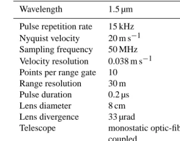
Table 1. Doppler lidar specifications.
Wavelength 1.5 µm
Pulse repetition rate 15 kHz Nyquist velocity 20 m s−1 Sampling frequency 50 MHz Velocity resolution 0.038 m s−1 Points per range gate 10
Range resolution 30 m Pulse duration 0.2 µs Lens diameter 8 cm Lens divergence 33 µrad
Telescope monostatic optic-fibre coupled
2 Methodology 2.1 Measurements
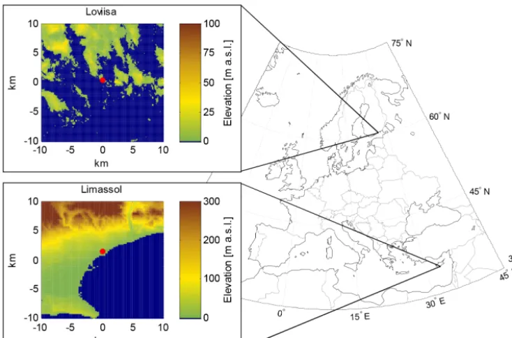
In this study we utilise Doppler lidar measurements from two locations: Limassol, Cyprus, and Loviisa, Finland (Fig. 1). Measurements were carried out with a Halo Photonics Streamline scanning Doppler lidar (Pearson et al., 2009). The Halo Photonics Streamline is a 1.5 µm pulsed Doppler lidar with a heterodyne detector that can switch between co- and cross-polar channels (Pearson et al., 2009). Standard oper-ating specifications are given in Table 1, and the minimum range of the instrument is 90 m. The accumulation time per ray varies according to scan type and location.
At Limassol, measurements were performed at the Cyprus University of Technology campus (34.6756◦N, 33.0403◦E;
15 m a.s.l.) from 22 August to 15 October 2013. Solar noon at Limassol is 09:40 UTC. The measurement site was on a rooftop 600 m NE from the Mediterranean Sea shore-line (Fig. 1). The Limassol campaign took place in typical Mediterranean summer conditions with surface temperatures ranging from+15 to+35◦C, very low cloud cover and three rain showers.
At Loviisa, the measurement campaign took place on the Fortum Power and Heat Oy nuclear power plant site on Hästholmen island (60.3660◦N, 26.3500◦E; 24 m a.s.l.) from 10 December 2013 to 17 March 2014. Solar noon at Loviisa is 10:20 UTC. Hästholmen island is approximately 2000 m long in the SE–NW direction and 500 m wide in the SW–NE direction (Fig. 1). From the measurement platform at the centre of the island, the distance to shoreline in the SW direction was 300 m and in the NE direction was 200 m. The Loviisa measurements were representative of winter condi-tions in the Baltic Sea region, characterised by surface tem-peratures ranging from −25 to +10◦C, frequent bursts of rain and snow and few cloud-free conditions.
Brown-Figure 1. Location of Loviisa and Limassol measurement sites. In the 20 km×20 km topographic map inserts for Loviisa (National Land Survey of Finland, 2014) and Limassol (United States Geological Survey, 2014) the location of the lidar is indicated by a red dot.
Table 2. Scan settings at Limassol and Loviisa. At Loviisa the 15◦
elevation angle VAD integration time was decreased from 10 to 7 s on 11 February 2014.
Site Limassol Loviisa
VAD elevation angle (◦) 10 30 4 15 Number of azimuthal angles 23 24 72 24 Integration time (s) 3 3 7 10/7 Repeat interval (min) 20 20 30 15
ing and Wexler, 1968) at 30◦ and 10◦elevation angle every 20 min (Table 2), a three-beam Doppler beam swing every 20 min as an alternative method for retrieving the vertical profile of horizontal wind (e.g. Lane et al., 2013) and a range height indicator scan every 10 min. Besides scanning, 15 out of every 20 min were available for vertically pointing mea-surements. Vertically pointing data were recorded at 3 s inte-gration time and every second beam was measured with the cross-polar receiver (Pearson et al., 2009).
At Loviisa, the terrain allowed VAD scans to be operated at a lower elevation angle than at Limassol and thus the scan schedule at Loviisa consisted of a 24-azimuthal-direction VAD scan at 15◦ elevation angle and a 72-azimuthal-direction VAD scan at 4◦elevation angle (Table 2). At Lovi-isa, vertically pointing measurements were initially operated at 8 s integration time, but on 11 February 2014 the integra-tion time was increased to 16 s. Again, every second verti-cal beam was measured with the cross-polar receiver as at
Limassol. Due to the longer integration time for each beam when scanning, there were 13 min free per 30 min for verti-cally pointing measurements. At both locations the focus of the Doppler lidar telescope was set to 2000 m. In this study we utilise only the VAD scans and co-polar vertically point-ing measurements.
Velocity measurement uncertainty is directly related to the instrument sensitivity, so there is a potential trade-off be-tween achieving the high temporal resolution suitable for in-vestigating turbulent conditions at the expense of measure-ment sensitivity and uncertainty. The integration times for each particular scan at each location were selected to achieve the highest temporal resolution possible while retaining suffi-cient sensitivity for each individual measurement; at Loviisa, a much lower atmospheric aerosol loading required a longer integration time per individual ray. Additional optimisation was required when implementing the scan schedule so that the relevant scans were acquired while still providing enough vertically pointing coverage.
2.2 Estimating turbulent mixing from a VAD
mea-0 90 180 270 360 -10
-5 0 5 10
Azimuth [ ]
VR
[m s
-1]
(a)
-2 -1 0 1 2
-2 -1 0 1 2
R [m s-1], 148 m a.s.l.
R
[m s
-1],
1
5
3
m
a
.s.
l.
R = 0.93 P = 1.2e-10 (b)
-2 -1 0 1 2
0 5 10 15 20
N
R [m s-1] (c)
148 m a.s.l. 153 m a.s.l.
03:57 2 = 0.07
11:59 2 = 0.78
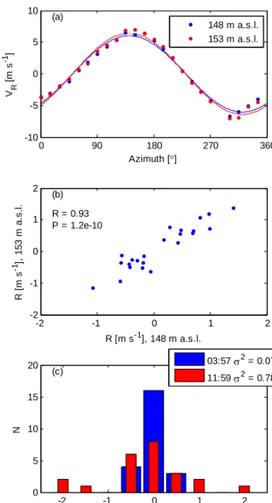
Figure 2. (a) Radial wind speed and sinusoidal fit on 24 August
2013 at 03:57 (UTC) for two consecutive altitudes from a 10◦ el-evation angle VAD scan. (b) Scatterplot of the residuals of the fit presented in panel (a). (c) Histogram of the difference of resid-uals at 148 and 153 m a.s.l. altitudes from a 10◦ elevation angle VAD scan for a calm period (03:57 UTC) and a turbulent period (11:59 UTC) with corresponding variances indicated in the legend. Theσυ2(Eq. 6) is 0.03 at 03:57 UTC and 0.04 at 11:59 UTC.
surement in a VAD, the observed radial velocity (VR)at a single range gate can be expressed analogous to the Reynolds formulation in statistical turbulence theory:
VR=Vwind+R, (1)
whereVwindis the radial component of homogeneous hori-zontal wind andRis the deviation from the homogenous hor-izontal wind. The horhor-izontal wind componentVwindis then derived by fitting a sinusoidal curve toVRas a function of the azimuthal angle (Fig. 2a) for each elevation level in a VAD, withRbeing the residuals of these fits.
Contrary to the Reynolds formulation, however, the devi-ation termR in a VAD contains more components than the purely turbulent fluctuations. These additional components
arise from fact that, over the relatively large volume of at-mosphere covered by the VAD scan, there are often non-turbulent changes in the horizontal wind speed and direction on scales of hundreds of metres to kilometres that are also contained inRin Eq. (1) whenVwindis estimated from a fit over the full VAD. In quiescent conditions, the non-turbulent contributions may even form most of the residual. This is ev-ident when correlating the residuals of two consecutive range gates as in Fig. 2b; a high correlation indicates that the resid-uals are dominated by flow patterns with length scales that are large compared to the 30 m radial resolution of the in-strument.
The contribution of some non-turbulent processes (such as translation, divergence, relative vorticity, stretching and shearing deformation) toRcan be estimated through a Taylor expansion (Browning and Wexler, 1968). However, within the first 100 m above the surface, the focus of this study,R
can also contain significant contributions from local distor-tions. Typical surface-induced changes would be wind flows around a building or wind channelling around an island. In most environments quantifying this kind of local effects with reasonable accuracy would require such detailed knowledge of the surface at the measurement location that determining turbulent contribution directly from Eq. (1) is impractical. Therefore, we consider the change inVRfrom one range gate at distancerto the next range gate at (r+30 m) for one radial measurement:
VR(r)−VR(r+30 m)=1VR=1Vwind+1R. (2) In this way, the problem of determining the non-turbulent changes in the wind field within the VAD volume has been reduced to the question of whether these changes are signifi-cant on the scale of the range resolution of the Doppler lidar. The changes in the wind field that can be represented with the Taylor expansion occur over length scales that are sig-nificantly larger than the Doppler lidar range resolution of 30 m (e.g. Browning and Wexler, 1968) and thus their contri-bution to1R can be considered negligible. Similarly, if the localised effects in the wind field can be considered smooth at the Doppler lidar range resolution scale (here 30 m), i.e. the surface is reasonably homogeneous or the measurement is not close to the surface, then we can assume also their con-tribution to1Rto be very small.
With these assumptions we can now estimate
1R≈1Vturb+υ, (3)
whereVturbis the contribution from turbulent mixing that we are interested in and
υ=pδ2(r)+δ2(r+30 m), (4)
Thus the proxy variable for identifying turbulent mixing is the variance of the difference of residuals from two consec-utive elevation levels in a VAD subtracted by the variance of the corresponding measurement uncertainty (cf. Fig. 2c):
σVAD2 (r+15 m)=1
n
n
X
i=1
1Ri− 1
n
n
X
i=1
(1Ri)
!2
(5)
−συ2,
where the subscriptirefers to individual radials andnis the number of radials within a VAD. The measurement uncer-tainty varianceσυ2is estimated from theδi2calculated for ev-eryith radial:
συ2=median(δ2(r))+median(δ2(r+30 m)), (6) where median is taken over all radials at each range gate.
The instrument uncertainty in velocity δ is primarily a function of the signal-to-noise ratio (SNR) (Pearson et al., 2009) and is calculated for every individual radial velocity measurement in a VAD. Based on pointing accuracy tests performed during both campaigns towards hard targets at known direction and distance, we consider the pointing ac-curacy error negligible especially when compared to the un-certainty arising from the measurement itself. The choice of median in Eq. (6) is to avoid outliers skewing the distribution. In general, most of the points in a particular VAD display similar sensitivity, but the presence of cloud or precipitation can increase SNR, whereas certain radials may be completely or partially obscured by buildings or trees. Measurements in the presence of precipitation have to be carefully evaluated as the signal can be dominated by the terminal fall velocity of the drop, and large drops do not necessarily track the tur-bulent motion of the air. Here, we only calculateσVAD2 when SNR > 0.0025 for at least 20 out of 24 points at any given elevation level. In terms of συ2 the SNR limit of 0.0025 is equivalent to a threshold of 1.58 m2s−2using the instrument specifications given in Table 1. This is derived by calculating
δ from SNR according to O’Connor et al. (2010) and then applying Eq. (6). Note that this assumes that the turbulence is isotropic in nature.
Abrupt changes in surface roughness also have an impact on the turbulent properties of the wind field (Garrat, 1990). For instance, the 4◦ elevation angle VAD at Loviisa is so
close to the surface that the radial wind field is clearly af-fected by the change of surface roughness moving from sea to land. To minimise the effect of surface roughness changes at Loviisa we considered only a 55◦wide sector (i.e. 12 az-imuthal directions) upwind of the island to derive MLH from the 4◦elevation angle VAD. For 10◦and higher elevation an-gle VADs we used the full 360◦to determineσVAD2 and MLH. 2.3 Turbulent kinetic energy dissipation rate
The dissipation rate of TKE was determined from the vertical velocity measurements according to the method described
by O’Connor et al. (2010). This method utilises the veloc-ity variance over a specific number of samples, from which the dissipation rate is derived using appropriate advective length scales obtained from the vertical profiles of horizontal wind. The implicit constraint in this method is that the ad-vective length scales for calculating the variance should re-main within the inertial subrange. Typically, this means that the total time available for collecting samples for one vari-ance profile should not exceed about 3 min and that the num-ber of samples available per dissipation rate profile there-fore depends on the integration time for an individual ray. For vertical profiles with 3 min resolution at Limassol, opti-mal operating conditions provided 60 vertical velocity sam-ples per dissipation rate profile. At Loviisa, a much lower at-mospheric aerosol loading required a longer integration time per individual ray to obtain sufficient sensitivity; therefore only 11 vertical velocity samples per 3 min resolution dis-sipation rate profile were available. Vertical resolution was 30 m, and dissipation rate values were determined only when the relative uncertainty in the variance was less than 1, i.e. observed variance at least twice the theoretical contribution from noise.
3 Results and discussion
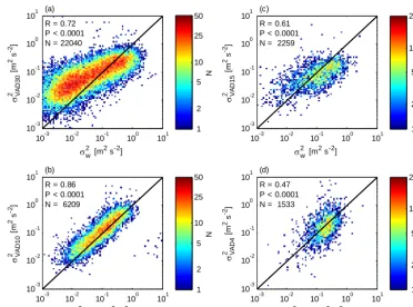
3.1 Comparison to vertical wind speed variance We first investigate how σVAD2 correlates with the vertical velocity varianceσw2 calculated directly from the vertically pointing time series. Note that we do not expectσVAD2 to be equivalent to σw2 since the effective measurement volumes can encompass very different length scales. Figure 3 shows that, at Limassol,σVAD2 from both 30 and 10◦elevation VADs correlates reasonably well withσw2. At Loviisa the correla-tion is not quite as good for the 15◦ VAD (Fig. 3), which
10-3 10-2 10-1 100 101 10-3
10-2 10-1 100 101
2 VAD15 [m
2
s-2]
2 VAD
4
[m
2 s -2]
R = 0.47 P < 0.0001 N = 1533 (d)
N
1 2 5 10 25 10-3 10-2 10-1 100 101 10-3
10-2 10-1 100 101
2 w [m
2 s-2]
2 VAD
1
5
[m
2 s -2]
R = 0.61 P < 0.0001 N = 2259 (c)
N
1 2 5 10 25
10-3 10-2 10-1 100 101 10-3
10-2 10-1 100 101
2 VAD30 [m
2
s-2]
2 VAD
1
0
[m
2 s -2]
R = 0.86 P < 0.0001 N = 6209 (b)
N
1 2 5 10 25 50 10-3 10-2 10-1 100 101 10-3
10-2 10-1 100 101
2 w [m
2 s-2]
2 VAD
3
0
[m
2 s -2]
R = 0.72 P < 0.0001 N = 22040 (a)
N
1 2 5 10 25 50
Figure 3. Frequency plots of (a)σVAD2 vs.σw2for 30◦elevation angle VAD at Limassol, (b)σVAD2 from 10◦elevation angle VAD vs.σVAD2 from 30◦elevation angle VAD at Limassol, (c)σVAD2 vs.σw2for 15◦elevation angle VAD at Loviisa and (d)σVAD2 from 4◦elevation angle VAD vs.σVAD2 from 15◦elevation angle VAD at Loviisa. Only VAD measurements for radius < 500 m are included. Theσυ2contribution (cf. Eq. 6) has been subtracted fromσw2. Correlation coefficient for logarithmic data and 1:1 line are included in all plots.
Table 3. Comparison of VAD and vertically pointing MLH estimate. For Limassol data the 25th, 50th and 75th percentile of the VAD-based
MLH are presented for the cases when the nearest-neighbour TKE-based MLH is 120 m a.s.l. For Loviisa data, the 25th, 50th and 75th percentile of the VAD-based MLH from the 15◦elevation angle VAD are presented for the cases when the nearest-neighbour TKE-based MLH is 159 m a.s.l. The 25th, 50th and 75th percentile of the VAD-based MLH from the 4◦elevation angle VAD at Loviisa are presented for the cases when the nearest-neighbour 15◦elevation angle VAD-based MLH is 55 m a.s.l.
VAD elevation VAD MLH N VAD Vertically pointing angle (◦) (m a.s.l.) percentile radius (m) MLH (m a.s.l.)
25th 50th 75th
30 105 150 195 95 182 120
10 94 145 171 119 595 120
15 170 187 230 33 504 159
4 47 50 53 26 444 55
3.2 Comparing MLH from a VAD and vertically pointing measurements
The diurnal variation of TKE dissipation rate calculated from vertically pointing measurements is plotted together with
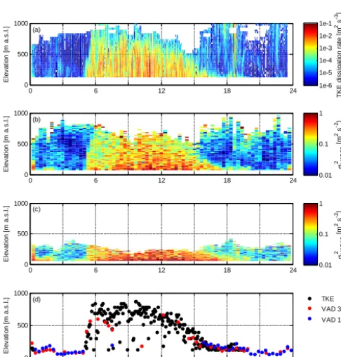
σVAD2 for Limassol in Figs. 4 and 5 and for Loviisa in Figs. 6 and 7. In a qualitative sense the diurnal dissipation rate and
σVAD2 profiles agree. The greatest difference is the instru-ment sensitivity for VADs below 15◦in elevation: the signal clearly peters out at a lower altitude than for the vertically
pointing data. This is due to two reasons: firstly, at low el-evation angles the range, or path length, to a given altitude is obviously much further than when vertically pointing and the relative rate of attenuation in the vertical plane is corre-spondingly higher; secondly, the integration time for verti-cally pointing rays can be increased without a major impact on the scan schedule.
0 6 12 18 24 0 500 1000 E le va ti o n [m a .s.l .] (a) T K E di s s ipa tion rat e [m
2 s -3] 1e-6 1e-5 1e-4 1e-3 1e-2 1e-1
0 6 12 18 24
0 500 1000 E le va ti o n [m a .s .l .] (b)
2 VA
D30
[m
2 s
-2
]
0.01 0.1 1
0 6 12 18 24
0 500 1000 E le va ti o n [m a .s. l. ] (c) 2 VAD 10 [m
2 s -2]
0.01 0.1 1
0 6 12 18 24
0 500 1000 Time UTC Ele v a tio n [m a .s
.l.] (d) TKE
VAD 30 VAD 10
Figure 4. Diurnal variation at Limassol on 24 August 2013 of (a)
TKE dissipation rate, (b)σVAD2 from 30◦elevation angle VAD, (c) σVAD2 from 10◦elevation angle VAD and (d) MLH.
0 6 12 18 24
0 500 1000 E le va ti o n [m a .s.l .] (a) T K E di s s ipa tion rat e [m
2 s -3] 1e-6 1e-5 1e-4 1e-3 1e-2 1e-1
0 6 12 18 24
0 500 1000 E le va ti o n [m a .s .l .] (b)
2 VA
D30
[m
2 s -2]
0.01 0.1 1
0 6 12 18 24
0 500 1000 E le va ti o n [m a .s. l. ] (c) 2 VAD 10 [m
2 s -2]
0.01 0.1 1
0 6 12 18 24
0 500 1000 Time UTC Ele v a tio n [m a .s
.l.] (d) TKE
VAD 30 VAD 10
Figure 5. Diurnal variation at Limassol on 17 September 2013 of (a) TKE dissipation rate, (b)σVAD2 from 30◦elevation angle VAD,
(c)σVAD2 from 10◦elevation angle VAD and (d) MLH.
0 6 12 18 24
0 250 500 E le va ti o n [m a .s.l .] (a) T K E di s s ipa tion rat e [m
2 s -3] 1e-6 1e-5 1e-4 1e-3 1e-2 1e-1
0 6 12 18 24
0 250 500 E le va ti o n [m a .s .l .] (b)
2 VA
D15
[m
2 s -2]
0.01 0.1 1
0 6 12 18 24
0 250 500 E le va ti o n [m a .s. l. ] (c) 2 VAD 4 [m
2 s -2]
0.01 0.1 1
0 6 12 18 24
0 250 500 Time UTC Ele v a tio n [m a .s
.l.] (d) TKE
VAD 15 VAD 4
Figure 6. Diurnal variation at Loviisa on 26 December 2013 of (a)
TKE dissipation rate, (b)σVAD2 from 15◦elevation angle VAD, (c) σVAD2 from 4◦elevation angle VAD and (d) MLH.
0 6 12 18 24
0 250 500 E le va ti o n [m a .s.l .] (a) T K E di s s ipa tion rat e [m
2 s -3] 1e-6 1e-5 1e-4 1e-3 1e-2 1e-1
0 6 12 18 24
0 250 500 E le va ti o n [m a .s .l .] (b)
2 VA
D15
[m
2 s -2]
0.01 0.1 1
0 6 12 18 24
0 250 500 E le va ti o n [m a .s. l. ] (c) 2 VAD 4 [m
2 s -2]
0.01 0.1 1
0 6 12 18 24
0 250 500 Time UTC Ele v a tio n [m a .s
.l.] (d) TKE
VAD 15 VAD 4
Figure 7. Diurnal variation at Loviisa on 27 December 2013 of (a)
as the altitude whereσVAD2 first drops below 0.05 m2s−2. A threshold dissipation rate of 10−4m2s−3 (cf. O’Connor et al., 2010) was selected for the vertically pointing data. In Figs. 4–7, a MLH estimate is given only if there are more data above, i.e. no MLH estimate is given if the highest data point, dissipation rate or σVAD2 , is still above the respective threshold. However, in such cases (e.g. Fig. 4c) the highest data point can be used as a lower bound for the MLH.
MLH obtained in this manner from the dissipation rate and
σVAD2 profiles are in good agreement as seen in Figs. 4–7. What is more, theσVAD2 profile can be used to check whether the mixed regions observed in the vertically pointing data are indeed connected to the surface. For instance, Limassol vertically pointing data indicate a mixed layer up to 500 m at 00:30 UTC on 24 August 2013, but σVAD2 from the 10◦ VAD shows that this turbulent region is not connected to the surface. In fact, based on the horizontal wind profile obtained from the VADs, this turbulent region lies at the lower edge of a low-level jet.
A comparison of MLH obtained from TKE dissipation rate and 30◦elevation angleσVAD2 for the full length of the cam-paign at Limassol (Fig. 8) shows a reasonable agreement between the two methods. However, as the VAD radius in-creases up to 400 m and beyond, the comparison becomes poorer. This behaviour can be expected considering that the correlation length scale of turbulence typically scales with MLH (e.g. Lothon et al., 2009). In Fig. 8 the comparison is plotted for the nearest-neighbour TKE dissipation rate for each VAD-based MLH estimate.
The connection of correlation length scale and MLH ren-ders a comparison of MLHs from vertically pointing mea-surements and lower elevation angle VADs unfeasible as the radii of 10 and 15◦ elevation angle VADs already exceed 500 m at the lowest usable range gate for vertically point-ing operation at Limassol and Loviisa (Table 3). However, when the vertically pointing measurements indicate MLH at the lowest usable range gate (i.e. a MLH of 120 m a.s.l. at Limassol and a MLH of 159 m a.s.l. at Loviisa), the 10 and 15◦elevation angle VADs also indicate a MLH in the same
range, as indicated in Table 3.
The 4◦elevation angle VAD at Loviisa is so close to the
surface that the change of surface roughness from land to sea can have a major effect on σVAD2 . To minimise the effects of local topography we have only calculatedσVAD2 from the VAD at 4◦elevation angle for a 55◦wide sector (i.e. 12 az-imuthal angles) upwind of the lidar. Then, theσVAD2 from the 4◦ elevation angle VAD agrees reasonably well withσVAD2
from the 15◦elevation angle VAD at Loviisa (Figs. 6 and 7). MLH from 4 and 15◦ elevation angle VADs also compare
well when the 15◦ elevation angle VAD indicates MLH of
55 m a.s.l. (Table 3). The width of the 55◦azimuthal sector
for the 4◦ elevation angle VAD MLH calculation is 410 m at the elevation of the lowest range gate of the 15◦elevation angle VAD.
0 100 200 300 400 500
0 100 200 300 400 500
95 104 65 30 26 17 18 12 10 N =
MLH vertical TKE [m a.s.l.]
M
L
H
V
AD
3
0
[m
a
.s
.l
.]
147 320 494 667 840
V
A
D
radius
[m
]
Figure 8. Comparison of vertical TKE dissipation-rate-based MLH
estimate andσVAD2 -based MLH for 30◦elevation angle VAD at Li-massol. Red line indicates median, blue rectangle indicates upper and lower quartiles and whiskers indicate the 10th and 90th per-centile. Black line indicates 1:1 line. The right-hand side axis indi-cates the radius of the VAD corresponding to the elevation on left-hand side axis.
3.3 Sensitivity of VAD-based MLH threshold
To check the sensitivity of the MLH determination to the choice of threshold, we varied the VAD-based MLH detec-tion threshold by±0.01 m2s−2. Increasing theσVAD2 thresh-old value decreases the MLH estimate; at Limassol, apply-ing a threshold of 0.06 m2s−2leads to, on average (mean), MLHs that are 16 m lower in the 30◦elevation angle VAD data. For the 10◦elevation angle VAD at Limassol, the higher threshold gives a 9 m lower MLH on average. Additionally, at Limassol the increasedσVAD2 threshold indicates MLH to be below the lowest usable range gate on 10 % of the cases when the 0.05 m2s−2threshold still indicates a non-zero MLH.
In the Loviisa data set, increasing the VAD-based MLH threshold has a smaller effect: for the 15◦ elevation angle
VAD the MLH estimate decreases by 11 m on average, and for the 4◦ elevation angle the MLH estimate decreases by
3 m on average. There are fewer cases at Loviisa when the increased σVAD2 threshold indicates MLH below the lowest usable range gate: 4 % of cases in the 15◦ elevation angle VAD, when the 0.05 m2s−2threshold gives a non-zero MLH; and 1 % of cases for the 4◦elevation angle VAD when the 0.05 m2s−2threshold gives a non-zero MLH.
Decreasing the σVAD2 threshold increases the MLH es-timate. At Limassol, decreasing the σVAD2 threshold from 0.05 m2s−2to 0.04 m2s−2increases the 30◦elevation angle
VAD-based MLH estimate on average by 29 m. For the 10◦ elevation angle VAD-based MLH estimate the mean increase is 17 m. At Loviisa, the respective mean increase in the 15◦ elevation angle VAD-based MLH estimate is 15 m and in the 4◦elevation angle VAD-based MLH estimate 4 m.
30 45 60 75 90 105 120 135 150 165 0
10 20 30 40 50
<30
>165
F
rac
tion [
%
]
MLH from VADs [m a.s.l.] (a)
0 3 6 9 12 15 18 21 24 0
10 20 30 40 50
(b)
F
rac
tion [
%
]
Time UTC
30 45 60 75 90 105 120 135 150 165 0
5 10 15 20 25
<30
>165 (c)
F
rac
tion [
%
]
MLH from VADs [m a.s.l.]
0 3 6 9 12 15 18 21 24 0
10 20 30 40 50
(d)
F
rac
tion [
%
]
Time UTC MLH < 30 m
MLH 30 - 150 m
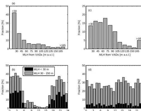
Figure 9. Histogram of MLH derived from VADs for the cases
when vertical measurements indicate MLH to be below the low-est usable range gate in vertically pointing measurement mode for Limassol (a) and Loviisa (c). The minimum range for MLH cal-culation from vertical measurements was 120 m a.s.l. at Limassol and 159 m a.s.l. at Loviisa. (b) Diurnal frequency of low MLH at Limassol. (d) Diurnal frequency of low MLH at Loviisa. The mini-mum range for MLH calculation from VADs was 30 m a.s.l. at both Limassol and Loviisa.
the changes in the VAD-based MLH due to ±0.01 m2s−2 changes in the σVAD2 threshold are small. For applications where accurate MLH detection is of critical importance, a more sophisticated MLH detection scheme than the flat threshold used here would be appropriate. The flat threshold is clearly a reasonable and robust initial estimate, and the se-lected threshold of 0.05 m2s−2gives the best agreement with the MLH inferred from the TKE profile with a threshold of 10−4m2s−3.
3.4 Frequency of low mixing level heights at Limassol and Loviisa
The vertically pointing TKE dissipation rate data close to sur-face indicate no significant mixing, implying MLH below the lowest vertical range gate at Limassol 42 % of the time and at Loviisa 62 % of the time. The VAD-based MLH estimates show that, at Limassol, in 58 % of the cases when MLH must be below the vertically pointing altitude limit, there is a shal-low mixed layer at the surface (Fig. 9). At Loviisa the VADs indicate a shallow mixed layer at the surface on 87 % of the cases when the MLH must be below the vertically pointing altitude limit (Fig. 9).
At Limassol the MLH exhibits a clear diurnal cycle with low-altitude mixing levels occurring almost exclusively dur-ing night time (Fig. 9b). This agrees with radiosonde obser-vations of mixing level heights at coastal Mediterranean lo-cations during summer (e.g. Seidel et al., 2012). At Loviisa,
however, very low MLHs are also common during daytime (Fig. 9d), typical for cold conditions with a stably stratified atmosphere and minimal surface heating (e.g. Liu and Liang, 2010).
4 Conclusions
We have shown for two very different environments that a low-elevation-angle Doppler lidar VAD scan can be used to identify the presence of turbulent mixing in the atmosphere. Although the method was developed with measurements at coastal locations, the method should be applicable in any en-vironment where VADs can be performed. Furthermore, the VAD-based proxy for turbulence can be used to identify the MLH. If scanning at a very low elevation angle is feasible at the measurement location, the VAD-based MLH can detect the presence or absence of mixing from the instrument level up. However, at elevation angles lower than 10◦, the impact of surface roughness changes across the VAD volume must be taken into consideration.
Comparison of MLHs from vertically pointing data and VADs shows reasonably good agreement, especially consid-ering the simplicity of the MLH detection scheme used here. However, the rapid increase in radius for VADs at low el-evation angles limits the altitude range of MLH retrievals from VADs. Therefore, to cover the full range of MLHs from ground level up, a combination of vertically pointing and VAD measurements are most suitable. In this manner, turbu-lent mixing can be identified from the surface up to heights of 1 km or more continuously with good time resolution. At the same time, VADs can be used to retrieve the wind profile, which in turn can be used to e.g. identify wind shear gener-ated mixing.
Finally we have demonstrated that very shallow MLHs can be present during the majority of the time when verti-cally pointing measurements indicate no mixing; i.e. MLH is below the lowest usable range gate in vertically point-ing measurement mode. At Limassol, representpoint-ing Mediter-ranean summer time conditions, such low MLHs occurred only during the night; at Loviisa, in Baltic Sea wintertime conditions, very low MLHs were also common during the day.
Acknowledgements. We gratefully acknowledge the financial
sup-port by the Nessling foundation (grants 2013006 and 201500326), the Academy of Finland Finnish Center of Excellence program (grant 1118615) as well as the support of Fennovoima Oy, Fortum Power and Heat Oy and Teollisuuden Voima Oyj under a joint research project. This work was co-funded by the European Regional Development Fund and the Republic of Cyprus through the Research Promotion Foundation (PENEK/0311/05).
References
Baars, H., Ansmann, A., Engelmann, R., and Althausen, D.: Con-tinuous monitoring of the boundary-layer top with lidar, At-mos. Chem. Phys., 8, 7281–7296, doi:10.5194/acp-8-7281-2008, 2008.
Baklanov, A. A., Grisogono, B., Bornstein, R., Mahrt, L., Zilitinke-vich, S. S., Taylor, P., Larsen, S. E., Rotach, M. W., and Fer-nando, H. J. S.: The Nature, Theory, and Modeling of Atmo-spheric Planetary Boundary Layers, Bull. Amer. Meteor. Soc., 92, 123–128, 2011.
Banta, R. M., Pichugina, Y. L., and Brewer, W. A.: Turbulent Velocity-Variance Profiles in the Stable Boundary Layer Gen-erated by a Nocturnal Low-Level Jet, J. Atmos. Sci., 63, 2700– 2719, doi:10.1175/JAS3776.1, 2006.
Beyrich, F.: Mixing height estimation from sodar data – A critical discussion, Atmos. Environ., 31, 3941–3953, doi:10.1016/S1352-2310(97)00231-8, 1997.
Beyrich, F. and Leps, J.-P.: An operational mixing height data set from routine radiosoundings at Lindenberg: Methodology, Mete-orol. Z., 21, 337–348, doi:10.1127/0941-2948/2012/0333, 2012. Bianco, L., Wilczak, J. M., and White, A. B.: Convective Bound-ary Layer Depth Estimation from Wind Profilers: Statisti-cal Comparison between an Automated Algorithm and Ex-pert Estimations, J. Atmos. Oceanic Technol., 25, 1397–1413, doi:10.1175/2008JTECHA981.1, 2008.
Browning, K. A. and Wexler, R.: The Determination of Kinematic Properties of a Wind Field Using Doppler Radar, J. Appl. Meteor., 7, 105–113, doi:10.1175/1520-0450(1968)007<0105:TDOKPO>2.0.CO;2, 1968.
Emeis, S., Schaefer, K., and Muenkel, C.: Surface-based remote sensing of the mixing-layer height – a review, Meteorol. Z., 17, 621–630, doi:10.1127/0941-2948/2008/0312, 2008.
Garrat, J. R.: The internal boundary layer – a review, Bound.-Lay. Meteorol., 50, 171–203, 1990.
Harrison, R. G. and Hogan, R. J.: In Situ Atmospheric Turbulence Measurement Using the Terrestrial Magnetic Field – A Com-pass for a Radiosonde, J. Atmos. Oceanic Technol., 23, 517–523, doi:10.1175/JTECH1860.1, 2006.
Harvey, N. J., Hogan, R. J., and Dacre, H. F.: A method to diagnose boundary-layer type using Doppler lidar, Q. J. Roy. Meteorol. Soc., 139, 1681–1693, doi:10.1002/qj.2068, 2013.
Hirsikko, A., O’Connor, E. J., Komppula, M., Korhonen, K., Pfüller, A., Giannakaki, E., Wood, C. R., Bauer-Pfundstein, M., Poikonen, A., Karppinen, T., Lonka, H., Kurri, M., Heinonen, J., Moisseev, D., Asmi, E., Aaltonen, V., Nordbo, A., Rodriguez, E., Lihavainen, H., Laaksonen, A., Lehtinen, K. E. J., Laurila, T., Petäjä, T., Kulmala, M., and Viisanen, Y.: Observing wind, aerosol particles, cloud and precipitation: Finland’s new ground-based remote-sensing network, Atmos. Meas. Tech., 7, 1351– 1375, doi:10.5194/amt-7-1351-2014, 2014.
Holtslag, A. A. M., Svensson, G., Baas, P., Basu, S., Beare, B., Bel-jaars, A. C. M., Bosveld, F. C., Cuxart, J., Lindvall, J., Steen-eveld, G. J., Tjernström, M., and Van De Wiel, B. J. H.: Stable Atmospheric Boundary Layers and Diurnal Cycles: Challenges for Weather and Climate Models, Bull. Amer. Meteor. Soc., 94, 1691–1706, doi:10.1175/BAMS-D-11-00187.1, 2013.
Khelif, D., Burns, S. P., and Friehe, C. A.: Improved wind measure-ments on research aircraft, J. Atmos. Ocean. Tech., 16, 860–875,
doi:10.1175/1520-0426(1999)016<0860:IWMORA>2.0.CO;2, 1999.
Korhonen, K., Giannakaki, E., Mielonen, T., Pfüller, A., Laakso, L., Vakkari, V., Baars, H., Engelmann, R., Beukes, J. P., Van Zyl, P. G., Ramandh, A., Ntsangwane, L., Josipovic, M., Tiitta, P., Fourie, G., Ngwana, I., Chiloane, K., and Komppula, M.: Atmo-spheric boundary layer top height in South Africa: measurements with lidar and radiosonde compared to three atmospheric models, Atmos. Chem. Phys., 14, 4263–4278, doi:10.5194/acp-14-4263-2014, 2014.
Lane, S. E., Barlow, J. F., and Wood, C. R.: An assessment of a three-beam Doppler lidar wind profiling method for use in urban areas, J. Wind Eng. Ind. Aerodyn., 119, 53–59, doi:10.1016/j.jweia.2013.05.010, 2013.
Liu, S. and Liang, X.-Z.: Observed Diurnal Cycle Climatology of Planetary Boundary Layer Height, J. Climate, 23, 5790–5809, doi:10.1175/2010JCLI3552.1, 2010.
Lothon, M., Lenschow, D., and Mayor, S.: Doppler lidar mea-surements of vertical velocity spectra in the convective plan-etary boundary layer, Bound.-Lay. Meteorol., 132, 205–226, doi:10.1007/s10546-009-9398-y, 2009.
Martin, S., Bange, J., and Beyrich, F.: Meteorological profiling of the lower troposphere using the research UAV “M2AV Carolo,” Atmos. Meas. Tech., 4, 705–716, doi:10.5194/amt-4-705-2011, 2011.
Martin, S., Beyrich, F., and Bange, J.: Observing Entrain-ment Processes Using a Small Unmanned Aerial Vehicle: A Feasibility Study, Bound.-Lay. Meteorol., 150, 449–467, doi:10.1007/s10546-013-9880-4, 2014.
Muschinski, A. and Wode, C.: First in situ evidence for coexist-ing submeter temperature and humidity sheets in the lower free troposphere, J. Atmos. Sci., 55, 2893–2906, doi:10.1175/1520-0469(1998)055<2893:FISEFC>2.0.CO;2, 1998.
National Land Survey of Finland, Elevation model 10 m, http://www.maanmittauslaitos.fi/en/NLS_open_data_licence_ version1_20120501, last access: 2 October 2014.
Nilsson, E. D., Rannik, Ü., Kulmala, M., Buzorius, G., and O’Dowd, C. D.: Effects of continental boundary layer evolution, convection, turbulence and entrainment, on aerosol formation, Tellus B, 53, 441–461, doi:10.1034/j.1600-0889.2001.530409.x, 2001.
O’Connor, E. J., Illingworth, A. J., Brooks, I. M., Westbrook, C. D., Hogan, R. J., Davies, F., and Brooks, B. J.: A Method for Estimating the Turbulent Kinetic Energy Dissipation Rate from a Vertically Pointing Doppler Lidar, and Independent Evaluation from Balloon-Borne In Situ Measurements, J. Atmos. Oceanic Technol., 27, 1652–1664, doi:10.1175/2010JTECHA1455.1, 2010.
Pearson, G., Davies, F., and Collier, C.: An Analysis of the Per-formance of the UFAM Pulsed Doppler Lidar for Observing the Boundary Layer, J. Atmos. Oceanic Technol., 26, 240–250, doi:10.1175/2008JTECHA1128.1, 2009.
Pearson, G., Davies, F., and Collier, C.: Remote sensing of the tropical rain forest boundary layer using pulsed Doppler lidar, Atmos. Chem. Phys., 10, 5891–5901, doi:10.5194/acp-10-5891-2010, 2010.
Simula-tion of Droplet Spectra EvoluSimula-tion, J. Atmos. Sci., 65, 357–374, doi:10.1175/2007JAS2358.1, 2008.
Schween, J. H., Hirsikko, A., Löhnert, U., and Crewell, S.: Mixing-layer height retrieval with ceilometer and Doppler lidar: from case studies to long-term assessment, Atmos. Meas. Tech., 7, 3685–3704, doi:10.5194/amt-7-3685-2014, 2014.
Seibert, P., Beyrich, F., Gryning, S.-E., Joffre, S., Rasmussen, A., and Tercier, P.: Review and intercomparison of operational meth-ods for the determination of the mixing height, Atmos. Environ., 34, 1001–1027, doi:10.1016/S1352-2310(99)00349-0, 2000. Seidel, D. J., Zhang, Y., Beljaars, A., Golaz, J.-C., Jacobson, A. R.,
and Medeiros, B.: Climatology of the planetary boundary layer over the continental United States and Europe, J. Geophys. Res., 117, D17106, doi:10.1029/2012JD018143, 2012.
Siebert, H., Wendisch, M., Conrath, T., Teichmann, U., and Heintzenberg, J.: A new tethered balloon-borne payload for fine-scale observations in the cloudy boundary layer, Bound.-Lay. Meteorol., 106, 461–482, doi:10.1023/A:1021242305810, 2003.
Srinivasulu, P., Yasodha, P., Kamaraj, P., Rao, T. N., Jayaraman, A., Reddy, S. N., and Satyanarayana, S.: 1280-MHz Active Array Radar Wind Profiler for Lower Atmosphere: System Description and Data Validation, J. Atmos. Oceanic Technol., 29, 1455–1470, doi:10.1175/JTECH-D-12-00030.1, 2012.
United States Geological Survey: Global Multi-resolution Terrain Elevation Data 2010, available at: http://earthexplorer.usgs.gov/, last access: 2 October 2014.
Wehner, B., Siebert, H., Ansmann, A., Ditas, F., Seifert, P., Strat-mann, F., Wiedensohler, A., Apituley, A., Shaw, R. A., Manni-nen, H. E., and Kulmala, M.: Observations of turbulence-induced new particle formation in the residual layer, Atmos. Chem. Phys., 10, 4319–4330, doi:10.5194/acp-10-4319-2010, 2010.