Nonlinear Processes
in Geophysics
c
European Geophysical Society 2001
Analytical and numerical investigation of nonlinear internal gravity
waves
S. P. Kshevetskii
Kaliningrad State University, Kaliningrad, Russia Received: 22 June 1999 – Accepted: 25 April 2000
Abstract. The propagation of long, weakly nonlinear inter-nal waves in a stratified gas is studied. Hydrodynamic equa-tions for an ideal fluid with the perfect gas law describe the atmospheric gas behaviour. If we neglect the termρ dw/dt (product of the density and vertical acceleration), we come to a so-called quasistatic model, while we name the full hydro-dynamic model as a nonquasistatic one. Both quasistatic and nonquasistatic models are used for wave simulation and the models are compared among themselves. It is shown that a smooth classical solution of a nonlinear quasistatic problem does not exist for alltbecause a gradient catastrophe of non-linear internal waves occurs. To overcome this difficulty, we search for the solution of the quasistatic problem in terms of a generalised function theory as a limit of special regularised equations containing some additional dissipation term when the dissipation factor vanishes. It is shown that such solutions of the quasistatic problem qualitatively differ from solutions of a nonquasistatic nature. It is explained by the fact that in a nonquasistatic model the vertical acceleration term plays the role of a regularizator with respect to a quasistatic model, while the solution qualitatively depends on the regularizator used. The numerical models are compared with some analyt-ical results. Within the framework of the analytanalyt-ical model, any internal wave is described as a system of wave modes; each wave mode interacts with others due to equation non-linearity. In the principal order of a perturbation theory, each wave mode is described by some equation of a KdV type. The analytical model reveals that, in a nonquasistatic model, an internal wave should disintegrate into solitons. The time of wave disintegration into solitons, the scales and amount of solitons generated are important characteristics of the non-linear process; they are found with the help of analytical and numerical investigations. Satisfactory coincidence of simu-lation outcomes with analytical ones is revealed and some examples of numerical simulations illustrating wave disinte-gration into solitons are given. The phenomenon of internal wave mixing is considered and is explained from the point of view of the results obtained. The numerical methods for in-ternal wave simulation are examined. In particular, the
influ-ence of differinflu-ence interval finiteness on a numerical solution is investigated. It is revealed that a numerical viscosity and numerical dispersion can play the role of regularizators to a nonlinear quasistatic problem. To avoid this effect, the grid steps should be taken less than some threshold values found theoretically.
1 Introduction
The majority of large-scale atmospheric and ocean models, a priori, assume a local hydrostatic equilibrium. The approx-imation corresponding to this supposition consisting of the term of a vertical acceleration is omitted is called a hydro-static or quasihydro-static approximation. Richardson has sugges-ted this simplification in 1922. One usually justifies the qua-sistatic approach by a small ratio of vertical and horizontal scales of large-scale fields;βwill denote the ratio of vertical and horizontal scales.
This justification seems quite convincing and is conven-tional now. Nevertheless, some mathematical research re-veals that the passage from a full hydrodynamic model to the limit of a quasistatic model is absent (Long, 1965; Kshevet-skii and Leble, 1985, 1988). The reason for this strange phenomenon is concealed in equation nonlinearity. Within the framework of a nonlinear hydrostatic model, at the wave front, horizontal gradients ordinarily increase with time, to-gether with vertical accelerations, which can reach infinite values over time. That is, over time, depending on initial conditions, the solution of a hydrostatic problem becomes unexistant.
The unpleasant fact would be absent if the quasistatic ap-proach was not used. It is necessary to keep only the vertical acceleration term in the equations. Actually, it is an unjusti-fied optimism. When developing a nonquasistatic model, we encounter a number of specific mathematical difficulties.
are huge in comparison with internal wave frequencies. The sound waves represent a fast mode, while the internal waves represent a slow mode. The error of any numerical method is expressed through higher derivatives of the solution. The greater these higher derivatives are, the greater the simulation error. All fast-oscillating functions have large derivatives. Therefore, high-frequency waves significantly contribute to the error and prevent numerical simulating of a slow mode.
The difficulty described cannot be overcome at the ex-pense of the diminution of difference of grid steps. On the contrary, the diminution of grid steps can only contribute to the aggravation of the outcome. Fortunately, mathematical tools are able to overcome the difficulty described. Some special numerical methods are indifferent in relation to a fast mode (Kshevetskii, 1990, 1998). These methods may be called uniformly converging methods because they meet the requirement that the convergence is uniform inβ. The uni-formly converging numerical methods are difficult ones, but they have an advantage. The errors originated from a fast mode are not accumulated over time. The methods allow one to work with the equations as if the model is a hydro-static one.
The obstacles described above do not exhaust all difficul-ties. To describe the new difficulties easier, let us return to the consideration of a quasistatic problem. As it has been mentioned, a classical smooth solution of the nonlinear qua-sistatic problem may be unexisting for larget. Such cases are not rare, but it depends on initial conditions. We take an interest in the fluid behaviour for larget. Therefore, it is nec-essary somehow to restore correctness of the problem for all t.
It is natural to try to restore the problem correctness via a conventional reception, searching for a solution in terms of generalised functions (Richtmyer, 1978). It is usual prac-tice in a nonlinear theory. Often the generalised solution is obtained as follows. At first, one adds into the equations a special term with a preceding small parameter. The newly modified equations are called regularised equations. Then one solves the regularised equations and takes the limit when the small parameter tends to zero; thus the term containing the small parameter vanishes. If, in doing so, the limit solu-tion exists, it is called a generalised solusolu-tion of the problem (Lions, 1969).
A shortcoming of the regularisation technique is that the generalised solution obtained depends on the regularisation used. In this sense, the solution is not unique. Therefore, it is very important to take the regularisation correctly. The small termρ ∂w/∂tin the nonhydrostatic model may be con-sidered as a natural regularizator. This term, in fact, fulfills the role of a regularizator because it ensures the existence of a smooth solution. However, we immediately should notice that in such conditions the effects of the numerical dissipa-tion and numerical dispersion are able to play the role of a regularizator, instead of the termρ ∂w/∂t. These numeri-cal effects always take place in all numerinumeri-cal models due to the finiteness of difference intervals. The competition be-tween different regularizators is rather probable in this case
with the effects of the numerical dissipation and numerical dispersion against the termρ ∂w/∂t. Various regularizators result in various generalised solutions. Therefore, the situa-tion requires detail study.
One can say that a nonquasistatic model is studied in the paper. However, it is more correct to consider this investi-gation differently. In this work, a usual quasistatic model is considered and various regularisation techniques are investi-gated. The nonquasistatic model is considered, but only as one of the mathematically possible regularisations. This reg-ularisation is more justified physically, and, consequently, is examined more carefully.
It is necessary to notice that the issue of equation regulari-sation is insufficiently developed for the present. As far as the author can view the question, originally it was presumed that parabolic regularisations are only physically admissible, and that the solution weakly depends on the regularisation used. Von Neumann and Richtmyer have suggested the parabolic regularisation in 1950. Later, it was discovered that the so-lution can depend on the regularisation used, but only dissi-pation terms were allowed as regularizators (Samarskiy and Popov, 1980). In the problem under consideration, a disper-sion term plays the role of a regularizator. The situation is unusual and the author could not carry out a mathematically finished investigation adequate for all practical needs of geo-physics. Nevertheless, in the paper some outcomes of sev-eral test simulations illustrating efficiency of the constructed mathematical model are shown. An effect of internal wave mixing is considered as well, as it is mathematically associ-ated with considered matters.
Dissipation effects are not taken into account. The prob-lem under consideration is two-dimensional. The simplifica-tions are not adopted because of essential difficulties. A more complete model could take dissipation and three-dimension-ality into consideration. However, within the framework of the present research, the “superfluous” terms are cut off in order to concentrate on the investigation of critical matters.
2 Basic equations and suppositions being used
The scale heightH of the atmosphere depends on heightz above the Earth’s surface. At the height of 80–90 km the ultimate velocity of internal wave propagation in the atmo-sphere reaches a minimum. Therefore, the internal waves with propagation velocities greater than√4(γ −1)gHmin/γ
can not intercross the turbopause region and therefore they propagate along the Earth’s surface horizontally. In relation to these waves, one can consider the atmosphere as a wave-guide.
into account a wave reflection effect by the turbopause re-gion. The lower boundary condition is natural.
We suppose that the atmospheric gas behaviour is gov-erned by 2D hydrodynamic equations for an ideal fluid with the perfect gas law:
dρ
dt +ρ∇·V =0, (1)
ρdu dt = −
∂P ∂x,
ρdw dt = −
∂P ∂z −ρg, cv
µρ dT
dt = −P ∇·V, P = ρRT
µ .
The labels are conventional; no special explanations are re-quired. The boundary conditions have been noted above.
We shall study, for the most part, long internal gravity wa-ves; β = kxlz 1 for long waves. Here k−x1 denotes a characteristic horizontal scale of the wave. The vertical scale islz=min(kz−1, H ), wherekzis a typical value of a vertical component of the wave vector. Using the dispersion relation for internal gravity waves, one can easily deduce the estimate ω√H /g ≈ kxlz = β 1. The symbolsωandgdenote the wave frequency and gravity acceleration. With the help of polarisation relations for internal waves, one can easily obtain the following estimates:
u
√
GH
∼ w
β√gH ∼ 1P
P0 ∼ 1ρ
ρ0 ∼ σ
Here the parameter of nonlinearityσ =1P /P01;1P,
1ρare the amplitudes of the pressure and density variations on account of wave propagation,P0,ρ0are the background
pressure and density of the unperturbed atmosphere. Some elementary estimates reveal that the vertical acceler-ations of fluid particles are small for internal waves. It means thatρ dw/dt ∼ρ0β2σ gis much less than(ρ−ρ0)g∼σρ0g
and we can considerρ dw/dtin the third equation of system (1) as small. In dimensionless variables, this term is of the orderO(β2). All other linear terms are of the identical order O(1). The nonlinear terms are of the ordersσ,σ2,σβ2. If we neglectρ dw/dt, we use a so-called quasistatic approx-imation. This approximation is very popular in geophysics. At present, it is a fundamental equation of the dynamic me-teorology.
The curvature of the Earth’s surface, the Earth’s rotation, and dissipation is not taken into account. Some estimates re-veal that these effects are not of value to resolve for nonlinear processes under consideration. Some notes concerning these effects will be made below.
3 Analytical model of nonlinear internal gravity waves
Equations (1) are very complex ones. At present, such chal-lenges may only be solved numerically. It is possible to solve (1) by a Galerkin method (Fletcher, 1984). In the framework
of a Galerkin method, a solution is sought after as a gen-eralised Fourier series with solution expansion on any com-plete set of basis functions. For example, a solution of equa-tions (1) for the horizontal velocity can be presented as the generalised Fourier seriesu(x, x, t )=P
n2n(x, t )Sn(z)on some complete set of functionsSn(z). Here2n(x, t )are fac-tors of the Fourier series. One can take the functionsSn(z) arbitrarily, if they only form a complete set. It is very con-venient in the problem under consideration to take anSn(z) those functions arise at solving the linearized equations (1 ) by a method of separation of variables.
To be sure, the solution of system (1) can be written in a linear approximation as P
n2n(x, t )Sn(z) as well. In a linear case, the solution can be constructed by a Fourier method of separation of variables. In doing so, the product 2n(x, t ) Sn(z) is often named an eigen-mode of the prob-lem, wherendenotes the mode number. The functionsSn(z) describe a vertical shape of the mode. The functionsSn(z) satisfy some Sturm-Liouville boundary value problem on ei-genvalues. This Sturm-Liouville problem automatically ari-ses when solving the linearized equations (1) by a method of separation of variables.
In a nonlinear case, we shall call the product 2n(x, t )Sn(z) a mode, by analogy to a linear theory. To supplement the Galerkin method with some “valid” simplifications based upon the smallness ofσ, β, then the set of equations (1) can be rewritten with the errorO(σ2+β4) as follows (Kshevetskii and Leble, 1985, 1988):
2nt +cn2nx+ σ 2
X
m,l
Flmn 2l2mx +β 2
2
γ −c2
n γ −1 c
3 n2nxxx
+γ +c 2 n γ −1c
3 n2
−n xxx
=0. (2)
Some modern derivation of equations (2) is given in Ap-pendix A.
The factorcn in (2) is the propagation velocity of mode nin a linear approximation. The waves with n > 0 prop-agate to the right and the waves withn < 0 propagate to the left,c−n = −cn. Flmn are the constants defining the ef-fectiveness of nonlinear interaction of modes. They are ex-pressed by rather bulky integrals, whose integrands contain functionsSn(z), Sl(z), Sm(z) and their derivatives. Equa-tions (2) are written down in dimensionless variables. That is,xis the dimensionless horizontal coordinate andtis time: xdimens.=(H /β)xnondimens.,tdimens.=β−1
√
H /gtnondimens.. The nonlinear terms in (2) are due to nonlinear terms in (1). The dispersion terms(β2/2)(γ −cn2)/(γ −1)c3n2nxxx and(β2/2)(γ+c2n)/(γ−1)c3n2−xxxn originate from the term ρ0∂w/∂tcontained in the third equation of system (1). They
is written via2n(x, t )by means of a differentiation opera-tion: w(x, z, t ) = P
n(∂2n(x, t )∂x)Sn(z)and2n(x, t ) = fn(x−cnt ). The functionsfnare arbitrary at this approxi-mation. Particular shapes ofSn(z)are not important for com-mon reasoning and, consequently, the functionsSn(z)are not written down here. One differentiation operation is contained inρ ∂w/∂t. In deriving (2), the third equation of system (1) has to be differentiated one time with respect tox. So, the third derivatives of2nhave arisen in (2).
Applyingσ = 0 andβ = 0, we shall come to a known outcome of a linear theory of long internal waves: each wave modenpropagates with the eigen velocitycnwithout chang-ing the form. Therefore, it is possible to say that equations (2) describe the nonlinear wave as a system of modes; each mode interacts with others.
Boundary conditions influence the functions Sn(z) and, subsequently, nonlinear constants Flmn. For any homoge-neous boundary conditions, internal wave propagation is de-scribed by equations such as (2). In this sense, the particular aspect of boundary conditions is not important when we are interested in qualitative nonlinear effects. It is known that long internal gravity waves propagate almost horizontally. So, if a long internal gravity wave has been excited not far from the Earth’s surface, this wave reaches the wave guide upper boundary only at large times: tdimens. ≈ h/(β
√
gH ). Therefore, system (2) is suitable also to model non-wave-guide propagation of internal waves, but only until waves have reached the heighth. We see that the boundary con-ditions do not influence the outcomes critically. For this rea-son, we have made only a slight consideration of the choice of boundary conditions.
If we neglect the interaction of various wave modes and if we take only one of them presuming that only one wave mode was originally excited, we shall obtain a KdV model of nonlinear internal waves. The KdV model has been sug-gested for the studying of nonlinear internal waves in the mid 1960’s, in a stationary variant of the KdV equation (Long, 1965; Benjamin, 1966). Between 1970 and 1980, this model was developed and was adjusted to explain various atmo-spheric and ocean processes. In contrast to the classical KdV model, equations (2) allows one to consider immediately a number of wave modes. Each of them interacts with the oth-ers. Although equations (2) do not contain z, the vertical wave propagation is taken into account in the model just as it takes place in Fourier or Calerkin methods. The history of development of a KdV model of internal waves is given briefly in Appendix B. Some references to primary sources are given there as well.
As system (2) is of extreme interest from a physical point of view, attempts were undertaken repeatedly to integrate (2) precisely. At present, some precise integrable cases are found for two- and three-wave systems. One can be found in (G¨urses and Karasu, 1996, 1998), with exhaustive infor-mation on exact integrable KdV systems and a number of references.
In the papers by the author and Leble (1985, 1988), some nonsingular perturbation theory was developed to solve (2),
and an approximate solution to this system was obtained. The approximate solution is:
2n(x, t )≈2n0(x, t )−σ
2
Z t
0
X
m,l m6=n6=l
Flmn 2l0 x−cn(t−t0), t02m0x x−cn(t−t0), t0dt0
−β 2
2
Z t
0
γ +c2n γ −1 c
3 n2
−n
0xxx(x−cn(t−t
0), t0) dt0. (3)
The functions2l0(x, t )are solutions of Korteweg-de Vries type equations (Lamb, 1980), such as
2n0t+cl2n0x+ σ 2F
n nn2n02
n 0x
+β 2
2
γ −c2n γ −1 c
3 n
!
2n0xxx =0. (4)
The initial conditions are posed so:2n0(x,0)=2n(x,0). On the right of (3), the addend takes into account nonlin-ear interaction of various modes. The nonlinnonlin-ear interaction of each wave mode with itself is taken into account imme-diately by2n0(x, t ). The approximate solution takes into ac-count various mode interactions and mode self-actions with inequality in rights. It takes place because each mode is in charge with respect to others; it loosens the interactions of the different modes. The interactions of various modes be-come apparent only at impacts of modes when wave carriers are intersected. At the same time, the nonlinear self-actions of modes continuously take place and are loosened by noth-ing. Therefore, they give the effects that are more essential. In Kshevetskii and Leble (1985, 1988), it was shown that the contributions of interaction of modesn, mare proportionate toσ/(cn−cm). For higher modes, the residuals|(cn−cm)| are small and the mode interactions are already necessary for taking into account in the principal order of the perturba-tion theory. The last term in the right-hand side of (3) takes into account some small dispersion effects. In principle, this term can be excluded, having made some appropriate com-pensatory amendments in2n0(x,0).
4 Analysis of the analytical solution
of these soliton waves is of interest as well. What do these solitons represent? Are they vortices, domains of increased or decreased pressure, something similar to a high-frequency sound wave, or something other? Now we put aside these questions, and we undertake the investigation of some ex-treme cases of interest.
The caseβ =0 is analytically analysable as well. More-over, this case is of special interest because it answers a so-called quasistatic approach; the quasistatic equation is used now as a fundamental equation of the atmosphere. Richard-son has offered the quasistatic approximation in 1922. In terms of primitive equations (1), this approximation means that the termρ dw/dt in the equation for a vertical momen-tum is omitted, and the third equation of system (1) turns into a quasistatic one
∂P
∂z +ρg=0.
In dimensionless variables, the small discarded termρ dw/dt is of the orderO(β2). The limitβ → 0 is also interesting because it corresponds to
tdimens.= 1 β
s
H
gtnondimens.→ ∞.
That is, studying the limit, we can see also what happens for largetdimens..
In terms of equations (2), atβ = 0 we have a system of quasilinear equations:
2nt +cn2nx+ σ 2
X
m,l
Fl,mn 2l2mx =0 (5)
With the errorO(σ2), this system is equivalent to the hy-drodynamic equations in the quasistatic approximation. It is well known that some waves governed by quasilinear equa-tions are able to break. More precisely, the solution may become ambiguous over time. Taking this note into account, the equations (5) were carefully investigated in Kshevetskii and Leble (1985, 1988) and Kshevetskii (1998). The condi-tion of wave breaking isFnnn2n(x, t=0)≥0. (This condi-tion can be obtained directly from (3), (4 ).) The primitive-ness of this condition reveals that the wave breaking cannot be an unusual event. If we assume that positive and nega-tive values of2n(x, t =0)are equiprobable, then, roughly speaking, the wave breaking must occur in one half of the events, at a large enought. The wave breaking demonstrates the fact that an unambiguous smooth solution (classical solu-tion) of the nonlinear quasistatic problem may be nonexistant since somet =tbreaking. Also, we come to a surprising
con-clusion: attdimens. → ∞, the solution of the hydrodynamic equations (1) does not tend in general to reach the state of a mechanical equilibrium.
The smooth, classical solution of the nonlinear quasistatic problem does not exist for allt. To overcome this difficulty, it is natural to try to consider the solution in terms of the theory of generalised functions (Richtmyer, 1978). For nonlinear equations, one ordinarily calculates it in the following way
(Lions, 1969). At first, one adds into the equations any small term ensuring the existence of a smooth solution for allt(5). This additional term is especially selected. The special term is called a regularizator and the revised equations are named regularised equations. When we have solved the regularised problem, we direct the factor preceding the small additional term to zero, and the term entered disappears. If, in doing so, the limit of the smooth solution of the regularised equations exists for allt, this limit is called a generalised solution of the problem. To be sure, the generalised solution obtained in such a way in general is not smooth. The shortcoming of the approach is that it is possible to get various generalised solutions for the same initial problem, by using various reg-ularizators. Therefore, a correct choice of the regularizator is of great importance. The choice is determined by not only some mathematical means, but also for physical reasons as well.
Let us analyse our problem. We know that2nxxx
→ ∞at
the point of wave breaking. Thereby, neglect of β22γ−cn2 γ−1c
3 n
2nxxx is inadmissible. The dispersion β22 γ−cn2 γ−1cn32nxxx
just prevents wave breaking, and it ensures the existence of a smooth solution. Therefore, the small dispersion terms β22 ·
c2
n γ−1c
3 n2nxxx
play the role of regularizators. The derivation of equations (2) reveals that the terms β22γ−c2n
γ−1c 3 n2nxxx
in (2) originate from ρ0∂w/∂t in (1). Hence, one must
and numerical dissipation should “concede”. It is difficult to ensure realisation of this requirement because usually the termρ dw/dt is very small, while both the numerical dis-persion and numerical dissipation are ineradicable due to the finiteness of difference grid steps.
Now we understand the problem specifically, and we are able to formulate some research purposes:
1. To construct a computational model of propagation of nonlinear internal gravity waves in a stratified gas. 2. To investigate a quasistatic limit.
3. To study experimentally the influence of various regu-larizators on the solution behaviour.
4. To validate the numerical model quality with the help of some special tests based upon the analytical model. 5. To investigate numerically the disintegration of internal
gravity waves into solitons.
6. To make use of obtained results to explain some physi-cal phenomena.
The order of these topics will differ from the sectional or-der for the sake of convenience.
5 Numerical simulation of nonlinear wave propagation
5.1 The numerical model
Penencko (1985), Peckelis (1988), Tapp and White (1976) and Klemp (1978) constructed nonquasistatic nonlinear models of atmospheric processes. In view of the complexity of the considered equations, some methods of decomposition were widely used to solve them. The models created were not specially aimed at the study of nonlinear internal waves. They were not tested with this class of solutions. Therefore, without additional investigation, it is difficult to tell which method is better for solving the problem.
Let us note some delicacies of numerical integration of gas dynamics equations which originate from the specificity of the problem under consideration.
a) We are interested in internal gravity waves, but acous-tic waves exist in a compressible fluid as well. Acous-tic waves are excited due to nonlinear effects, as well as through the approximations in numerical methods. Acoustic waves are capable of generating significant er-rors at numerical simulations, even if the wave ampli-tudes are small ones. In reality, the approximation error of any numerical method is expressed through the sim-ulation of some higher derivatives of the solution. The acoustic wave frequencies are high and, respectively, the higher derivatives are great. We amplify the pre-vious statement: we are interested in periods that are longer than the internal gravity wave quasiperiods. The periods are huge in comparison to the acoustic wave
quasiperiods. The numerical simulation errors have the possibility of accumulating for very long time. Eventu-ally, the numerical solution can essentially differ from the exact one, even if the numerical method is stable. Thereby, we can only hope for some special numeri-cal methods in which the errors associated with acoustic waves are not accumulated.
b) It follows from the analytical theory that, at greater time periods, the solution behaviour is strongly dependent on the ratio between the dispersion termρ ∂w/∂t (product of the density and vertical acceleration of fluid parti-cles) and nonlinear terms. All the terms mentioned are small for the problem under consideration. Therefore, with the intension of investigating nonlinear effects, we should make the simulation errors even smaller. c) An artificial or numerical dissipation is always used to
stabilize the numerical simulation of nonlinear gas dy-namics. A vanishing numerical dissipation is necessary in order to regularise an acoustic mode of the solution. The specificity of the problem under consideration is that the numerical dissipation can render a huge influ-ence on internal gravity waves. Let us consider a mo-del example. By adding a small artificial dissipation νBn2nxxxinto a KdV equation we convert this equation into a KdV-Burgers equation:
2nt +cn2nx+σ an2n2nx+β2bn2nxxx
+νBn2nxx =0 (6)
Among the numerical methods of the second order of ac-curacy, some numerical schemes that are more suitable are present. However, it was shown (Kshevetskii, 1995) that the time stepτ as well the steph1along a horizontal coordinate
must satisfy inequalities:
τ 4
s
H
g, h1
√
2H. (7)
Otherwise, numerical effects of dissipation or dispersion will play the role of a regularizator of the nonlinear problem in-stead of the termρ dw/dt. This will considerably change the behaviour of the nonlinear internal gravity waves and is inadmissible. We note the uncommonness of this statement. Such subtle questions were not formerly considered in the literature.
Careful numerical experiments have revealed that even computer roundings essentially influence the numerical solu-tion. The effects of computer roundings are well known, but they seldom are important in practice. Their present impor-tance can be explained by two circumsimpor-tances. First, we solve the problem for large intervals of heights (0−100 km), while the atmospheric gas density is exponentially decreasing with height. Secondly, we are interested in the behaviour of at-mospheric parameters for large time spans. The influence of rounding errors can be imperceptible during one hour. Nev-ertheless, the effect becomes significant for large time spans, because small rounding errors are accumulated over time. To avoid the rounding error effect, the calculations were organ-ised in a special way. At each integrating step, the wave com-ponents in relation to the background pressure, density, and temperature were calculated as preliminary ones and then the pressure, density and temperature were calculated by means of adding the wave components to the background values.
Due to the research, some special numerical models were constructed. In a linear quasistatic approximation, the nu-merical scheme developed is analogous to the scheme sug-gested by Yudin and Gavrilov (1985), but is slightly advan-ced. Some special grid of the type “cross” (Samarskiy and Popov, 1980) has been used in order that the difference equa-tions are more exact. In addition, the grid “cross” is con-venient because it easily allows the inspecting realisation of conservation laws.
The numerical scheme constructed is very similar to the two-step Lax-Wendroff scheme (Richtmyer and Morton, 1967). Therefore, it is convenient to describe the algorithm peculiarities by starting with this known scheme. Lax and Wendroff considered the hydrodynamic conservation laws rt+(q(r))x+(s(r))z=0.
Herer is a vector function, whose components are the den-sity, momentum density and energy density. Lax and Wen-droff have approximated these conservation laws as follows:
ri,kj+1−ri,kj
τ +
qj+
1 2
i+12,k(r)−q j+1
2
i−12,k(r) h1
+
sj+
1 2
i,k+1 2
(r)−sj+
1 2
i,k−1 2
(r)
h2
=0.
Hereτ is a time step,h1,h2are spatial steps that are
hori-zontal and vertical. A deviation from the usual gas dynamics equations considered by Lax and Wendroff, we take into con-sideration the gravity in the equation for momentum density. With the point of view of numerical methods, this deviation does not entail any serious difficulties.
More importantly, the mathematical difference of our scheme in comparison to the classical one is that an implicit approximation is used at the first half-step:
2r j+1
2
i,k −r j i,k
τ +
qj+
1 2
i+1 2,k
(r)−qj+
1 2
i−1 2,k
(r)
h1
+
sj+
1 2
i,k+12(r)−s
j+1 2
i,k−12(r)
h2
=0.
It certainly complicates the computations. However, this pe-culiarity of the scheme is very important. (The errors origi-nating from the acoustic waves are not only accumulated in the difference schemes of such a structure.)
The numerical scheme constructed has one additional dif-ference from the classical Lax-Wendroff scheme. One can use the numerical scheme to simulate processes in which si-multaneously, both internal gravity waves and acoustic waves take part. We already noted that a vanishing dissipation is necessary as a regularizator for acoustic waves. However, this numerical dissipation must not influence internal grav-ity waves. It is reasonable to enter the numerical dissipa-tion for acoustic waves by using “downstream differences” for approximating spatial derivatives ind(ρw)/dt. This ap-proximation introduces some additional effects of a vanish-ing nonlinear dissipation. However, the resultvanish-ing numerical dissipation renders minimum influence on internal gravity waves because the termd(ρw)/dtis very small for internal gravity waves. The numerical scheme as it stands contains two various selectively operating regularizators.
We note especially that no additional addends are into-duced into the equations. All useful qualities of the method are achieved in conventional receptions, but at the expense of successful selection of difference approximations and use of sufficiently small steps of the difference grid. Some small amendments improving dispersion relation and diminishing scheme sensitivity to the choice of grid steps were made as well.
Horizontal coordinate (1000 km)
H
o
ri
zo
n
ta
l v
e
lo
ci
ty
(m
/s
)
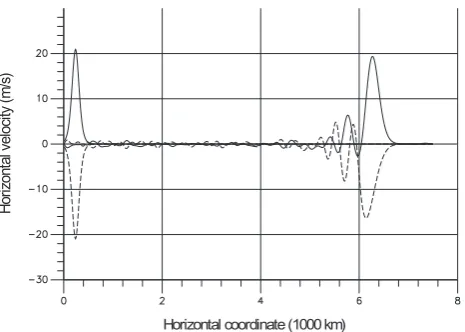
Fig. 1. Propagation of a soliton. The height is equal 98 km. Prop-agation of the wave having an opposite sign at zero time is repre-sented for comparison by a dotted line.
5.2 Comparison of analytical and numerical models We shall show here some outcomes of numerical simulation of nonlinear internal waves and we shall compare them with the analytical model. The background parameters were se-lected for the Earth’s atmosphere conditions (100 km). For simplification, the scale heightHis a constant (H =8 km), dissipation effects are not taken into account. The boundary conditions of a rigid cover are imposed at the Earth’s surface and at the height 100 km.
The analytical model shows that wave modes behave qua-si-independently, if the wave amplitude is sufficiently small. Therefore, the example of a one-mode wave is sufficient to verify analytical outcomes. At that, it reveals the essence of nonlinear processes in the best way. The first mode of inter-nal waves was selected for tests. In the ainter-nalytical model, for simplification, we have neglected the nonlinear interaction of this mode with others. Within the framework of the analyt-ical model, the considered wave propagates strictly horizon-tally. To be sure, the numerical hydrodynamic model takes into account all nonlinear effects.
In the analytical model, the hydrodynamic functions are expressed through2nas follows:
u(x, z, t )=2n(x, t )
·(A1sin(kzz)+B1cos(kzz))exp
z
2H
,
w(x, z, t )= −cn ∂ ∂x2
n(x, t )sin(k zz) exp
z
2H
,
1P (x, z, t )=gH 2n(x, t )
·(A2sin(kzz)+B2cos(kzz)) exp
− z
2H
ρ00,
1ρ(x, z, t )=2n(x, t )
·(A3sin(kzz)+B3cos(kzz))exp
− z
2H
ρ00,
A1=
cng(2−γ ) 2(c2
n−γ gH )
, A2=
c2n(γ−2) 2H (γ gH−c2
n) ,
Horizontal coordinate (1000 km)
H
o
ri
zo
n
ta
l v
e
lo
ci
ty
(m
/s
)
Fig. 2. Propagation of a soliton. The height is equal 82 km. Prop-agation of the wave having an opposite sign at zero time is shown for comparison by a dotted line.
A3=
c2n−2gH (γ −1) 2H (c2
n−γ gH )
, B1=
γ gH kzcn γ gH −c2
n ,
B2=
cn2γ kz γ gH −c2
n
, B3=
c2nkz −c2
n+γ gH ,
c2n= 4(γ −1)gH
γ (1+4kz2H2) .
Hereuandware the horizontal and vertical velocities;1P, 1ρ are the wave components to the background pressure P0(z) = ρ0(z)gH and the background density ρ0(z) =
ρ00exp(−z/H ); ρ00 is the density at the Earth’s surface;
kz = nπ/(waveguideheight)is a vertical component of the wave vector. For the first mode,n=1.
The Korteweg-de Vries equation (4) for the mode withn=
1, in dimensional variables, looks like 2nt +1.03pgH 2nx−212
r
g H2
n2n x
+0.478H2pgH 2nxxx =0. (8)
In order to allow for no errors in the test example, all calcu-lations were carried out with the help of the Derive program. If the initial condition of the Korteweg-de Vries equation (8) is as follows
2n(x,0)= −6N (N+1)0.478H 3
212L2 cosh
−2
x−x
0
L
, (9) then exactlyN solitons will be generated att → ∞(Lamb, 1980). We will use this fact for our tests.
Hotizontal coordinate (1000 km)
H
o
ri
zo
n
ta
l v
e
lo
ci
ty
(m
/s
)
Fig. 3. Propagation of a 4-soliton wave. The height is equal 66 km. For comparison, a dotted line displays propagation of the wave having an opposite sign at zero time.
with the analytical ones. Nevertheless, some parasitic small-amplitude waves are observed. Probably, one can explain it by the fact that the analytical soliton solution is only an ap-proximate one. The nonlinear effects are feeble, but the wave amplitude is also small. Unfortunately, now we know of no analytical solutions for internal waves of considerable ampli-tudes.
The disintegration of a nonlinear internal wave into soli-tons is a very bright physical process. The propagation of a disintegrating 4-soliton wave is shown in Figs. 3, 4. The initial conditions had been taken so that precisely four soli-tons were eventually generated (that is,N =4 in (9)). The initial conditions are shown on the left by a solid line and the wave after 313 minutes is represented on the right. We see that three solitons were generated at the instant shown in the figures. The outcomes of numerical experiments are in an acceptable consent with the outcomes of analytical research (Kshevetskii and Leble, 1985, 1988; Kshevetskii, 1998).
When one keeps in mind the typical atmospheric waves, then the wave amplitude may be considered as a bit exces-sive. The amplitude of the horizontal velocity is equal to 150 m/s at the height 98 km, while actually the wind at less than 150 m/s is more probable for these heights. However, in our test example we have not taken into consideration the dependence ofHonz. This dependence would lead to a par-tial wave reflection from the mesopause region and, conse-quently, the actual wave amplitude would be less. We could use the 4-soliton wave of a smaller amplitude by taking the parameterLsmaller. This parameter is a free one, and we have selected it to facilitate the numerical simulation. It is more difficult technically to carry out numerical experiments with waves of smaller amplitudes. Supposing we have used the initial conditions for the 4-soliton wave with the ampli-tude smaller byp times, then the scaleL of the 4-soliton wave would be larger by√p times. The time of disintegra-tion of such a wave would be longer byp√ptimes. It com-plicates the research because the danger of numerical error
Horizontal coordinate (1000 km)
H
ori
zo
nt
al
v
elo
ci
ty
(m
/s
)
Fig. 4. Propagation of a 4-soliton wave. The height is equal 98 km.
accumulation is increasing. At the same time, such updating of the initial conditions can provide no new outcomes. The less the wave amplitude is, the more precisely the analytical theory works. It is evident.
The wave disintegration is a corollary of nonlinearity. To demonstrate it, the propagation of the wave having an oppo-site sign in initial conditions is shown by a dashed line in Fig. 3. We see that wave disintegration does not happen in this case. It confirms the outcome obtained analytically. The steepness of this wave increases not at the wave front, but at the back. This perfectly agrees with the analytical outcomes as well.
Notwithstanding coincidence of many details, the analyti-cal formulas are somewhat rough. They display the vertianalyti-cal wave structure inaccurately. The amplitude of the numeri-cal solution grows with height faster than the amplitude of the analytical one. Probably, we would achieve better co-incidence of outcomes if we had taken into consideration, in the analytical formulas, the nonlinear effects of induced perturbation of other modes by our mode, at the expense of nonlinear effects (Kshevetskii and Leble, 1985, 1988).
It is possible to see in consideration of the analytical for-mulas that each soliton of the first wave mode is a vortex. Therefore, one can interpret the disintegration into solitons as a disintegration of an initial vortex into more small-scale vortexes.
A characteristic wave tail similar to turbulence is left be-hind the principal wave. It fails to explain this wave tail by numerical effects, because the grid steps are much less than the typical scale of oscillations in the tail. This wave turbu-lent tail is not the tail described by a non-soliton solution of a KdV equation, because the wave tail propagates too slowly. It is known that the internal waves of short vertical scales have small propagation velocities. The wave tail consists of such short waves along the vertical. The reasons for the wave tail generation are not quite understood; this effect is not yet investigated.
Horizontal coordinate (1000 km)
H
ori
zo
nt
al
v
elo
ci
ty
(m
/s
)
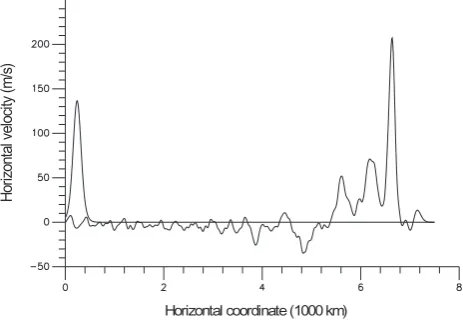
Fig. 5. Wave propagation corresponding to the same initial condi-tions as in 4-soliton case, but in a quasistatic model. The height is equal 84 km. No regularization is utilized. The wave is wrecked.
are nonsmooth or almost nonsmooth waves. The wave tail consists of small-scale vortices. It is possible to put for-ward the following hypothesis explaining the tail irregular-ity. The dispersion constantsβ22γ−c2n
γ−1c 3 n
are very small for short waves along the vertical. The wave tail consists of such waves. The constants are small of the orderO(β2/n3),nis the mode number,nis large because short waves along the vertical are considered. The less the values of the dispersion constants are, the shorter the solitons generated through dis-integration. That is, if one accepts that the tail consists of solitons of higher modes, then the solitons in the tail should be of very small horizontal scales. We concluded that short waves along the vertical have to become short along the hor-izontal, at the expense of wave disintegration. It takes place in Figs. 3, 4 actually: the generation of some nonstationary structure consisting of a number of small vortices remaining behind the head wave.
The quasistatic approach is very popular in atmospheric models because essentially it simplifies simulation. How-ever, the analytical theory reveals that the solution of a non-linear quasistatic problem can be nonexistant for somet. To verify this conclusion, some special numerical experiments were carried out. The term of vertical acceleration in hy-drodynamic equations was discarded, and then the equations were solved numerically. In Fig. 5, the behaviour of the same wave as in the 4-soliton case is shown, but within the framework of a quasistatic approach. Some time later, dur-ing “normal evolution”, the wave collapses and a simulation emergency stop arises.
Usually one achieves correctness of such nonlinear prob-lems by means of adding some vanishing artificial (or nu-merical) dissipation. Under our prognoses, such a method of problem regularisation should result in the wave like a shock wave. We cannot bypass this interesting and intrigu-ing subject. The outcome of a numerical simulation of non-linear internal waves with the quasistatic model regularised
Horizontal coordinate (1000 km)
H
o
ri
zo
n
ta
l v
e
lo
ci
ty
(m
/s
)
Fig. 6. Propagation of the wave corresponding to the same initial conditions as in 4-soliton case, but in a quasistatic model. A van-ishing artificial dissipation was used as a regularizator. A “shock wave” is formed. The height is equal 84 km.
with a vanishing artificial viscosity is shown in Fig. 6. The initial conditions are the same as in the case with four soli-tons. The vanishing dissipation has completely stabilised the wave behaviour and the wave behaves similarly to a shock wave. However, the trajectories of liquid particles are differ-ent ones. A shock wave is a wave of compression and the particles move perpendicularly to the shock wave wavefront. In the present case, we observe a propagating vortex and, at the wave front, the particles move in parallel to the wave-front. In the course of time, the vortex is strongly deformed on the front. Disintegration of this vortex into small-scale vortexes does not take place within the approach under con-sideration.
The solution obtained is independent of the artificial vis-cosity factor and one can consider it as one of several possi-ble generalised solutions of a quasistatic propossi-blem. The hy-drodynamic equations, in their initial form, are very difficult for the intuitive understanding of the nature of this gener-alised solution. Equations (5) allow one to explain perfectly “mathematical effects”. So, the generalised solution obtained is nothing else but a generalised solution of the set of equa-tions (5), which is obtained from the solution of the set of equations
2nt +cn2nx+ σ 2
X
m,l
Fl,mn 2l2mx +νX m
Kmn2mxx =0,
Knn<0, (10)
by means of passage to the limitν → 0. We can easily write down an approximate analytical solution of this set of equations. The approximate solution looks like (3), (4), but the Korteweg-de Vries equation (4) must be replaced by the Burgers equation
2n0t+cl2n0x+ σ 2F
n
nn2n02n0x+νKnn2n0xx =0.
a Burgers equation provides the wave like a shock wave at ν→0. We observe such a wave in the numerical experiment conducted.
From the mathematical point of view, the generalised so-lution obtained is faultless. However, a qualitative difference from the solution of a nonquasistatic problem is obvious. An-other regularizator (artificial viscosity instead of dispersion) has generated an other generalised solution of the nonlinear problem. If we have not particularly analysed the subtle situ-ation with equsitu-ation regularissitu-ation and if we have not under-taken some special measures to guard against the numerical effects, then we would easily obtain such a “solution” even with a nonquasistatic model. For example, the investigation has shown that an implicit scheme of the first order of accu-racy inevitably produces the same outcome, even if only the incredibly severe constraintτ 3 sec (Kshevetskii, 1995) is not satisfied.
Let us discuss briefly the applicability of obtained results to the actual atmospheric waves. In the investigated model, a temperature stratification and dissipation is not taken into ac-count. The dissipation effects are negligible in the real atmo-sphere below 100 km, but exponentially increase with height, and are very significant above 250 km (Gossard and Hook, 1978; Dikiy, 1969). The analytical model and outcomes ob-tained reveal that the modes behave quasi-independently at sufficiently small amplitudes. Using several of these quasi-independent modes, we could have even simulated vertical wave propagation, down to the upper boundary. Analogy to the Fourier method is relevant here. Therefore, it is hardly probable that the upper boundary condition or dissipation being increased with height, can considerably influence the results obtained. The investigated nonlinear effects should evince one’s force irrespectively of the boundary conditions. In particular, the nonlinear disintegration of internal waves into solitary waves of smaller scales must take place in the real atmosphere.
In the paper, nonlinear waves in an incompressible fluid were not particularly studied, but these waves correspond to the limit γ → ∞. The approximation of an incompress-ible fluid is usually utilized to describe ocean waves. There-fore, the author hopes that the results obtained can be use-ful for understanding the ocean waves as well. Furthermore, now the KdV model is actively used in oceanology for the study of internal waves and interpretation of observations. The KdV model seems to be a convenient one to describe ocean waves because ocean waves propagate within a natural wave-guide. When considering atmospheric waves, we have applied the single-mode analytical KdV model for qualita-tive understanding of atmospheric nonlinear processes. We do not lay claim to a quantitative description of atmospheric nonlinear waves with such a simple model. In consideration of ocean waves, the elementary analytical model can give quite a good quantitative consent.
6 The KdV model and internal wave mixing
In oceanology, it is known that a smooth internal gravity wave can suddenly break up, generating a spot, inside which a turbulent fluid intermixing takes place. This effect is fre-quently named “internal wave mixing”. We now consider the internal mixing from the point of view of equations (2), and we shall analyse the conditions when the effect takes place.
Formula (3) gives an approximate solution of (2). Uncou-pled KdV equations (4) lie in the basis of (3). Let us take initial conditions analogous to (9)
2n0(x,0)= −αncosh−2
x−x
0
Ln
, (11)
where
αn = −
6N (N+1)H3β2γ−c2n γ−1c3n L2
nσ Fnnn
. (12)
The formulas (11), (12) can be interpreted as follows: if ini-tial conditions look like (11), then the amountN of solitons to be generated may be derived from (12). It is clear that, for fixedαnandLn, the lesscnthe more solitons will be gener-ated. Ifcn→0, thenN → ∞. The integralsR
+∞
−∞ 2
ndxare conservative values for equation (4) . Therefore, ifN → ∞, then the soliton scales tend to zero. That is, if cn is very small, then a huge number of extremely small-scale solitons will be generated. Each soliton formed gives a vortex. There-fore, the physical phenomenon under study is the same, be-cause a smooth initial wave disintegrates into a huge number of small vortexes. The constantscnare of the orderh/(nπ ), wherenis the wave mode number andhis the wave-guide depth. Consequently, the limitcn → 0 is equivalent to the limitn→ ∞. We see that only short waves along the verti-cal, that is, such thatH / lz 1, can disintegrate into many small-scale solitons. The symbollzdesignates a typical ver-tical scale of the wave. Due to the short verver-tical wave scales, the processes happening far from wave-guide boundaries, in the body of the fluid, weakly depend on the boundary condi-tions.
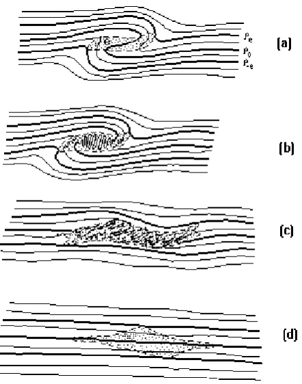
McEwan (1983) investigated experimentally the effect of “internal wave mixing”. In Fig. 7, a common picture of the considered phenomenon is shown; it is borrowed from McE-wan (1983).
According to the estimates made above, the effect takes place only for short waves along the vertical. Let us check whether this requirement is satisfied at the conditions of McEwan’s experiment (1983). In McEwan’s experiment, (gρ−1dρ/dz)1/2 ≈1.23c−1, and the tank depthlwas equal to 25 cm. Hence,H ≈ 6 m, andkz ≥ π/ l ≈4 m−1. We see thatkzH > 20 in McEwan’s experiment. Doubtlessly, McEwan dealt with short waves along the vertical.
We consider nonlinear effects for modes with largen. As noted above, the effect of the interaction of modesnandm is proportionate to(cn −cm)−1. Whenm = n+1 and at n→ ∞, the fraction denominator(cn−cn+1)is a small of
Fig. 7. Idealisation of a mixing event in a continuous stratification. (a) Overturning. (b) Development of interleaving microstructure. (c) Static stability is restored, but microstructure is preserved. (d) Gravitation to equilibrium has changed the surrounding density be-tween extremum isopycnals.
of various modes and, in order that this simplification will be correct, we have to requireαn ∼c2n/g ∼n
−2. Fortunately,
the dispersion coefficients β22 γ−c2n γ−1c
3 n
vanish very quickly atn → ∞, asc3n ∼ (√g/H (h/n))3 → 0. It rescues our idea: the amountN of solitons generated is determined only by a relationship between the nonlinearity and the dispersion, and will be huge, because the nonlinearity considerably sur-passes the dispersion. One can consider the idea as a “mathe-matical explaining” of internal wave mixing. Unfortunately, the considered model does not lead to simple and convenient working formulas. We can only suggest qualitative depen-dencies of the scalelx and quantityN of generated solitons on parameters of the disintegrating wave:
lx ∼
s
(lz)3
A , N ∼
s
AL2
l3 z
.
Herelzis a vertical scale of the broken up wave;Ais a mean amplitude of displacement of the fluid particles,Lis a hori-zontal scale of the broken up wave.
We can supplement McEwan’s outcomes with some qual-itative notes:
• IfH → ∞(or, this is the same, ifg→0), thencn→0, and the effect of wave disintegration can take place as
well. It depends on initial conditions. WhenH → ∞, the internal gravity waves turn into some stationary flow in homogeneous liquid. Hence, a fluid stratification in itself is not a reason for wave disintegration. The strati-fication only provides a bright observation of the effect.
• We try to formulate some abstract mathematical models of the phenomenon. The phenomenon exists because hydrodynamic equations have the following structure
b
N (∂ ∂t,
∂
∂x) θ (x, t )=εDθ (x, t ).b (13) HereNbis a nonlinear operator, such that a smooth
so-lution of the equationN (∂/∂t, ∂/∂x)θ (x, t )b = 0 does
not exist for somet = t1; ε 1; andεDθ (x, t )b is a
small dispersion term which plays the role of a regular-izator. The small dispersion term ensures the existence of a differentiable solution of equation (13), but this dif-ferentiable solution is quickly varying. The less ε is, the faster the solution varies. We have written spatially one-dimensional equations, but it is not important. All remaining conditions are the important ones.
• We have described above some difficulties of numerical integration of hydrodynamic equations. These difficul-ties in many respects follow from the fact that the basic equations have the structure (13). We see that the addi-tion of some small dispersion or dissipaaddi-tion terms into the equations can change the wave behaviour consider-ably. This sensitivity in relationship to terms containing higher derivatives takes place because a smooth solution of the equationN (∂/∂t, ∂/∂x)θ (x, t )b =0 does not
ex-ist for somet =t1. We deal with certain specific cases
of a nonlinear system instability.
7 Conclusions
1. Hydrostatic and nonhydrostatic numerical hydrodyna-mic models of nonlinear internal wave propagation are developed. Also, an analytical model is developed and is used to explain nonlinear wave behaviour.
2. The nonlinear disintegration of internal waves into so-litary waves of smaller scales is simulated. The com-parison of the outcomes of numerical simulation with analytical ones has shown qualitative consent. For ex-ample, the quantity of solitons generated is displayed precisely.
3. Numerical experiments have confirmed that a quasista-tic approximation leads to gradient catastrophe. 4. Influence of various regularizators on the quasistatic
model is prevented with the help of a vanishing ar-tificial or numerical dissipation, but the solution ob-tained qualitatively differs from the solution of a non-quasistatic problem for large time spans. The small term ρ ∂w/∂t in nonhydrostatic hydrodynamic equa-tions plays the role of a natural dispersion regularizator, with respect to a quasistatic problem.
5. The analytical model qualitatively explains the effects of internal wave mixing. It is shown that the effect takes place for internal short waves along the vertical, and that stratification is not a reason of the phenomenon. The same nonlinear mechanism acts in a homogeneous liquid, producing extremely small-scale vortexes from some large-scale flows.
Appendix A The derivation of equations for wave modes
In this appendix the derivation of equations (2) is given. We shall deduce here some equations, more commonly compared with (2), which take into account not only nonlinearity, but also the influence of a weak dissipation on wave propagation. Let principal equations be 2D gas dynamics equations taking into account the gravity force:
∂ρ
∂t +ρ(∇·v)=0, cv
dT
Dt = −RT (∇·v)+ k
ρ∇·(k∇T ),
ρdv
dt = −∇P −ρg+∇(η∇·v), P = ρ
µRT ,
HereP is the pressure;ρis the density;T is the temperature;
v = {u, w}is a vector of the gas velocity with projections u, wonto axesx,z;cvis an isochoric molar thermal capacity of the gas;µis a molar weight of the gas.Ris the universal gas constant;ηis a viscosity coefficient of the gas;kis the thermal conductivity. gis the gravity acceleration. The axis zis upward.
The problem under consideration is characterised by small dimensionless parameters:
σ =1T
T0
, β =τpg/H ,
ν(z)= η(z)
βHρ0(z) √
gH ,
(z)= k(z)µ
cvβρ0(z)H √
gH .
Here1T is the amplitude of temperature variation at wave propagation;τ is the wave quasiperiod;ρ0(z)is the
nonper-turbed density;T0is the nonperturbed temperature that is
as-sumed be a constant;H =RT0/(gµ)is the scale height.
After transformation to dimensionless variables t0=β
r
g
Ht , x
0= βx
H , z
0= z
H ,
φ0= T −T0
T0
, ψ0= ρ−ρ0
ρ0
,
u0= u
σ√gH , w
0= w
σβ√gH ,
the basic equations are brought to the form ψt00−w
0+
wz00+u
0
x0
= −σ (ψx00u0+ψz00w0+ψ (w0z0+u0x0)),
u0t0 +ψx00 +φx00 = −σ ((1+σ ψ0)(u0u0x0 +w0u0z0)
+(ψ0φ0)x0)+νu0
z0z0,
ψz00+φz00+ψ0= −σ (φ0ψ0)z0
−β2(1+σ ψ0)(wt00+σ (u0w0x0 +w0w0z0)),
φ0t0+(γ −1)(u0x0+w0z0)= −σ[φ0x0u0+φz00w0
+(γ −1)(φ0u0x0 +φ
0
w0z0)] +φ
0
z0z0, (A1)
convenient for applying of a perturbation theory. Let us sup-ply these equations with the boundary conditions:
w0(x0, z0=0, t0)=w0(x0, z0=h, t0)=0,
wherehis the wave-guide height. It is possible to give vari-ous physical interpretations of the boundary conditions im-posed. Keeping in mind the atmospheric waves, then the lower boundary condition takes into account impermeability of the Earth’s surface. The upper boundary condition qual-itatively takes into account the wave reflection effect taking place through diminution ofH (z)at the heights 80–90 km in the real Earth atmosphere. In reality, this wave reflection is not full and is not essential for each wave mode. We some-what overstate this effect. Selecting the boundary conditions, we not only took into account the conditions of the real at-mosphere, but also made an effort to provide an analytical solvability of the nonlinear problem for initial conditions of a rather broad class.
We hope that the essence of many nonlinear effects is de-termined by the equation structure, and is not dramatically dependent on boundary conditions. If we had used some other boundary conditions, ensuring wave-guide wave prop-agation, then we would deduce some analogous model equa-tions conterminous in letter with (A3). At last, with our model we might simulate free wave propagation in semi-infinite space as well. In this case, we should lift the upper boundary a little higher, so that this boundary has not enough time to influence the processes taking place near the ground. Such a method is quite admissible for finite times.
To simplify writing, we further omit the primes at the di-mensionless variables. Supposingσ =β =ν ==0 in (A1), we obtain the equations of a principal approximation. At this approximation, a general solution to the problem can be constructed with the help of a Fourier method of the sep-aration of variables. As this method is widely known, we do not describe the calculations, but rather write down the outcome in some special form, as a sum of right-hand and left-hand waves:
u=
∞ X
n=1
un(x, z, t )+
−∞ X
n=−1
w=
∞ X
n=1
wn(x, z, t )+
−∞ X
n=−1
wn(x, z, t ),
φ=
∞ X
n=1
φn(x, z, t )+
−∞ X
n=−1
φn(x, z, t ),
ψ=
∞ X
n=1
ψn(x, z, t )+
−∞ X
n=−1
ψn(x, z, t ),
un(x, z, t )=2n(x, t )
·(Sn(z)A1,n+B1,nSn0(z))exp
z
2
,
wn(x, z, t )= − ∂
∂x2
n(x, t ) ·c
nSn(z)exp
z
2
,
φn(x, z, t )=2n(x, t )
·(Sn(z)A2,n+B2,nSn0(z))exp
z
2
,
ψn(x, z, t )=2n(x, t )
·(Sn(z)A3,n+B3,nSn0(z))exp
z
2
,
A1,n= cn
2 1− 2−c2n γ −c2 n
!
,
A2,n= − 2−c2n γ −c2 n
· γ −1
2 , B1,n=
γ cn γ −c2
n
, B2,n= c2n γ −c2
n ,
A3,n=1− 2−c2n γ −c2 n
, B3,n= cn2 γ −c2
n ,
cn=
s
4γ −1 γ
1 1+4k2
n
, kn>0,
c−n= −cn, kn= nπ
h ,
Sn(z)=sinknz, Sn0 = dSn(z)
dz ,
Here the functions2nsatisfy the hyperbolic equation 2nt +cn2nx=0.
The wave modes with positive numbers are waves propagat-ing to the right, and the wave modes with negative numbers are waves propagating to the left. The vertical structure of each wave mode is fixed, but the solution as a whole takes into account a vertical propagation of waves.
Whenσ 6= 0,β 6= 0,ν 6=0,6= 0, equations (A1) are nonlinear ones. Because ofσ 1,β 1,ν 1,1, the right-hand sides of the equations (A1) are small ones. It is possible to spread out the description of wave processes in terms of wave modes to nonlinear case. We shall calcu-late it with the help of a Galerkin method, combining this method with a perturbation theory. A Galerkin method uses the expansion of a desired solution into a series of a complete
set of functions. The choice of the complete set of functions used is almost unrestricted. It is advantageous to keep a wave mode concept in the nonlinear theory. Therefore, we shall use those eigenfunctions ofzwhich have arisen in the prob-lem withσ = β = ν = = 0. That is, we will use the vector-functions
(Sn(z)A1,n+B1,nSn0(z))exp(z2)cn
cnSn(z)exp(z2) (Sn(z)A2,n+B2,nSn0(z))exp(z2)
(Sn(z)A3,n+B3,nSn0(z))exp(z2)
ofzas a basis for expansion of the desired solution
ψ (x, z, t ) u(x, z, t ) w(x, z, t ) ϕ(x, z, t )
into a Fourier series.
Let2n(x, t ) denote the series coefficients. In this way, we search for a solution of the nonlinear problem in form (A2), similar to a linear theory. Now, however, the functions 2n(x, t ) have to satisfy some nonlinear equations. Within the framework of a Galerkin method, the derivation of equa-tions for2l(x, t )is based on the orthogonality relations for
basis functions. The wave modes
un wn φn ψn and um wm φm ψm
are orthogonal to each other form6=nin the sense that
* u n wn φn ψn , um wm φm ψm + = Z ∞ −∞ Z h 0
unum+β2wnwm+
+φnφm 1 γ −1+ψ
nψm
exp−z
2dz dx = 0
atn6=m. Here the designh·,·ion the left denotes the scalar product introduced and the definition of the scalar product is written out on the right.
At first, we substitute initial objects ( A2) into (A1). Then we multiply the first equation by ψl, the second equation byul, the third equation bywl, and the fourth by φl(γ −
1)−1. The results are multiplied by exp(−z/2). Then we add together the outcomes and integrate overxfrom−∞up to∞ and overzfrom zero up to h. The operations made are equivalent to scalar multiplication of equations (A1) by
ul wl φl ψl
. Let us calculate the integrals overz. With the help
of integrating by parts with respect toxwe come to
Z ∞
−∞
2l
2lt+cl2lx+ σ 2
X
m,l
Alm,n2n2mx
+σ
2
X
m,n
Bm,nl 2m2nt +. . .
Here the symbols cl, Alm,n, Bm,nl denote some constants which have arisen after integration overz. Because of ar-bitrary dependence of2l on x, the term within the square brackets is equal to zero.
We have obtained some equations. These equations are practically equivalent to the original hydrodynamic equa-tions. (If we did not take into consideration dissipation ef-fects, the equations would be equivalent.) It is useful to modify slightly these equations. We see that the relation 2lt +cl2lx ≈ 0 is valid. We shall use this relation in the form 2lt ≈ −cl2lx to exclude all small terms with time-derivatives. For example,β22t t x ≈β2c2l2xxx. Therefore, we obtain the set of equations:
2lt+cl2lx+ σ 2
X
m,l
Fn,ml 2n2mx
+1
2β
2 γ −c 2 l γ −1 c
3 l2lxxx+
γ +cl2 γ −1 c
3 l 2
−l xxx
!
+1
2ν0
X
n
Knl2n=0. (A3)
The small parameterν0 =sup0≤z≤h((z), ν(z))is entered for convenience, in order that Knl = O(1). The factors Fk,ml ,Knl are cumbersome ones, and consequently they are not written here. They are readily calculated with the help of any program of analytical evaluations.
The Fk,ml , Knl are coefficients of Fourier series as well; and, at variation of indexes, they behave as regular Fourier series coefficients. If all indexes are fixed, except one, and if this one selected index tends towards infinity, then the coeffi-cientsFk,ml ,Kml will not decrease more slowly than inversely to this index. The functions2l are nothing else but coeffi-cients of a generalised Fourier series. Therefore they have to decrease atl→ ∞as well. Hence, one can break off the set of equations, taking into consideration perhaps a lot, but a finite number of wave modes. Being prudent enough, we can break off the line-up of equations, even if only a few wave modes were originally excited. At such a breaking off, we neglect the effects of the mutual generation of wave modes. In particular, if we neglect dissipation effects and if we take into account only one wave mode, we shall obtain a KdV model of internal waves (Leonov, 1976; Ostrovskiy, 1979, 1986; Segur and Hammack, 1982).
With the errorO(σ2+ν02+β4), the equations deduced are equivalent to the primitive hydrodynamic equations. How-ever, some boundary effects stipulated by viscosity and ther-mal conductivity are not taken into consideration because we used the basis of a nonviscous problem. In addition, we have excluded acoustic waves from consideration. They were eliminated when we had used the relation2lt ≈ −cl2lx for the simplification of the terms aboutβ2.
An approximate solution to (A3) can be constructed with the help of a nonsingular perturbation theory. The approx-imate solution is constructed as follows. At first, a usual perturbation theory series in parametersσ,β2,ν0is written
down. Evidently, in the first order of the perturbation theory
we have the problem withσ = β = ν0 = 0. Its general
solution is2l(x, t )=2l0(x−clt ). In the following order of the perturbation theory, the corrections proportionalσ, β2, ν0are taken into account. Some of these corrections are
sec-ular ones att→ ∞; they grows astgrows. Hence the usual perturbation theory is usable only for time spans ofO(1). To get rid of the secular terms in the perturbation theory, the equation terms generating the secular terms of the perturba-tion theory are taken into consideraperturba-tion in the starting order of a new perturbation theory. Then the starting equations be-come more complicated ones, but the new perturbation the-ory gives an approximate solution applicable for longt. This approximate solution is
2l(x, t )2l0(x, t )−
Z t
0
σ 2
X
m,n m6=n6=l
Fn,ml 2n0(x−cl(t−t0), t0) 2m0x(x−cl(t−t0), t0)
+β 2
2
γ +c2l γ −1 c
3 l 2
−l
xxx(x−cl(t−t0), t0)
+ν0
2
X
m6=l
Kml2m0(x−cl(t−t0), t0)
dt0 (A4)
Here the functions2l0(x, t )are solutions of independent Kor-teweg-de Vries equations with damping
2l0t+cl2l0x+ σ 2F
l
n,m2l02l0x
+β 2
2
γ −c2l γ −1
!
c3l2l0xxx +1
2ν0K l l2
l
0=0 (A5)
The initial conditions are posed so:2l0(x,0)=2l(x,0). The first term of the integrand in (A4) takes into account nonlinear interaction of various modes. The addend of this integrand takes into account the “dispersion-stipulated” in-teraction with the wave propagating in the opposite direc-tion. In fact, this addend may be excluded from (A4), having made some small suitable corrections in the initial functions 2l0(x,0). The last term of the integrand takes into account the interaction of various modes through dissipation. This in-teraction takes place because the basis functions utilized are not eigen-functions to the dissipative problem.
The quality of approximation (A4), (A5) was checked by means of comparison of these formulas with the numerical solutions of (A3) (Kshevetskii and Leble, 1985, 1988). Sat-isfactory concurrence of the analytical formula to the numer-ical outcomes was shown.