https://doi.org/10.5194/tc-12-921-2018
© Author(s) 2018. This work is distributed under the Creative Commons Attribution 3.0 License.
Arctic sea ice signatures: L-band brightness temperature sensitivity
comparison using two radiation transfer models
Friedrich Richter1, Matthias Drusch1, Lars Kaleschke3, Nina Maaß3, Xiangshan Tian-Kunze3, and Susanne Mecklenburg2
1European Space Agency, ESA-ESTEC, 2200 AG Noordwijk, the Netherlands
2European Space Agency, ESA-ESRIN, Via Galileo Galilei, casella postale 64 – 00044, Frascati, Italy 3Institute of Oceanography, University of Hamburg, Bundesstraße 53, 20146 Hamburg, Germany
Correspondence:Lars Kaleschke ([email protected]) and Matthias Drusch ([email protected]) Received: 25 November 2016 – Discussion started: 5 December 2016
Revised: 2 February 2018 – Accepted: 3 February 2018 – Published: 14 March 2018
Abstract.Sea ice is a crucial component for short-, medium-and long-term numerical weather predictions. Most impor-tantly, changes of sea ice coverage and areas covered by thin sea ice have a large impact on heat fluxes between the ocean and the atmosphere. L-band brightness temperatures from ESA’s Earth Explorer SMOS (Soil Moisture and Ocean Salinity) have been proven to be a valuable tool to derive thin sea ice thickness. These retrieved estimates were already suc-cessfully assimilated in forecasting models to constrain the ice analysis, leading to more accurate initial conditions and subsequently more accurate forecasts. However, the bright-ness temperature measurements can potentially be assimi-lated directly in forecasting systems, reducing the data la-tency and providing a more consistent first guess. As a first step towards such a data assimilation system we studied the forward operator that translates geophysical parameters pro-vided by a model into brightness temperatures. We use two different radiative transfer models to generate top of atmo-sphere brightness temperatures based on ORAP5 model out-put for the 2012/2013 winter season. The simulations are then compared against actual SMOS measurements. The re-sults indicate that both models are able to capture the general variability of measured brightness temperatures over sea ice. The simulated brightness temperatures are dominated by sea ice coverage and thickness changes are most pronounced in the marginal ice zone where new sea ice is formed. There we observe the largest differences of more than 20 K over sea ice between simulated and observed brightness tempera-tures. We conclude that the assimilation of SMOS brightness temperatures yields high potential for forecasting models to
correct for uncertainties in thin sea ice areas and suggest that information on sea ice fractional coverage from higher-frequency brightness temperatures should be used simultane-ously.
1 Introduction
Microwave radiation at 1.4 GHz (L-band) is especially useful to derive thin sea ice thickness as it is able to pen-etrate snow and sea ice for more than half a meter and complements sea ice thickness retrievals that use altimetry (Kaleschke et al., 2010; Ricker et al., 2017). This capability is especially important as the Arctic Ocean shifts to a new state, in which older, thicker sea ice is being replaced by younger and thinner ice (Laxon et al., 2013; Meier et al., 2015). Con-sequently, sea ice thickness data sets using SMOS measure-ments have been produced operationally for the Arctic based on retrieval algorithm developed at the University of Ham-burg (Kaleschke et al., 2012; Tian-Kunze et al., 2014). Other sea ice parameters estimated from L-band observations com-prise sea ice concentration (Gabarro et al., 2017) and snow coverage on thick sea ice (Maaß et al., 2013).
The sea ice thickness retrieval (Kaleschke et al., 2010) ap-plies an incoherent radiative transfer model (Menashi et al., 1993), which was further extended with a thermodynamic sea ice model to consider variations of ice temperature and salinity, as well as a statistical sea ice thickness distribution (Tian-Kunze et al., 2014). The retrieved ice thickness cor-relates with ship and airborne observational thickness up to 1.5 m (Kaleschke et al., 2016). The resulting data sets have been further validated by comparison to independent data. Maaß et al. (2015) showed a high correlation between sea ice thicknesses derived from SMOS L-band brightness tem-peratures and helicopter-based electromagnetic-induced sea ice measurements in the Baltic Sea. The sea ice thickness retrievals have also been compared with MODIS thermal in-frared imagery data in the Kara and Laptev seas (Kaleschke et al., 2012; Tian-Kunze et al., 2014).
By conducting “perfect model” experiments Day et al. (2014) identify ice thickness as an important predictor of Arctic ice concentration and extent up to 8 months ahead, implying potential benefits for midlatitude meteorological forecast skill. To estimate an accurate initial state in forecast model systems thus requires the assimilation of sea ice thick-ness or related information. Several assimilation approaches and model systems have been successfully applied to use the sea ice thickness information from SMOS. Yang et al. (2014) have shown that the assimilation of SMOS sea ice thickness into the Massachusetts Institute of Technology general cir-culation model (MITgcm) with a localized singular evolu-tive interpolated Kalman (LSEIK) filter leads to improved ice thickness forecasts as well as better sea ice concentra-tion forecasts. Xie et al. (2016) evaluated the use of SMOS sea ice thickness in the operational Arctic forecast system TOPAZ for the Copernicus Marine Environment Monitoring Services (CMEMS). This assimilation of SMOS data with an ensemble Kalman filter (EnKF) showed an improvement of ice thickness and ice concentration and no degradation of other quantities. Chen et al. (2017) used sea ice thickness derived from SMOS and CryoSat-2 for assimilation in the National Centers for Environmental Prediction (NCEP)
Cli-mate Forecast System (CFS) using a localized error subspace transform ensemble Kalman filter (LESTKF).
An alternative way to combine information from the model and observations is to assimilate brightness temper-ature measurements directly rather than the retrieved sea ice parameters. The observed brightness temperatures depend on more than one ice parameter, and the advantage of assimilat-ing measurements into the model is that a wide range of con-sistent input data is used to generate the model-based first guess. In contrast, retrieved data products are often based on the inverse of the observation operator and auxiliary data sets. When assimilating more than one retrieved observa-tional data set there is the danger that the observation errors are correlated or – even worse – the same information is used more than once. However, the assimilation of measurements rather than derived observations requires an observation (or forward) operator that translates a set of model parameters into measurement space. This adds to the complexity of the analysis and forecasting system and often requires additional expertise.
The question arises which radiative transfer model suits best to be used as a forward operator in a brightness temper-ature assimilation scheme for thin sea ice thickness. So far, simulated brightness temperatures have been validated for idealized typical Arctic conditions (e.g., Maaß et al., 2013; Tian-Kunze et al., 2014) but have never been compared to L-band remote sensing observations on a large scale. More-over, there is a wide range of different radiative transfer mod-els that can be used as forward operators for this purpose. Depending on the required accuracy, the available auxiliary information and the considered wavelength in relation to the expected scatterer sizes, an incoherent one-ice-parameter ap-proximation or a coherent, more realistic multi-parameter model based on the Maxwell equations can be used. How-ever, identifying the optimal model is challenging because observations of all the involved ice parameters in the Arctic, especially together with radiation measurements in the range of 1.4 GHz, are rare and validation is thus difficult.
Here we investigate the Arctic-wide performance of the ra-diative transfer models of Kaleschke et al. (2010) and Maaß et al. (2013) to simulate brightness temperatures and to iden-tify the most important input parameters for a sea ice thick-ness application. The first radiative transfer model is the op-erational model of the SMOS sea ice retrieval (Kaleschke et al., 2012), which has been proven to be a simple tool, based on radiative transfer equations that assume only one bulk ice layer and consider only first-order reflections and refractions at the layer boundaries (e.g., at the water–ice interface). It is computationally very efficient. The second radiative transfer model has a more comprehensive representation of the com-plex structures of sea ice in that it considers multiple sea ice layers and a snow layer on top and takes into account higher-order reflections and refractions at the layer interfaces.
ReAnalysis Pilot 5; Zuo et al., 2015) reanalysis by compar-ing simulated brightness temperatures based on ORAP5 in-put data and observed brightness temperatures from SMOS observations, respectively.
2 Data and methods
2.1 SMOS brightness temperatures
SMOS is equipped with a passive microwave 2-D inter-ferometer called MIRAS (Microwave Imaging Radiometer with Aperture Synthesis) operating in L-band at 1.4 GHz (∼21 cm). It measures brightness temperatures in full po-larization up to 65◦ incidence angle every 1.2 s (Kerr et al., 2001). The hexagonal snapshots have a swath width of around 1200 km, which allows a global coverage. Each point on earth is observed at least once every 3 days with a daily coverage in the polar regions due to SMOS quasi-circular sun-synchronous orbit at 758 km height.
SMOS snapshots can be influenced by radio-frequency in-terference (RFI) rooting from radar, TV and radio transmis-sion (Mecklenburg et al., 2012). To account for the most critical disturbances, a RFI filter has been utilized. Bright-ness temperatures above 300 K identify a snapshot to be RFI-contaminated and are ignored for the brightness temperature product. Values higher than that are not expected to be seen in the Arctic between November and March as the physical maximum of a surface with temperature at the freezing point would be 273.15 K if the emissivity was 1.
The brightness temperature product is provided at ver-tical and horizontal polarization. Although these measure-ments vary with incidence angles the intensity, defined as the average of horizontally and vertically polarized bright-ness temperatures, remains almost constant in the range of 0 to 40 degrees over sea ice. By averaging over this incidence angle range we obtain more brightness temperature data per grid point per day, reducing considerably the uncertainty. The averaged product is available on a daily basis up to 85◦N lat-itude on a polar-stereographic grid with 12.5 km resolution. 2.2 Radiative transfer models
For our analysis we selected the radiative transfer models of Kaleschke et al. (2010) (further referred to as KA2010) and Maaß et al. (2013) (referred as MA2013) to simulate brightness temperatures above seawater and ice at 1.4 GHz. KA2010 is a rather simple dielectric slab model, a single-layer of sea ice with a semi-infinite single-layer of air on top and a semi-infinite layer of ocean water below, and has been suc-cessfully applied for operational sea ice thickness retrieval (Kaleschke et al., 2012; Tian-Kunze et al., 2014), whereas MA2013 consists of multiple layers. Both models provide brightness temperatures at two polarizations as a function of the incidence angle, the considered layers’ temperature, thickness and permittivity. In the following we use just the
intensity, the average of vertically and horizontally polarized brightness temperature near nadir. MA2013 adapts the ra-diative transfer model of Burke et al. (1979) and describes the upwelling brightness temperature represented by plane-parallel specular-reflecting layers using three layers of sea ice and one layer of snow on top of the ice. All ice layers have the same properties except for the ice temperature that linearly changes between the lowest layer bordering the ocean and the upper layer facing the atmosphere. The snow is assumed to be dry and has a snow density ofρsnow=330 kg m−3that accounts for the climatological average value for Arctic aver-age snow density over sea ice in March (Warren et al., 1999). In contrast to KA2010, the snow layer affects not only the temperature of the underlying sea ice but also the radiation incidence angle. As an addition to the model described in Maaß et al. (2013) we take into account multiple reflections within sea ice instead of only considering first-order reflec-tivity.
Both models consider the sea ice thickness subpixel-scale heterogeneity of open ocean and sea ice with a statistical ice thickness distribution obtained by observations (denoted as Algorithm II* by Tian-Kunze et al., 2014). We calculate the brightness temperatures for 10 linearly divided sea ice thick-ness bins with a maximum of 1 m thickthick-ness in order to rep-resent typical first-year sea ice. Then, the brightness temper-ature is the average of the 10 respective bins weighted by the sea ice thickness distribution. Seawater emissivity calcu-lations are based on Fresnel equations, assuming a specular surface (Ulaby et al., 1981; Klein and Swift, 1977). Wind-induced sea surface roughness influences are assumed to be small and will be neglected (Dinnat et al., 2003). To cor-rect for galactic background radiation and atmospheric de-viations an atmospheric model (Peng et al., 2013) is applied, forced by climatological mean from 65 years of NCEP data (Kalnay et al., 1996). The cosmic background contribution to the overall brightness temperatures is set to 2.7 K. The freez-ing temperature of seawater is constant at−1.8◦C.
2.3 The ORAP5 reanalysis
at-mospheric forcing fields are derived from the ERA-Interim reanalysis (Dee et al., 2011).
The second-generation dynamic–thermodynamic Louvain-la-Neuve Sea Ice Model (LIM2) has been coupled to the NEMO ocean model (Bouillon et al., 2009). Sea ice is represented with a two-dimensional viscous–plastic rheology that interacts with the atmosphere and the ocean. A simple three-layer model (one for snow and two layers for ice) is used to determine sensible heat storage and vertical heat conduction. Vertical heat fluxes are calculated based on the thermodynamic energy balance according to Semtner (1976). The sea ice thickness is determined by the surface balance of radiative, turbulent and heat fluxes and the con-ductive heat balance between the bottom part of the sea ice and the ocean. Snow is accumulated by solid precipitation in cases when sea ice is present. If the surface temperature of the snow–ice system exceeds freezing temperature the surface temperature stays unchanged at the freezing point and the remaining energy is put into melting snow and afterwards sea ice. The albedo is a function of the snow and ice thickness, the state of the surface and the cloudiness. Sea ice coverage is derived by the surface energy balance over open water, the contribution of closing leads and the Operational SST and Sea Ice Analysis (OSTIA) system, which assimilates sea ice concentration from the Satellite Application Facility on Ocean and Sea Ice (OSI-SAF) data set produced by the European Organization for the Exploitation of Meteorological Satellites (EUMETSAT).
This study focuses on the winter season in 2012/2013, more precisely on November 2012 and March 2013. Novem-ber and March are the first and the last months in which tem-peratures are below freezing in the winter season (Vikhamar-Schuler et al., 2016), and the period has been chosen due the availability of the reanalysis data set ORAP5 and SMOS measurements (v. 5.05). As the ORAP5 reanalysis does not provide uncertainties on its own, we use the uncertainties from the follow-on product ORAS5 reanalysis (Zuo et al., 2015). The uncertainty values listed in Table 1 represent the deviation of 99 % of all values in an area north of 50◦N over first-year ice (1 m and below). We use the 99 % quantile to exclude outliers and find a representative value for the ma-jority of grid cells. The same statistical quantity is used for the seasonal variation of changing physical property between the beginning and the end of the month for November and March.
2.4 Brightness temperatures bias correction above seawater
To investigate the quality of the radiative transfer models for sea ice areas in the ORAP5 setup we want to keep the bright-ness temperature difference above seawater as small as pos-sible. Thus, we first check the representation of brightness temperatures over open ocean of the models. Both models use the same equations to calculate the emissivity of water
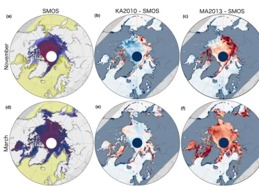
areas and will thus produce the same brightness temperatures using the same input data. Therefore here we only show the correction for MA2013. L-band brightness temperature vari-ations in Arctic open waters are low compared to sea ice and the difference between SMOS measurements and simulated brightness temperatures from the radiative transfer models should be less than 2 K, assuming temperatures around freez-ing point and 30 psu salinity (Berger et al., 2002).
We simulate brightness temperatures in all open water ar-eas north of 50◦ latitude. As a first step, we project the ORAP5 reanalysis on the polar-stereographic grid SMOS is using. Afterwards, we obtain a monthly average by calculat-ing brightness temperatures for each day of the month us-ing daily input data. Then, we average all brightness tem-peratures corresponding to a single day to a monthly value. We find an average bias of 4.5 K between MA2013 and the SMOS observations in November and March (Fig. 1). To identify the open water areas, we exclude all data points with a fractional sea ice coverage above zero in the ORAP5 re-analysis and also exclude all data points flagged as land, in either the reanalysis product or SMOS observations. Further-more, brightness temperatures of more than 120 K are con-sidered as outliers and are excluded as well. Finally, a total of 99085 data points show an average open water brightness temperature TBSMOS=100.7 K, whereas the models have an average of TBmodel=96.1 K.
To correct for the bias of open water areas we add the dif-ference of 4.5 K to the overall brightness temperature of sea-water. Subsequently, results of the radiative transfer models show the main accumulation of data points at around 99 K and a second, weaker one beginning at 99.5 K, each one with a tail towards higher brightness temperatures of SMOS. The wide range of observed brightness temperatures at 99 K is ex-plained by the complexity of nature and the simplicity of the radiative transfer model. As not all parameters are taken into account in the model, e.g., wind speed, the simulated bright-ness temperatures tend to be less diverse. The second tail at 99.5 K has evidence in the Baltic Sea. In that area, lower sea surface salinity and higher water temperature compared to the rest of the Arctic waters lead to higher brightness tem-peratures. However, this is not a general statement about the quality of the brightness temperatures above Arctic seawa-ter but a correction only for this analysis. The correction is used in all following simulations using the radiative transfer models.
2.5 Sea ice growth model
To obtain a reference point for Arctic sea ice thickness growth for the radiative transfer model sensitivity study in Sect. 3.2, we utilize an empirical sea ice growth model (Lebedev, 1938). The sea ice thickness increase is param-eterized byd=1.3320.58cm with the freezing days 2=
R
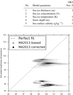
Table 1.Uncertainties of the ORAS5 reanalysis and monthly variations of the ORAP5 reanalysis for the radiative transfer model input parameters expressed as the 99 % quantile.
ORAS5 uncertainty ORAP5 monthly variation No. Model parameter Nov 2012 Mar 2013 Nov 2012 Mar 2013
1 Sea ice thickness (m) 0.24 0.17 0.76 0.87 2 Sea ice concentration (%) 4.4 8.1 97 69 3 Sea ice temperature (K) 0.31 0.87 18.5 18
4 Snow depth (m) 0.03 0.03 0.1 0.17
5 Sea surface salinity (g kg−1) 0.38 0.32 3.56 1.5
Figure 1. Seawater brightness temperature comparison between SMOS and MA2013. Contour lines (MA2013 biased) represent a direct comparison between simulated and measured brightness tem-perature above open seawater. Filled contours (MA2013 corrected) represent the same comparison but with a correction for simulated brightness temperatures of 4.5 K.
Ta(in◦C). The sea ice growth model has been used in var-ious prevvar-ious studies (e.g., Yu and Lindsay, 2003) and will provide an initial estimate of the sea ice thickness growth over a certain time period.
3 Results
3.1 Brightness temperature comparison
Brightness temperatures simulated with MA2013 are gener-ally higher than brightness temperatures of KA2010 by up to around 15 K (Fig. 2). The largest differences are located in the outer sea ice zones with the highest magnitude where sea ice concentration is close to 100 %, and an increase of sea ice thickness with time is expected, such as in the East Siberian
Sea or the Canadian Arctic Archipelago in November or the Sea of Okhotsk in March. For a first evaluation of the bright-ness temperature models, the two extreme cases of open wa-ter and 100 % multi-year thick sea ice can be considered. Since we already treated the lower boundary of open ocean brightness temperatures with a water bias correction as indi-cated above, we now concentrate on the upper boundary of a saturated signal over thick sea ice areas. We find higher simu-lated brightness temperatures in the central part of the Arctic by MA2013. The value in MA2013 saturates around∼255 K whereas KA2010 shows a maximum∼240 K. There are no indications for seasonal changes between brightness temper-atures from November and March except the increased area covered by sea ice. The variability in March shows a larger variation of brightness temperature difference close to the sea ice edge.
Brightness temperatures measured by SMOS appear to be in between the simulated ones of KA2010 and MA2013 in-fluenced by strong spatial differences (Fig. 3). In Novem-ber 2012, both models show higher brightness tempera-tures in the East Siberian Sea and the Canadian Arctic Archipelago. Lower brightness temperatures are located in the Canadian Basin and the Chukchi Sea with extension to the Bering Street. A different picture is shown in the cen-tral Arctic at grid points with more than 80 % sea ice con-centration coverage, where both models simulate brightness temperatures with deviations of opposite directions. In this area, the model of KA2010 shows lower (−2.4±7.3 K) and MA2013 higher (9.4±7.5 K) brightness temperatures com-pared to SMOS observations in November 2012. The same is true for March 2013, although KA2010 (0.3±7.1 K) shows a stronger agreement in the central Arctic than MA2013 (10.8±7.1 K). Brightness temperature deviations between KA2010 and the SMOS measurements show a higher vari-ability between positive and negative differences. MA2013 appears to be positively biased not only in November 2012 but in March 2013 as well. The simulations exceed SMOS brightness temperatures almost everywhere in the Arctic with deviations up to 20 K in the Labrador Sea and Sea of Okhotsk.
Figure 2.Monthly brightness temperatures simulated by KA2010 (aandd) and MA2013 (bande). Panels(a)–(c)show the November 2012 brightness temperature distribution based on ORAP5 reanalysis input data with a comparison plot of both models at(c). Panels(d)–(f)are equal, but for March 2013.
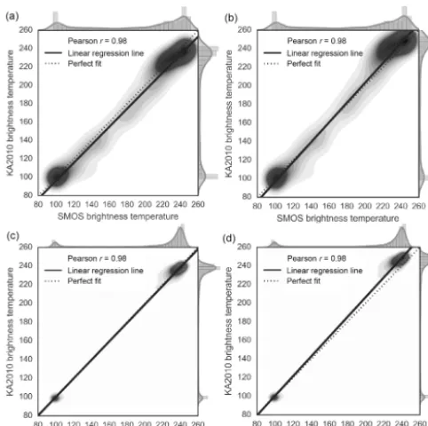
Figure 4. Brightness temperature comparison between simulated and observed brightness temperatures in November 2012 (aand b) and March 2013 (candd) for KA2010 (aandc) and MA2013 (b andd). The Pearson correlationr between simulated and ob-served brightness temperatures over sea ice for MA2013 and KA2010, respectively, is stated in the legend.
are clustered at 105±3 and 240±7 K (Fig. 4). The latter is associated with thicker sea ice related to saturated bright-ness temperatures at 1.4 GHz. Simulated brightbright-ness temper-ature shows a high correlation of the distribution state of
r=0.98 or r=0.97 with SMOS measurements. KA2010 brightness temperatures are on average 2 K lower than SMOS in November, whereas MA2013 simulates larger brightness temperatures in thick ice regions in March and November. Furthermore, as already seen in Fig. 3, MA2013 overesti-mates brightness temperatures above∼190 K also in March. The difference between simulated and observed brightness temperatures is largest in between the main clusters, although most points appear to concentrate around the 1:1 line.
3.2 Radiative transfer model sensitivity study
In order to identify the most important input variables for the radiative transfer models, we evaluate the sensitivity of the models to certain changes of sea ice, snow and seawater pa-rameters. We keep all but one parameter fixed at a monthly value and calculate the brightness temperatures for the min-imum and the maxmin-imum simulated value within the month for one physical parameter. That will give us two different brightness temperatures – one for the minimum and one for the maximum – of which the difference is the range of bright-ness temperature change related to one of the parameters
Figure 5.Most influential physical variables from ORAP5 on the brightness temperature gradient. Monthly values are shown for November 2012(a–b) and March 2013(c–d)for KA2010 (a–c) and MA2012(b–d).
that can be expected. Varying all input parameters provided by the ORAP5 reanalysis, we quantify the impact of certain physical parameters on our brightness temperatures at a spe-cific place over the time span of 1 month.
Figure 6.Freeze-up event in October to November 2012 that took place in the Laptev Sea (77.5◦N, 137.5◦E). Brightness temperature time series of from KA2010, MA2013 and SMOS measurements (top) and sea ice thickness and concentration time series of ORAP5, ASI and Lebedev retrieval model data (bottom).
it appears that sea surface temperature dominates (7 %). The sea surface salinity only contributes in very small areas in the Fram Strait, where the sea surface temperature and salin-ity are higher (<1 %).
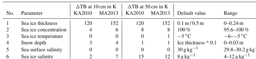
The propagating errors from ORAP5 uncertainties to the brightness temperature simulations are shown in Table 2. Similar to the method used in Fig. 5 one parameter varies over a range of values whereas all other parameters are fixed to a default value. The range of values is set to be the ORAS5 monthly uncertainty of November (Table 1). At that time, the sea ice thickness uncertainty is higher than in March as it is in the middle of the sea ice growth season. This calculation is performed twice, once for thin sea ice (10 cm) and once for a thick sea ice (50 cm) (except in the case of varying sea ice thickness). For both sea ice thickness values, the ORAP5 sea ice thickness uncertainty of 24 cm dominates the simu-lated brightness temperature signal with a value up to 152 K in MA2013. The influence of all other physical properties do not exceed more than 8 K except the sea ice salinity with val-ues up to 15 K. The effect of the sea ice temperature and sea surface salinity vanishes in this case of thin sea ice.
For a more detailed analysis on the contribution of sea ice thickness and concentration to the modeled brightness temperatures, a sample freeze-up situation is investigated at a point located in the Laptev Sea (77.5◦N, 137.5◦E) from October to November 2012 (Fig. 6). The observational sea ice concentration product ASI (ARTIST Sea Ice algorithm) (Kaleschke et al., 2001; Spreen et al., 2008) shows a rapid freeze-up to 80 % sea ice coverage in just a few days. The brightness temperatures of SMOS measurements and the KA2010 and MA2013 models show high agreement with some exceptions on the first days of the freezing period, which starts around the 25 October. The simulated
bright-ness temperatures appear to underestimate the SMOS mea-surements at the beginning of the season, which leads to a more linear brightness temperature increase rather than a log-arithmic shape as observed from the SMOS measurements. However, the simulated sea ice concentration of ORAP5 is lower than the observed ASI sea ice concentration and needs almost 2 weeks to catch up to the same coverage as ASI. The sea ice thickness, in contrast, shows a fast thickening to more than half a meter even before the main freeze-up event takes place. The sea ice growth model of Lebedev (1938) accumulates sea ice as a function of the temperature differ-ence between the surface air temperature and freezing point of water as well as the number of freezing days below zero degrees. In contrast to the sea ice thickness of ORAP5, Lebe-dev’s parameterization shows a gradual increase of ice thick-ness throughout the freeze-up event. Following, we observe an underestimation of sea ice concentration and an overes-timation of sea ice thickness in the reanalysis over a range of 2 weeks, whereas the SMOS brightness temperature only deviate more than 20 K for 5 days.
4 Discussion
Our results indicate that brightness temperature differences up to around 15 K, and even higher differences at the ice edge, can be due to the usage of different radiative transfer models (Fig. 2). Even though both models tend to have the same signatures, KA2010 shows lower brightness tempera-tures than the MA2013 in the whole Arctic. This was ex-pected as the MA2013 model is able to take multiple sea ice layers into account, as well as the radiometric effect of snow on top of sea ice, whereas KA2010 only indirectly includes the effect of snow with the representation of the thermo-dynamic insulation effect. However, compared with SMOS brightness temperatures, it appears that MA2013 driven with the ORAP5 output overestimates brightness temperatures in many parts of the Arctic, most pronouncedly in March in the central Arctic region. This area is mostly covered by thick sea ice. In contrast, KA2010 shows good agreement in the central Arctic area.
rea-Table 2.Changes of simulated brightness temperatures in KA2010 and MA2013 related to alternating physical parameters. The range is based on the ORAS5 uncertainties of November (Table 1). Two cases of thin sea ice (10 cm) and thicker sea ice (50 cm) are shown.
1TB at 10 cm in K 1TB at 50 cm in K
No. Parameter KA2010 MA2013 KA2010 MA2013 Default value Range
1 Sea ice thickness 120 152 120 152 0.1 m / 0.5 m 0–0.24 m 2 Sea ice concentration 4 6 8 8 100 % 95.6–100 % 3 Sea ice temperature 0 0 0 1 −5◦C −6–−5◦C 4 Snow depth 3 4 1 1 Ice thickness * 0.1 0–0.03 m 5 Sea surface salinity 0 0 0 0 30 g kg−1 29.8–30.2 g kg−1 6 Sea ice salinity 2 7 15 12 8 g kg−1 4–12 g kg−1
sons are as follows. (1) The brightness temperature differ-ence between ice and water is higher for thicker ice, thus a changing ice concentration changes the mixture’s brightness temperature more than for thinner ice. (2) Due to the lower sensitivity of the L-band signal to ice thickness for thicker ice, the brightness temperature difference induced by chang-ing ice concentration leads to a higher ice thickness differ-ence for thicker ice than for thinner ice.
Here, we provide sea ice fractional coverage from our re-analysis to the radiative transfer models and are thus able to reduce the uncertainty of sea ice fraction changes compared to studies with an assumption of a constant 100 % sea ice concentration coverage (Table 2) (Tian-Kunze et al., 2014).
At a sea ice thickness of around 50 cm, an uncertainty of 5 % fractional sea ice coverage accounts for a difference of 8 K (Kaleschke et al., 2010), which in turn can result in a sea ice thickness uncertainty of more than 10 cm. In occasional events, the deviation of sea ice concentration from the reanal-ysis data to the here-investigated ASI sea ice concentration can be even higher, with differences up to 40 % (Fig. 6). The largest error is due to the sea ice thickness with an estimated uncertainty of 24 cm for ORAP5 in November 2012, corre-sponding to a brightness temperature difference of 120 and 152 K for thin ice (below 24 cm) in KA2010 or MA2013, respectively. This uncertainty is more than 10 times higher than all other uncertainties in the case of typical first-year sea ice represented by the default values in Table 2, with the exception of sea ice salinity, which is a function of sea ice thickness and sea surface salinity (Ryvlin, 1974). This is ben-eficial for assimilation purposes as 93 % in MA2013 or 90 % in KA2010 of all brightness temperature deviations between SMOS and the radiative transfer models are rooted in the sea ice thickness (compare Table 2).
In order to assimilate thin sea ice thickness it is crucial to understand the impact of all physical parameters on the brightness temperature simulations. Kaleschke et al. (2012) found sea ice concentration and thickness changes in thin sea ice areas are the most important variables for L-band bright-ness temperatures. We here support this evidence as our most dominating dependencies for brightness temperature simula-tions are found to be the same throughout the Arctic (Fig. 5).
Over thick sea ice in the central Arctic we find the sea ice and/or snow surface temperature to be the most influential parameter. Since sea ice concentration is close to 100 % and sea ice thickness is above the L-band sensitivity, brightness temperature changes are due to the impact of snow depth and sea ice and/or snow temperature changes that come with it. In thin sea ice regions, variations of sea ice temperature, snow depth and sea surface salinity can have an accumulated influ-ence of up to more than 25 K (not shown).
Our results also show a significant influence of sea surface temperature and salinity in areas of thin sea ice close to the ice edge. This is explained by a fractional sea ice coverage of less than 10 %, where brightness temperature variations are dominated by changing open water emissivities. We point out that sea surface temperature and salinity get more important in regions with lower sea ice coverage. Therefore, in the case that partially ice-covered areas are taken into account we cau-tion that a climatology of sea surface temperature or salinity might not be sufficient enough to picture the transition be-tween open water towards the sea ice edge. This is especially true for the declining sea ice observed in the recent years as the sea ice edge is likely to be located at a different location than in the previous years.
order to determine reasonable areas for brightness tempera-ture assimilation in that KA2010 in March agrees most. We specifically concentrate on the saturated case, as it is next to water the only reliable reference point we can address for a quality assessment of the models. Thus, based on ORAP5 reanalysis input data and electromagnetic formulations used here, we suggest using the KA2010 radiative transfer model for brightness temperature assimilation. However, for the re-maining 8 % of all simulated data points with intermediate sea ice thickness and concentration we are unable to find a favorable radiative transfer model as the results of the models are superimposed by the sea ice thickness uncertainty. Note that this is not a statement about the quality of the radiation model in general but rather a suggestion for the specific as-sumptions and characteristics of the LIM2 sea ice models that were used in this study.
Although the statistical representation of brightness tem-peratures is well captured, we find large discrepancies in times of rapid sea ice changes (Fig. 6). For an example case, ORAP5 appears to have difficulties simulating freeze-up events, in which we see an overestimation of sea ice thick-ness and an underestimation of sea ice concentration. The assimilation of OSI-SAF sea ice concentration into ORAP5 pushes the sea ice concentration into the right direction but appears to be too slow to picture changes in a short period of time. A smaller fractional sea ice concentration and an over-estimation of sea ice thickness then lead to simulated bright-ness temperatures that fit with observed SMOS brightbright-ness temperatures, even though both parameters are divergent at this time.
5 Summary and conclusion
For the direct assimilation of satellite measurements, in this case brightness temperatures, it is necessary to generate a modeled first guess using the output from a numerical model and a forward/observation operator to translate geophysical variables into measurement space. We tested the approach using simulations from ORAP5 and two radiative transfer models to compute L-band brightness temperatures. These simulations were then compared against actual SMOS ob-servations. This is normally the first step in a data assim-ilation framework, often referred to as monitoring of first-guess departures. We used the radiative transfer models from Kaleschke et al. (2010) (denoted as KA2010) and Maaß et al. (2013) (MA2013) and focused on the winter season 2012/2013, namely November 2012 and March 2013, ac-counting for the start and the end of the winter season, re-spectively.
The results of this study indicate that both radiative trans-fer models are able to simulate Arctic-wide brightness tem-peratures with realistic spatial and temporal variability, e.g., we are able to observe a similar increase of simulated and observed brightness temperatures from thin to thicker sea ice
areas. Although both models show a decent fit in November, the model of Maaß et al. (2013) tends to overestimate bright-ness temperatures in the saturated case of thick sea ice in March with the configurations applied here. A Kolmogorov– Smirnov test thus only accepts the brightness temperature distribution of KA2010 in March by taking the SMOS ob-servation as the reference probability distribution. All oth-ers, especially the results of MA2013 in March, are rejected. For starting the integration of SMOS measurements into the ORAP5 data assimilation system we therefore suggest using the model of KA2010 for a brightness temperature assimi-lation into the ORAP5 reanalysis project. This suggestion is primarily based on a comparison between SMOS and sim-ulated brightness temperatures over thick sea ice and open water and does not make a statement about the ability of the model to reproduce brightness temperatures in thin sea ice conditions.
By analyzing the sensitivity of the brightness temperatures with respect to geophysical parameters, we expect the largest impact of SMOS observations in the marginal ice zone. Here, the most important parameters are the sea ice thickness and fractional sea ice coverage. This result supports the findings of other studies (e.g., Kaleschke et al., 2012). In thicker sea ice areas the dominant parameter is the sea surface temper-ature since the sea ice fractional coverage is close to 100 % and sea ice thickness changes do not affect the measurements at 1.4 GHz. The influence of the sea ice temperature, snow depth and sea ice salinity increases in thinner sea ice areas but will still be less than the sea ice thickness and concentra-tion. However, the smaller the fractional sea ice coverage is, the more important the sea surface temperature and salinity become. This becomes relevant at sea ice concentration be-low 15 %, usually found in small regions at the very outer sea ice edge.
Even though the sea ice thickness and concentration in ORAP5 are partly constrained by observations (Tietsche et al., 2015), the model shows difficulties representing a rapid freeze-up event with an underestimation of sea ice concentra-tion and an overestimaconcentra-tion of sea ice thickness. However, the corresponding resulting brightness temperatures are in agree-ment with the SMOS observations.
It is therefore strongly recommended to assimilate bright-ness temperature measurements from 6 to 37 GHz simultane-ously with L-band measurements constraining fractional sea ice coverage and thickness consistently at the same time. The observation operators will become available together with an observational data set spanning almost a decade. Never-theless, more collocated in situ or laboratory measurements of ice and snow parameters and multi-frequency brightness temperature are needed to advance our understanding of ra-diative transfer modeling.
measurements such as brightness temperatures or radiances rather than a set of individually retrieved geophysical has a number of advantages:
– The first guess in observation space is based on a consis-tent set of input data. This ensures that the observation errors for the different measurements remain uncorre-lated and are fully traceable to the instrument error. It is also ensured that the same observation is only used once.
– Systematic differences between the modeled first guess and the individual measurements can be treated consis-tently and a bias correction scheme can be included in the data assimilation scheme.
– Processing measurements at their native resolution al-lows a better characterization of the representativity er-ror, which accounts for the different spatial and tempo-ral support of the model and the observations.
– The quality control and data thinning can be done con-sistently in observation space, addressing the error cor-relations in the original measurements. In addition, in situ measurements remain independent information that can be either assimilated in the analysis or used for val-idation purposes or for calibrating the model or the for-ward operator.
– Finally, the Jacobians can be used in the analysis to de-termine the relative weight of the observations.
Adjusting the existing systems for the direct assimilation of measurements is a substantial task and requires dedicated ad-ditional investments in manpower and money. However, the assimilation of brightness temperatures will eventually result in more accurate and consistent analyses of the true state of Arctic sea ice at any given time.
Data availability. L3B brightness temperatures are provided by the CliSAP Integrated Climate Data Center (ICDC) on http://icdc.cen. uni-hamburg.de/1/daten/cryosphere/l3b-smos-tb.html (Tian-Kunze et al., 2012). The reanalysis data of ORAP5 were kindly pro-vided by ECMWF. The ORAS5 uncertainties will be soon available at http://www.ecmwf.int/en/research/climate-reanalysis/ browse-reanalysis-datasets (ECMWF, 2018).
Competing interests. The authors declare that they have no conflict of interest.
Acknowledgements. We thank Steffen Tietsche for the provision of ORAP5 reanalysis data and fruitful discussions and Andreas Wernecke, who helped to implement the cosmic and galactic background radiation representation. We thank the “Science Snack” team for fruitful discussions. The work was funded by ESA
and Deutsche Forschungsgemeinschaft (DFG EXC177).
Edited by: Julienne Stroeve
Reviewed by: two anonymous referees
References
Berger, M., Camps, A., Font, J., Kerr, Y., Miller, J., Johannessen, J., Boutin, J., Drinkwater, M. R., Skou, N., Floury, N., Rast, M., Rebhan, H., and Attema, E.: Measuring ocean salinity with ESA’s SMOS mission – Advancing the science, Esa Bulletin-European Space Agency, 113–121, 2002.
Bouillon, S., Morales Maqueda, M. A., Legat, V., and Fichefet, T.: An elastic-viscous-plastic sea ice model formulated on Arakawa B and C grids, Ocean Modell., 27, 174–184, https://doi.org/10.1016/j.ocemod.2009.01.004, 2009.
Burke, W. J., Schmugge, T., and Paris, J. F.: Comparison of 2.8-and 21-cm microwave radiometer observations over soils with emission model calculations, J. Geophys. Res., 84, 287–294, https://doi.org/10.1029/JC084iC01p00287, 1979.
Chen, Z., Liu, J., Song, M., Yang, Q., and Xu, S.: Impacts of As-similating Satellite Sea Ice Concentration and Thickness on Arc-tic Sea Ice Prediction in the NCEP Climate Forecast System, J. Climate, 30, 8429–8446, https://doi.org/10.1175/JCLI-D-17-0093.1, 2017.
Day, J., Hawkins, E., and Tietsche, S.: Will Arctic sea ice thickness initialization improve seasonal forecast skill?, Geophys. Res. Lett., 41, 7566–7575, https://doi.org/10.1002/2014GL061694, 2014.
Dee, D. P., Uppala, S. M., Simmons, A. J., Berrisford, P., Poli, P., Kobayashi, S., Andrae, U., Balmaseda, M. A., Balsamo, G., Bauer, P., Bechtold, P., Beljaars, A. C. M., van de Berg, L., Bid-lot, J., Bormann, N., Delsol, C., Dragani, R., Fuentes, M., Geer, A. J., Haimberger, L., Healy, S. B., Hersbach, H., Hólm, E. V., Isaksen, L., Kållberg, P., Köhler, M., Matricardi, M., McNally, A. P., Monge-Sanz, B. M., Morcrette, J.-J., Park, B.-K., Peubey, C., de Rosnay, P., Tavolato, C., Thépaut, J.-N., and Vitart, F.: The ERA-Interim reanalysis: configuration and performance of the data assimilation system, Q. J. Roy. Meteorol. Soc., 137, 553– 597, https://doi.org/10.1002/qj.828, 2011.
Dinnat, E. P., Boutin, J., Caudal, G., and Etcheto, J.: Is-sues concerning the sea emissivity modeling at L band for retrieving surface salinity, Radio Sci., 38, 8060, https://doi.org/10.1029/2002RS002637, 2003.
ECMWF: ORAS uncertainties, available at: https://www.ecmwf. int/en/forecasts/datasets/browse-reanalysis-datasets, last access: 8 March, 2018.
Gabarro, C., Turiel, A., Elosegui, P., Pla-Resina, J. A., and Porta-bella, M.: New methodology to estimate Arctic sea ice concentra-tion from SMOS combining brightness temperature differences in a maximum-likelihood estimator, The Cryosphere, 11, 1987– 2002, https://doi.org/10.5194/tc-11-1987-2017, 2017.
Kaleschke, L., Lüpkes, C., Vihma, T., Haarpaintner, J., Bochert, A., Hartmann, J., and Heygster, G.: SSM/I sea ice remote sensing for mesoscale ocean-atmosphere interaction analysis, Can. J. Re-mote Sens., 27, 526–537, 2001.
for 1.4 GHz radiometry and application to airborne measure-ments over low salinity sea-ice, The Cryosphere, 4, 583–592, https://doi.org/10.5194/tc-4-583-2010, 2010.
Kaleschke, L., Tian-Kunze, X., Maaß, N., Mäkynen, M., and Dr-usch, M.: Sea ice thickness retrieval from SMOS brightness tem-peratures during the Arctic freeze-up period, Geophys. Res. Lett., 39, L05501, https://doi.org/10.1029/2012GL050916, 2012. Kaleschke, L., Tian-Kunze, X., Maaß, N., Beitsch, A., Wernecke,
A., Miernecki, M., Müller, G., Fock, B. H., Gierisch, A. M., Schlünzen, K. H., Pohlmann, T., Dobrynin, M., Hendricks, S., Asseng, J., Gerdes, R., Jochmann, P., Reimer, N., Holfort, J., Melsheimer, C., Heygster, G., Spreen, G., Gerland, S., King, J., Skou, N., Søbjærg, S. S., Haas, C., Richter, F., and Casal, T.: SMOS sea ice product: Operational application and validation in the Barents Sea marginal ice zone, Remote Sens. Environ., 180, 264–273, https://doi.org/10.1016/j.rse.2016.03.009, 2016. Kalnay, E., Kanamitsu, M., Kistler, R., Collins, W., Deaven,
D., Gandin, L., Iredell, M., Saha, S., White, G., Woollen, J., Zhu, Y., Chelliah, M., Ebisuzaki, W., Higgins, W., Janowiak, J., Mo, K. C., Ropelewski, C., Wang, J., Leet-maa, A., Reynolds, R., Jenne, R., and Joseph, D.: The NCEP/NCAR 40-Year Reanalysis Project, B. Am. Meteorol. Soc., 77, 437–472, https://doi.org/https://doi.org/10.1175/1520-0477(1996)077<0437:TNYRP>2.0.CO;2, 1996.
Kerr, Y. H., Waldteufel, P., Wigneron, J. P., Martinuzzi, J. M., Font, J., and Berger, M.: Soil moisture retrieval from space: The Soil Moisture and Ocean Salinity (SMOS) mission, IEEE T. Geosci. Remote, 39, 1729–1735, https://doi.org/10.1109/36.942551, 2001.
Klein, L. and Swift, C.: An improved model for the di-electric constant of sea water at microwave frequencies, Oceanic Engineering, IEEE J. Ocean. Eng., 2, 104–111, https://doi.org/10.1109/joe.1977.1145319, 1977.
Laxon, S. W., Giles, K. A., Ridout, A. L., Wingham, D. J., Willatt, R., Cullen, R., Kwok, R., Schweiger, A., Zhang, J., Haas, C., Hendricks, S., Krishfield, R., Kurtz, N., Far-rell, S., and Davidson, M.: CryoSat-2 estimates of Arctic sea ice thickness and volume, Geophys. Res. Lett., 40, 732–737, https://doi.org/10.1002/grl.50193, 2013.
Lebedev: Rost l’da v arkticheskikh rekakh i moriakh v zavisimosti ot otritsatel’nykh temperatur vozdukha, 5–6 Edn., 1938. Lindsay, R. and Schweiger, A.: Arctic sea ice thickness loss
deter-mined using subsurface, aircraft, and satellite observations, The Cryosphere, 9, 269–283, https://doi.org/10.5194/tc-9-269-2015, 2015.
Maaß, N., Kaleschke, L., Tian-Kunze, X., and Drusch, M.: Snow thickness retrieval over thick Arctic sea ice using SMOS satellite data, The Cryosphere, 7, 1971–1989, https://doi.org/10.5194/tc-7-1971-2013, 2013.
Maaß, N., Kaleschke, L., Tian-Kunze, X., and Tonboe, R. T.: Snow thickness retrieval from L-band brightness tem-peratures: a model comparison, Ann. Glaciol., 56, 9–17, https://doi.org/10.3189/2015AoG69A886, 2015.
Maykut, G. A.: The Surface Heat and Mass Balance, 395–463, in collection, The Geophysics of Sea Ice, Editor Norbert Un-tersteiner, Springer Science+Business Media New York eBook, ISBN 978-1-4899-5352-0, https://doi.org/10.1007/978-1-4899-5352-0, 1195 pp., 1986.
Mecklenburg, S., Drusch, M., Kerr, Y. H., Font, J., Martin-Neira, M., Delwart, S., Buenadicha, G., Reul, N., Daganzo-Eusebio, E., and Oliva, R.: ESA’s Soil Moisture and Ocean Salinity Mission – Mission overview and first results, Geophys. Res. Abstract., 13, 3628–3628, 2012.
Meier, W. N., Hovelsrud, G. K., van Oort, B. E. H., Key, J. R., Ko-vacs, K. M., Michel, C., Haas, C., Granskog, M. A., Gerland, S., Perovich, D. K., Makshtas, A., and Reist, J. D.: Arctic sea ice in transformation: A review of recent observed changes and impacts on biology and human activity, Rev. Geophys., 52, 185– 217, https://doi.org/10.1002/2013RG000431, 2014.
Menashi, J. D., St Germain, K. M., Swift, C., Comiso, J. C., and Lo-hanick, A.: Low-frequency passive-microwave observations of sea ice in the Weddell Sea., J. Geophys. Res.-Oceans, 98, 22569– 22577, 1993.
Peng, G., Meier, W. N., Scott, D. J., and Savoie, M. H.: A long-term and reproducible passive microwave sea ice concentration data record for climate studies and monitoring, Earth Syst. Sci. Data, 5, 311–318, https://doi.org/10.5194/essd-5-311-2013, 2013. Ricker, R., Hendricks, S., Kaleschke, L., Tian-Kunze, X., King, J.,
and Haas, C.: A weekly Arctic sea-ice thickness data record from merged CryoSat-2 and SMOS satellite data, The Cryosphere, 11, 1607–1623, https://doi.org/10.5194/tc-11-1607-2017, 2017. Ryvlin, A. I.: Method of forecasting flexural strength of an ice
cover, Probl. Arct. Antarct, 45, 79–86, 1974.
Sachs, L. and Hedderich, J.: Angewandte Statistik, Springer, p. 338, 2006.
Sakov, P., Counillon, F., Bertino, L., Lisaeter, K. A., Oke, P. R., and Korablev, A.: TOPAZ4: an ocean-sea ice data assimilation system for the North Atlantic and Arctic, Ocean Sci., 8, 633– 656, https://doi.org/10.5194/os-8-633-2012, 2012.
Semtner, A.: A model for the thermodynamic growth of sea ice in numerical investigations of climate, J. Phys. Ocean., 6, 379–389, 1976.
Simmons, A., Fellous, J.-L., Ramaswamy, V., Trenberth, K., and Res, S. T. C. S.: Observation and integrated Earth-system sci-ence: A roadmap for 2016–2025, Adv. Space Res., 57, 2037– 2103, https://doi.org/10.1016/j.asr.2016.03.008, 2016.
Spreen, G., Kaleschke, L., and Heygster, G.: Sea ice remote sens-ing ussens-ing AMSR-E 89-GHz channels, J. Geophys. Res., 113, C02S03, https://doi.org/10.1029/2005JC003384, 2008.
Stark, J. D., Ridley, J., Martin, M., and Hines, A.: Sea ice concentration and motion assimilation in a sea ice-ocean model, J. Geophys. Res.-Oceans, 113, 1–19, https://doi.org/10.1029/2007JC004224, 2008.
Tian-Kunze, X., Kaleschke, L., and Maass, N.: SMOS Daily Po-lar Gridded Brightness Temperatures, [2012–2013], available at: icdc.cen.uni-hamburg.de (last access: 8 March 2018), 2012. Tian-Kunze, X., Kaleschke, L., Maaß, N., Mäkynen, M., Serra, N.,
Drusch, M., and Krumpen, T.: SMOS-derived thin sea ice thick-ness: algorithm baseline, product specifications and initial verifi-cation, The Cryosphere, 8, 997–1018, https://doi.org/10.5194/tc-8-997-2014, 2014.
Tietsche, S., Balmaseda, M. A., Zuo, H., and Mogensen, K.: Arctic sea ice in the global eddy-permitting ocean reanalysis ORAP5, Clim. Dynam., 49, 775–789, https://doi.org/10.1007/s00382-015-2673-3, 2015.
Ulaby, F. T., Moore, R. K., and Fung, A. K.: Microwave remote sensing. Active and passive, Kansas Univ., Lawrence, KS, United States, 1981.
Vikhamar-Schuler, D., Isaksen, K., Haugen, J. E., Tommervik, H., Luks, B., Vikhamar-Schuler, T., and Bjerke, J. W.: Changes in Winter Warming Events in the Nordic Arctic Region, J. Climate, 29, 6223–6244, https://doi.org/10.1175/JCLI-D-15-0763.1, 2016.
Warren, S. G., Rigor, I. G., Untersteiner, N., Radionov, V. F., Bryazgin, N. N., Aleksandrov, Y. I., and Colony, R.: Snow Depth on Arctic Sea Ice, J. Cli-mate, 12, 1814–1829, https://doi.org/10.1175/1520-0442(1999)012<1814:SDOASI>2.0.CO;2, 1999.
Xie, J., Counillon, F., Bertino, L., Tian-Kunze, X., and Kaleschke, L.: Benefits of assimilating thin sea ice thickness from SMOS into the TOPAZ system, The Cryosphere, 10, 2745–2761, https://doi.org/10.5194/tc-10-2745-2016, 2016.
Yang, Q., Losa, S., Losch, M., Tian-Kunze, X., Nerger, L., Liu, J., Kaleschke, L., and Zhang, Z.: Assimilating SMOS sea ice thickness into a coupled ice-ocean model using a local SEIK filter, J. Geophys. Res., 119, 6680–6692, https://doi.org/10.1002/2014JC009963, 2014.
Yu, Y. and Lindsay, R. W.: Comparison of thin ice thick-ness distributions derived from RADARSAT Geophys-ical Processor System and advanced very high resolu-tion radiometer data sets, J. Geophys. Res., 108, 3387, https://doi.org/10.1029/2002JC001319, 2003.