www.atmos-meas-tech.net/8/729/2015/ doi:10.5194/amt-8-729-2015
© Author(s) 2015. CC Attribution 3.0 License.
A six-beam method to measure turbulence statistics using
ground-based wind lidars
A. Sathe, J. Mann, N. Vasiljevic, and G. Lea
DTU Wind Energy, Risø campus, Roskilde, Denmark Correspondence to: A. Sathe ([email protected])
Received: 22 September 2014 – Published in Atmos. Meas. Tech. Discuss.: 10 October 2014 Revised: 4 January 2015 – Accepted: 19 January 2015 – Published: 12 February 2015
Abstract. A so-called six-beam method is proposed to mea-sure atmospheric turbulence using a ground-based wind li-dar. This method requires measurement of the radial velocity variances at five equally spaced azimuth angles on the base of a scanning cone and one measurement at the centre of the scanning circle, i.e.using a vertical beam at the same height. The scanning configuration is optimized to minimize the sum of the random errors in the measurement of the second-order moments of the components (u, v, w) of the wind field. We present this method as an alternative to the so-called veloc-ity azimuth display (VAD) method that is routinely used in commercial wind lidars, and which usually results in signif-icant averaging effects of measured turbulence. In the VAD method, the high frequency radial velocity measurements are used instead of their variances. The measurements are per-formed using a pulsed lidar (WindScanner), and the derived turbulence statistics (using both methods) such as theuandv variances are compared with those obtained from a reference cup anemometer and a wind vane at 89 m height under dif-ferent atmospheric stabilities. The measurements show that in comparison to the reference cup anemometer, depending on the atmospheric stability and the wind field component, the six-beam method measures between 85 and 101 % of the reference turbulence, whereas the VAD method measures be-tween 66 and 87 % of the reference turbulence.
1 Introduction
Wind lidars are being used significantly for wind energy ap-plications. They measure mean wind speeds with great accu-racy, and are very useful tools in the measurement of wind profiles (Smith et al., 2006; Kindler et al., 2007; Peña et al.,
2009; Wagner et al., 2011). New recommended practices are being defined for wind resource assessments (Clifton et al., 2013). However their use in measuring atmospheric turbu-lence has not yet been established, particularly with the com-mercial lidars (Sathe et al., 2011b). The main reason is that for a commercial lidar, the measured lidar data is processed using the so-called velocity azimuth display (VAD) method, where the measurements of the radial velocity (also called the line-of-sight velocity) at different azimuth angles are combined to deduce the wind field components. For the mean wind speed estimation, the VAD method produces negligible errors. For turbulence statistics the VAD method produces significant systematic errors (Sathe et al., 2011b; Sathe and Mann, 2012) mainly due to two reasons; one is the filtering of the smaller scales due to the large size of the probe volume within which the radial velocity is measured, and second is the contamination by the two-point correlation between the components of the wind field.
azimuth angles and one elevation angle, or by using only two lidar beams (Mann et al., 2010). In the present work, six beams are used, five at an elevation angle of 45◦and one vertical that enable us to also deduce the variances.
The ideas to measure turbulence using remote sensing in-struments have evolved, albeit slowly, since the pioneering works on radar meteorology (Lhermitte, 1962; Browning and Wexler, 1968). Based on the VAD scanning, Lhermitte (1969) was the first (to our knowledge) to suggest a tech-nique of deducing turbulence using the measurements of the variance of the radial velocity. Subsequently Wilson (1970) was the first to conduct an experiment using a pulsed Doppler radar and deducing turbulence in the convective boundary layer (0.1–1.3 km). Only turbulence scales larger than the pulse volume but smaller than the scanning circle could be measured since all the data from a single scan was used. Also, no comparison with any reference instrument was car-ried out, and hence, the reliability of the radar measurements could not be verified. Kropfli (1986) extended the study of Wilson (1970) to also include the turbulence scales larger than the scanning circle by using the data from multiple scans. Although the method was developed for Doppler radar studies, it could also be used for Doppler lidar studies. Eber-hard et al. (1989) was the first to perform turbulence stud-ies using a lidar following the methods of Wilson (1970); Kropfli (1986). Gal-Chen et al. (1992) also used the variances of the radial velocities to deduce turbulence, but with a dif-ferent scanning configuration. In all of the aforementioned studies with a Doppler lidar (or radar), the probe length was quite significant (of the order of 100 m), which perhaps was the reason to restrict these studies to the convective bound-ary layer. However if the turbulence measurements were de-sired close to the ground then they would be subjected to a significant amount of probe volume averaging. It was per-haps this reason that the focus on turbulence research with lidars shifted to understanding the probe volume averaging effect and providing potential solutions to compensate for it (Frehlich, 1994, 1997; Frehlich et al., 1994, 1998, 2006, 2008; Frehlich and Cornman, 2002; Frehlich and Kelley, 2008; Banakh et al., 1995a, b, 1996, 1999, 2010; Banakh and Smalikho, 1997a, b; Banakh and Werner, 2005; Sma-likho, 1995; Smalikho et al., 2005; Mann et al., 2010; Bran-lard et al., 2013). Even with the development of the modern lidar systems, where the probe lengths have shrunk to about 30 m for a pulsed lidar, significant amount of averaging still remains in the turbulence measurements within the surface layer, where the wind turbines operate (Mann et al., 2009, 2010; Sjöholm et al., 2009; Sathe et al., 2011b; Sathe and Mann, 2012). A detailed review of the state of the art with re-spect to turbulence measurements using ground-based wind lidars can be found in Sathe and Mann (2013).
Unfortunately within the wind energy sector, turbulence measurements are being deduced using the VAD scanning method, which results in a significant amount of filtering of turbulence, and contamination by the two-point
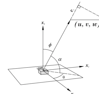
correla-Figure 1. Coordinate system of a lidar.
tion between the components of the wind field (Sathe et al., 2011b). In this work we attempt to significantly improve the turbulence measurements compared to those obtained by the VAD method, by extending the previously developed ideas of using the radial velocity variances (Lhermitte, 1969; Wil-son, 1970; Kropfli, 1986; Eberhard et al., 1989; Mann et al., 2010), but restricting them to using only six beams.
The structure of this article is divided into the follow-ing sections. Section 2 gives a detailed explanation of the six-beam technique. The optimum six-beam configuration, which is one of the main contributions of this article is also described in detail. In order to verify our method, turbulence measurements using the pulsed lidar WindScanner were per-formed and compared with a reference cup anemometer at a height of 89 m. The site description for the measurements is given in Sect. 3, whereas the results are described in Sect. 4. Discussions and conclusions are made in Sects. 5 and 6, re-spectively.
2 Theory of six-beam configuration
The instantaneous velocity field is characterized as a vector v=(u, v, w), and turbulence is characterized as the compo-nents of the Reynolds stress tensor,
R=
D
u02E
u0v0
u0w0
v0u0 Dv02E v0w0
w0u0 w0v0 Dw02E
, (1)
As shown in Fig. 1, at a given instant of time if we as-sume that a lidar measures at a point, and that the lidar beam is inclined at a certain zenith angleφ(in some literature the complement ofφis used, which is called as the elevation an-gleα=90◦−φ) from the vertical axis, and makes an azimuth angleθwith respect to the axes in the horizontal plane, then the radial velocity (also called as the line-of-sight velocity) can be mathematically written as,
vr(φ, θ, df)=n(φ, θ )·v(n(φ, θ )df), (2)
where vr is the radial velocity measured at a point, n=
(cosθsinφ,sinθsinφ,cosφ)is the unit directional vector for a givenφandθ, anddfis the distance at which the measure-ment is obtained. In Eq. (2), we have implicitly assumed that vris positive for the wind going away from the lidar axis, the coordinate system is right-handed, anduis aligned with the x1axis in a horizontal plane, i.e. from west to east. In reality, a lidar never receives backscatter from exactly a point, but from all over the physical space. Fortunately the transverse dimensions of a lidar beam are much smaller than the lon-gitudinal dimensions, and for all practical purposes we can consider that the backscatter is received only along the lidar beam axis. Mathematically the radial velocity can be repre-sented as the convolved signal,
evr(φ, θ, df)=
∞
Z
−∞
ϕ(s)n(φ, θ )·v(n(φ, θ )(df+s))ds, (3)
whereevris the weighted average radial velocity,ϕ(s)is any weighting function integrating to one that depends on the type of lidar, i.e. a continuous wave (c-w) lidar or a pulsed lidar, andsis the distance along the beam from the measure-ment point of interest. From simple geometrical considera-tions the radial velocity variance can be written as a function of the components of R (Lhermitte, 1969; Eberhard et al., 1989),
D
vr02
E =
D
u02
E
sin2φcos2θ+ D
v02
E
sin2φsin2θ+ D
w02
E
cos2φ (4)
+2
u0v0sin2φsinθcosθ+2
u0w0sinφcosφcosθ
+2v0w0sinφcosφsinθ,
wherehvr02iis the radial velocity variance. From Eq. (4) we can see that for a givenθandφ, if we have six measurements ofhvr02ithen there are six unknowns to be determined, which
in a matrix form can be written as,
M D
u02E
D
v02E
D
w02E
u0v0
u0w0
v0w0
| {z }
6 = D
vr012
E
D
vr022
E
D
vr0 3
2E
D
vr0 4
2E
D
vr0 5
2E
D
vr0 6 2E
| {z }
S
, (5)
where6 is a vector of the components of R (because R is symmetric, we only need six components), M is a 6×6 ma-trix of the coefficients of6that consist of different combi-nations ofθandφ(see Eq. 4), andSis a vector of measure-ments ofhv0r2iat differentθandφ(where the suffices denote measurements from beam 1 to 6). In principle we can then estimate6using the relation6=M−1S, where−1denotes matrix inverse. It is interesting to know beforehand whether the measurements from the six beams on only one zenith an-gle are adequate, i.e. whether we can have sixθs and only oneφ.
From fundamental algebra we understand that Eq. (5) will have a finite solution if and only if det M6=0, where det de-notes the determinant of a matrix. In other words M should not be a degenerate matrix. From the properties of determi-nants we know that if any two rows (or columns) of a matrix are identical then its determinant is zero. Also, if the elements of any row (or column) are increased (or decreased) by equal multiples of the corresponding elements of any other row (or column), the value of determinant is unchanged. If we use only oneφat differentθ, and add the first two columns of M, we get the first and the third columns of M to be multi-ples of each other, which according to the property of deter-minants implies det M=0. Thus M becomes degenerate if we use only oneφ, and thus needhvr02imeasurements from more than oneφ.
We are then confronted with the challenge of obtaining an optimum combination of θ andφ. Measured S is stochas-tic, and the random error of6 will depend on the particu-lar choice of theθs and φs. We thus choose the objective function such that the sum of the random errors of the com-ponents of6 are minimized. For simplicity, we neglect the probe volume filtering effect in the derivation of the optimum combination, but including that will not change the optimum configuration.
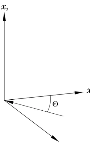
Figure 2. Standard meteorological convention of depicting the
mean wind direction.
2.1 Formulation of the objective function
Equation (4) is valid for the mean wind direction aligned in thex1direction. Following standard meteorological conven-tions, let us consider the mean wind direction to be at an angle 2 with respect to the north, i.e.x2 axis as shown in Fig. 2. At first we derive an objective function for the wind aligned with thex1axis, and then extend the derivation to the coordinate system aligned with the mean wind direction. 2.1.1 Mean wind aligned with thex1axis
If we consider thatδ6is the random error on6, andδSis the random error onS, then Eq. (5) can be written as, M(6+δ6)=S+δS,
6+δ6=M−1(S+δS). (6)
We can thus write,
δ6=M−1δS. (7)
If we consider the sum of the error variances hδ6Tδ6i, where T denotes matrix transpose, then the objective is to minimize the sum of the error variances of the components of6. Taking the transpose and multiplying by Eq. (7) we get, δ6·δ6=δ6Tδ6=(M−1δS)T(M−1δS)
=δST(M−1TM−1)δS (8)
The task now is to simplify Eq. (8) such that it can be rep-resented as a function ofθandφonly. If we assume that the
random errors in the variances of the radial velocities are in-dependent of each other, and that the error variance for each radial velocity variance ishs2i, we get,
δ6Tδ6
2 s
=Tr(M
−1M−1T), (9)
where Tr is the trace of a matrix. The objective function is to minimize Eq. (9).
2.1.2 Coordinate system aligned with the mean wind direction
In order to align the coordinate system with the mean wind direction, we need to apply coordinate transformations on any tensors that are defined in the original coordinate sys-tem. The vectorv rotated in the mean wind direction has to be multiplied by a transformation matrix T given as,
T=
−sin2 −cos2 0 cos2 −sin2 0
0 0 1
. (10)
In the coordinate system aligned with the mean wind di-rection, we then get in matrix form,
Rr=TRTT, (11)
where Rris the Reynolds stress tensor in a coordinate system aligned with the mean wind direction. If we denote6ras the vector of the components of Rr, then we can write,
6r=
sin22 cos22 0 sin 22 0 0 cos22 sin22 0 −sin 22 0 0
0 0 1 0 0 0
−12sin 22 1
2sin 22 0 −cos 22 0 0
0 0 0 0 −sin2 −cos2
0 0 0 0 cos2 −sin2
| {z }
N
6. (12)
Using Eqs. (6) and (7), we can write,
δ6r=NM−1δS (13)
Following the same procedure as in Sect. 2.1.1, we get
δ6rTδ6r
2 s
=Tr(NM
−1(NM−1)T). (14)
Equation (14) states that the error variance is dependent on the mean wind direction. In order to make it independent of the mean wind direction, we assume a uniform distribution of the mean wind direction, and estimate the averaged ratio of the error variance. Thus the directionally averaged ratio is,
δ6rTδ6r
2 s
2
= 1
2π 2π
Z
0
Tr(NM−1(NM−1)T)d2
= 1
2π 2π
Z
0
Tr(NM−1M−1TNT)d2,
we get, δ6T rδ6r 2 s 2 = 1 2π 2π Z 0
Tr(NTNM−1M−1T)d2 (15)
We can also switch the order between integration and ma-trix trace, i.e. either we can estimate the trace first and then the integration or vice-versa. Thus,
δ6rTδ6r
2 s 2 =Tr 1 2π 2π Z 0
NTNd2
M
−1M−1T
. (16)
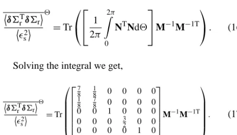
Solving the integral we get,
δ6T
rδ6r 2 s 2 =Tr 7
8 18 0 0 0 0
1 8
7
8 0 0 0 0
0 0 1 0 0 0
0 0 0 32 0 0
0 0 0 0 1 0
0 0 0 0 0 1
M−1M−1T . (17)
The objective is to minimize Eq. (17), subject to the con-straints that θ varies between 0 and 360◦andφ varies be-tween 0 and 45◦. The limit of 45◦ for φ is arbitrary, and is based on the considerations of statistical homogeneity in a horizontal plane. Depending on the type of the terrain the range ofφcould thus be increased or decreased, i.e. if a ter-rain is horizontally homogeneous over a very large extent, thenφcould be greater than 45◦and vice-versa.
2.2 Optimizing the objective function
Equation (17) represents a non-linear optimization problem with 12 unknown variables, i.e. six unknowns are zenith an-glesφ, and the remaining six are the azimuth anglesθ. Ow-ing to the complexity of the optimization problem, an analyt-ical solution of Eq. (17) is not possible. We thus use numer-ical methods, where either gradient or direct search methods could be used (Rao, 2009). For gradient methods, it is essen-tial that the objective function is differentiable. However we assume that Eq. (17) is a discontinuous function, and hence, we do not use gradient methods. Thus we optimize Eq. (17) using direct search methods only. The main advantage of us-ing direct search methods is that they can be used for discon-tinuous and non-differentiable functions. The main limitation of such methods is that the found optimum may only be a lo-cal optimum.
Different algorithms such as simplex (Nelder and Mead, 1965), simulated annealing (Ingber, 1993) and random search (Rao, 2009) are tested, which result in the optimum angles as given in Table 1, which shows that the optimum configuration consists of five beams equally spaced on the base of a scanning cone and one vertical beam.
Table 1. Optimum six-beam configuration.
Beam no. 1 2 3 4 5 6
θ◦ 0 72 144 216 288 288 φ◦ 45 45 45 45 45 0
3 Description of the measurements
The six-beam measurements were carried out using the newly developed 1543 nm pulsed coherent Doppler scanning lidar “long-range WindScanner” (henceforth referred to as WindScanner) at the DTU Wind Energy Department in Den-mark. The WindScanner is based on the pulsed lidar Wind-cube 200 from Leosphere and a dual-axis mirror based steer-able scanner head designed by DTU Wind Energy and IPU. The WindScanner is intended for radial velocity measure-ments from the range of distances between 50 and 6000 m. The current maximum measurement rate is 10 Hz. The max-imum number of simultaneous radial velocities acquired at any rate along each line-of-sight is 500. The WindScanner can emit either 400 or 200 ns laser pulses, which are streamed with two corresponding pulse repetition frequencies of 10 and 20 kHz respectively. The energy content of 400 ns laser pulses is 100 µJ, while the energy content of the 200 ns laser pulses is half of this value. The scanner head has two rota-tional degrees of freedom and can rotate around the azimuth and elevation axes, thus it directs the laser pulses into the at-mosphere at any combination of azimuth and elevation. The maximum scanner head rotation speed is 50◦s−1, while the maximum acceleration is 100◦s−2. The scanner head can ro-tate around both axes from 0 to 360◦, and the rotation can be endless. The pointing accuracy of the WindScanner is 0.05◦. The WindScanner is operated via a remote “master computer” through a UDP/IP and TCP/IP network using the remote sensing communication protocol (RSComPro) (Vasil-jevic, 2014).
5000 5500 6000 6500 7000 5000
5500 6000 6500
UTM 32 Easting-441000 m
UTM
32Northing
-6250000
m
WindScanner
Turbines
89 m
116 m
North Sea
fjord Høvsøre
0 5 10 15
Height above sea [m]
Figure 3. Location of the Høvsøre test centre in Denmark (inset)
and details of the site, where the location of the WindScanner and the met masts are shown.
of the random errors in turbulence measurements (Lenschow et al., 1994). The site is about 2 km from the west coast of Denmark. The eastern sector is characterized by flat homo-geneous terrain, and to the south is a lagoon. The Wind-Scanner is placed at the UTM zone 32 V 447 188 m E and 6 256 189 m N (WGS84 datum) which is about 41 m away from the met mast in the west direction. Since the wind tur-bines are to the east of the WindScanner and the met mast, only the measurements from the western sector (225–315◦) are used. Owing to the sudden change in the surface rough-ness from sea to land in the western sector, we expect the turbulence structure to be influenced by the development of the internal boundary layer, particularly under different at-mospheric stabilities. However we do not expect a significant influence on the flow homogeneity in the horizontal direction around the scanning circle, which is one of the key assump-tions of the six-beam method.
The duration of the full cycle of the six-beam measure-ments from the WindScanner was about 15 s. The period of measurement was between 1 and 28 July 2013, where 764 30 min periods were measured. After filtering for data avail-ability within each 30 min period, where only those periods were chosen with 95 % data, the number of 30 min periods reduced to 625. Finally filtering for wind directions to avoid wakes from the wind turbines and the met mast rendered 401 30 min periods. The available 30 min ensembles are further classified into different atmospheric stabilities, characterized by Monin–Obukhov lengthLMObased on the intervals given in Table 2 (Sathe et al., 2011a).
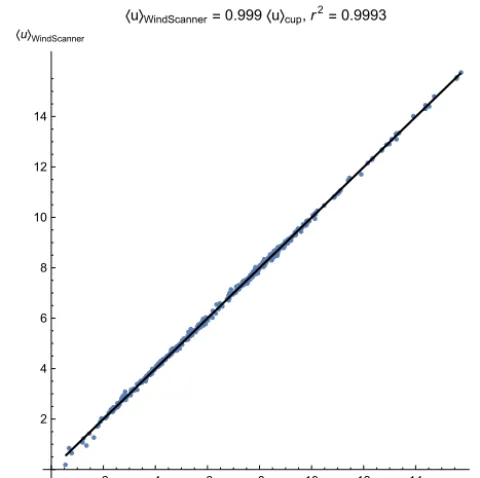
2 4 6 8 10 12 14 〈u〉cup
2 4 6 8 10 12 14 〈u〉WindScanner
〈u〉WindScanner=0.999〈u〉cup,r2=0.9993
Figure 4. Comparison of the 30 min mean wind speed between the
WindScanner and a cup anemometer using two methods.
Table 2. Classification of atmospheric stability according to
Monin–Obukhov length intervals.
unstable (u) −500≤LMO≤ −50 m
neutral (n) |LMO|≥500 m
stable (s) 10≤LMO≤500 m
LMO is estimated using the eddy covariance method (Kaimal and Finnigan, 1994) from the high frequency (20 Hz) measurements of a sonic anemometer at 80 m, that is mounted on a 116 m tall met mast (UTM zone 32 V 447 647 m E and 6 255 435 m N WGS84 datum) in the south-east direction (see Fig. 3). Mathematically,LMOis given as, LMO= −
u∗3θv
κgw0θ0 v
, (18)
whereu∗is the friction velocity,κ=0.4 is the von Kármán constant,gis the acceleration due to gravity, θv is the vir-tual potential temperature,. . .denotes time average, andw0θ0 v (covariance ofwandθv) is the virtual kinematic heat flux.u∗ is estimated as,
u∗= 4
q
u0w02+v0w02, (19)
0.5 1.0 1.5 2.0 〈u' 2〉
Cup 0.5
1.0 1.5 2.0 〈u'2〉WindScanner
〈u'2〉WindScanner=0.85〈u'2〉Cup,r2=0.824
(a)hu02isix-beam
0.5 1.0 1.5 2.0 〈u'
2〉 Cup 0.5
1.0 1.5 2.0 〈u'2〉
WindScanner 〈u'2〉
WindScanner=0.66〈u'2〉Cup,r2=0.795
(b)hu02iVAD
0.25 0.50 0.75 1.00 1.25 1.50 1.75 〈v'
2〉 Cup 0.25
0.50 0.75 1.00 1.25 1.50 1.75 〈v'2
〉WindScanner 〈v'2
〉WindScanner=0.87〈v'2
〉Cup,r2=0.802
(c)hv02isix-beam
0.25 0.50 0.75 1.00 1.25 1.50 1.75 〈v'
2〉 Cup
0.25 0.50 0.75 1.00 1.25 1.50 1.75 〈v'2
〉WindScanner
〈v'2
〉WindScanner=0.84〈v'2
〉Cup,r2=0.843
(d)hv02iVAD
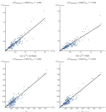
Fig. 5: Comparison of the the turbulence statistics under unstable conditions between the
WindScan-ner and the cup anemometer using two methods
to fit the cup anemometer measurements. The scatter using both methods is comparable to each
other, but there is a slightly more scatter using the six-beam method forhv02 i. 205
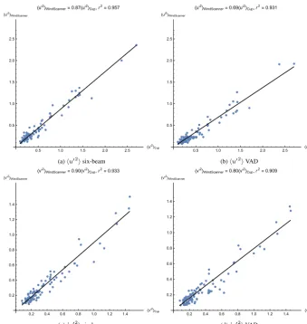
Fig. 6 shows the same as Fig. 5 but under neutral conditions. As for the unstable conditions, the
six-beam method measures more turbulence, about 18%forhu02
iand 10%forhv02
ithan the VAD
method. The scatter using both methods is comparable to each other, with the six-beam method
giving a slightly reduced scatter than the VAD method.
Fig. 7 shows the same as Fig. 5 but under stable conditions. As for the unstable conditions, the 210
six-beam method measures more turbulence, about 19%forhu02
iand 4%forhv02
ithan the VAD
method. The scatter using both methods is comparable to each other, but there is a slightly more
13
Figure 5. Comparison of the turbulence statistics under unstable conditions between the WindScanner and the cup anemometer using two
methods.
and precise (coefficient of determination, r2≈0.9993) in measuring the mean wind speeds. For one 30 min period, the mean radial velocities measured by each of the six beams on the base of the scanning cone were fitted to Eq. (2) in a least squares sense to obtain the 30 min mean wind speed. This procedure was repeated for all 30 min periods. It is to be noted that the mean wind speed obtained using both methods (six-beam and VAD) is identical, since averaging the radial velocity for each beam, and then making a linear fit to ob-tain the u,v, anwcomponents commute. Such an exercise provided enough confidence to proceed with deducing the turbulence measurements from the WindScanner using both methods.
4 Turbulence measurements
Two methods are used to deduce the turbulence statistics from the WindScanner measurements:
1. Six-beam method – for each 30 min period the measured Svector is used in combination with Eq. (5) to deduce
the6vector. Finally the6vector is rotated in the mean wind direction for the respective 30 min period.
0.5 1.0 1.5 2.0 2.5 〈u'
2 〉Cup
0.5 1.0 1.5 2.0 2.5
〈u'2〉 WindScanner
〈u'2〉
WindScanner=0.87〈u'2〉Cup,r2=0.957
(a)hu02isix-beam
0.5 1.0 1.5 2.0 2.5 〈u'
2
〉Cup
0.5 1.0 1.5 2.0 2.5 〈u'2〉
WindScanner
〈u'2〉
WindScanner=0.69〈u'2〉Cup,r2=0.931
(b)hu02iVAD
0.2 0.4 0.6 0.8 1.0 1.2 1.4 〈v'
2〉 Cup
0.2 0.4 0.6 0.8 1.0 1.2 1.4
〈v'2 〉WindScanner
〈v'2
〉WindScanner=0.90〈v'2
〉Cup,r2=0.933
(c)hv02 isix-beam
0.2 0.4 0.6 0.8 1.0 1.2 1.4 〈v' 2〉
Cup 0.2
0.4 0.6 0.8 1.0 1.2 1.4
〈v'2
〉WindScanner
〈v'2
〉WindScanner=0.80〈v'2
〉Cup,r2=0.909
(d)hv02
iVAD
Fig. 6: Comparison of the the turbulence statistics under neutral conditions between the
WindScan-ner and the cup anemometer using two methods
scatter using the six-beam method forhu02 i.
Thus under all stabilities the six-beam method is closer to the turbulence measurements carried
out using the reference cup anemometer. There is however some probe volume averaging using both 215
methods, but is significantly larger for the VAD method.
5 Discussion
From Figs. 5–7 it is clear that using both methods the WindScanner measures more turbulence under
stable conditions than under unstable and neutral conditions. This may be contrary to our intuitive
14
Figure 6. Comparison of the turbulence statistics under neutral conditions between the WindScanner and the cup anemometer using two
methods.
Figure 6 shows the same as Fig. 5 but under neutral con-ditions. As for the unstable conditions, the six-beam method measures more turbulence, about 18 % forhu02iand 10 % for
hv02ithan the VAD method. The scatter using both methods is comparable to each other, with the six-beam method giving a slightly reduced scatter than the VAD method.
Figure 7 shows the same as Fig. 5 but under stable con-ditions. As for the unstable conditions, the six-beam method measures more turbulence, about 19 % forhu02iand 4 % for
hv02ithan the VAD method. The scatter using both methods is comparable to each other, but there is slightly more scatter using the six-beam method forhu02i.
Thus under all stabilities the six-beam method is closer to the turbulence measurements carried out using the reference cup anemometer. There is however some probe volume av-eraging using both methods, but this is significantly larger for the VAD method. The probe volume averaging can be observed clearly by comparing the radial velocity spectra, which can be observed in Fig. 6 in Mann et al. (2009), and Fig. 4 in Sjöholm et al. (2009).
5 Discussion
0.1 0.2 0.3 0.4 0.5 0.6 〈u'
2 〉Cup
0.1 0.2 0.3 0.4 0.5 0.6
〈u'2〉 WindScanner
〈u'2〉
WindScanner=1.01〈u'2〉Cup,r2=0.730
(a)hu02isix-beam
0.1 0.2 0.3 0.4 0.5 0.6 〈u'
2
〉Cup
0.1 0.2 0.3 0.4 0.5 0.6 〈u'2〉
WindScanner
〈u'2〉
WindScanner=0.82〈u'2〉Cup,r2=0.793
(b)hu02iVAD
0.2 0.4 0.6 0.8 〈v'
2〉 Cup
0.2 0.4 0.6 0.8
〈v'2
〉WindScanner
〈v'2
〉WindScanner=0.91〈v'2
〉Cup,r2=0.829
(c)hv02 isix-beam
0.2 0.4 0.6 0.8 〈v'
2〉 Cup
0.2 0.4 0.6 0.8
〈v'2
〉WindScanner
〈v'2
〉WindScanner=0.87〈v'2
〉Cup,r2=0.804
(d)hv02
iVAD
Fig. 7: Comparison of the the turbulence statistics under stable conditions between the WindScanner
and the cup anemometer using two methods
understanding, because usually the turbulence scales are much larger under unstable conditions than 220
under stable conditions (Sathe et al., 2013). These results are also contrary to what has been observed
by Sathe et al. (2011b) at the same site. However, it is to be noted that Sathe et al. (2011b) used
the lidar measurements when the wind was blowing from the eastern direction, whereas in this work
we use the measurements when the wind is blowing from the western direction. As described in
section 4, in the western sector there is a sudden change of roughness due to the transition from 225
sea to land. As a consequence there is a development of the internal boundary layer (IBL). Also
the growth of the IBL depends on atmospheric stability, where under unstable conditions the growth
will be faster than under stable conditions. Panofsky and Dutton (1984) state that the growth of the
15
Figure 7. Comparison of the turbulence statistics under stable conditions between the WindScanner and the cup anemometer using two
methods.
height of the boundary layer is proportional to the drag coefficientu∗/hui. And it is well known that
the drag coefficient is larger for unstable stratification. Consequently the turbulence scales within 230
the IBL will be smaller as compared to those outside of it. It is then interesting to check whether
the WindScanner measures more within the IBL under unstable conditions as compared to the stable
conditions.
10-3 10-2 10-1 100
10-2
10-1
k1
k1
×
Fuu
(
k1
)
Unstable
Neutral Stable
(a)u-spectra
10-3 10-2 10-1 100
10-2
k1
k1
×
Fvv
(
k1
)
Unstable
Neutral Stable
(b)v-spectra
Fig. 8: Comparison of theu- andv-spectra derived from high-frequency cup anemometer
measure-ments under different stability conditions
Fig. 8 shows theu- andv-spectra derived from high-frequency cup anemometer measurements
under different stability conditions. If we define the characteristic length scaleLas the length scale 235
corresponding to the maximum spectral energy, it is then clear that the peak of thev-spectra is
shifted to the right for unstable conditions as compared to the stable conditions. It is not that clear
for theu-spectra, however the shift of scales to larger wavenumbers under unstable conditions can
still be observed. ThusLappears smaller under unstable conditions than under stable conditions
for the measurements from the western sector used in this work. There is thus more probe volume 240
averaging under unstable conditions than under stable conditions. Hence the WindScanner attenuates
the turbulence measurements lesser under unstable conditions than under stable conditions.
Another interesting observation is that using the VAD method the WindScanner does not measure
more turbulence than the reference cup anemometer under any stability condition. This does not
agree with that observed by Sathe et al. (2011b), even though the same basic pulsed commercial 245
lidar technology was also used in that work. It is likely due to the fact that in Sathe et al. (2011b)
only four beams were used as opposed to six beams, andαwas 60◦compared to 45◦used in this
work. Therefore the turbulence statistics are not directly comparable with those obtained in Sathe
et al. (2011b) even though the same basic commercial lidar was used. Due to the application of the
least squares technique on thevrmeasurements in this work, there is significant volume averaging 250
around the scanning circle, which is also observed in Sathe et al. (2011b) for a continuous-wave
lidar.
Figure 8. Comparison of theu- andv-spectra derived from high-frequency cup anemometer measurements under different stability conditions
to the drag coefficientu∗/hui. And it is well known that the drag coefficient is larger for unstable stratification. Conse-quently the turbulence scales within the IBL will be smaller as compared to those outside of it. It is then interesting to check whether the WindScanner measures more within the IBL under unstable conditions as compared to the stable con-ditions.
Figure 8 shows theu andv spectra derived from high-frequency cup anemometer measurements under different stability conditions. If we define the characteristic length scaleLas the length scale corresponding to the maximum spectral energy, it is then clear that the peak of thev spec-tra is shifted to the right for unstable conditions as compared to the stable conditions. It is not that clear for theu spec-tra, however the shift of scales to larger wavenumbers
der unstable conditions can still be observed. ThusLappears smaller under unstable conditions than under stable condi-tions for the measurements from the western sector used in this work. There is thus more probe volume averaging under unstable conditions than under stable conditions. Hence the WindScanner attenuates the turbulence measurements more under unstable conditions than under stable conditions.
Another interesting observation is that using the VAD method the WindScanner does not measure more turbulence than the reference cup anemometer under any stability con-dition. This, too, does not agree with that observed by Sathe et al. (2011b), even though the same basic pulsed commer-cial lidar technology was also used in that work. It is likely due to the fact that in Sathe et al. (2011b) only four beams were used as opposed to six beams, and α was 60◦ com-pared to 45◦ used in this work. Therefore the turbulence statistics are not directly comparable with those obtained in Sathe et al. (2011b) even though the same basic commercial lidar was used. Due to the application of the least squares technique on thevrmeasurements in this work, there is sig-nificant volume averaging around the scanning circle, which is also observed in Sathe et al. (2011b) for a continuous-wave lidar.
6 Conclusions
An alternative so-called six-beam method is proposed in place of the standard VAD method to measure atmospheric turbulence using a ground-based wind lidar. The major difference between the two methods is that the six-beam method uses the measurement of the radial velocity vari-ances, whereas the VAD method uses the high frequency measurement of the radial velocity transformed into Carte-sian coordinates to deduce turbulence statistics. The scan-ning configuration of the six-beam method is optimized to minimize the sum of the random errors in the measurement of the components of the R matrix. In comparison to the ref-erence cup anemometer the six-beam method measures be-tween 85 and 101 % of the reference turbulence, whereas the VAD method measures between 66 and 87 % depending on atmospheric stability. The six-beam method thus overcomes partly the problem of significant probe volume averaging that is otherwise observed by the VAD method.
Furthermore two interesting observations have been made in this study. One is that, using both methods the WindScan-ner measures more turbulence under stable conditions than under unstable conditions, mainly due to the influence of the internal boundary layer (see Sect. 5). The other is that de-spite using the same underlying pulsed lidar technology as in Sathe et al. (2011b), the VAD method never measures more turbulence than the reference instrument as was observed in Sathe et al. (2011b) (see Sect. 5 for some explanation). It emphasizes the point that the VAD method is highly
sensi-tive to the turbulence structure in the atmosphere, and one must avoid using it to measure atmospheric turbulence.
Future studies must certainly focus on tackling the probe volume averaging effect, which will further strengthen the arguments of using the six-beam method. Smalikho et al. (2005) have provided us with such a framework for pulsed lidars, whereas Mann et al. (2010) have demonstrated it for a continuous-wave lidar.
Acknowledgements. This work is carried out as a part of a research project funded by the Danish Ministry of Science, Innovation and Higher Education – Technology and Production, grant no. 0602-02486B. The resources provided by the Center for Computational Wind Turbine Aerodynamics and Atmospheric Turbulence funded by the Danish Council for Strategic Research grant no. 09-067216 are also acknowledged. We also thank Erik Juul from DTU Wind Energy department for helping with some sketches.
Edited by: W. Ward
References
Banakh, V. A. and Smalikho, I. N.: Determination of the turbulent energy dissipation rate from lidar sensing data, Atmos. Ocean. Opt., 10, 295–302, 1997a.
Banakh, V. A. and Smalikho, I. N.: Estimation of the turbulence en-ergy dissipation rate from the pulsed Doppler lidar data, Atmos. Ocean. Opt., 10, 957–965, 1997b.
Banakh, V. A. and Werner, C.: Computer simulation of co-herent Doppler lidar measurement of wind velocity and re-trieval of turbulent wind statistics, Opt. Eng., 44, 071205, doi:10.1117/1.1955167, 2005.
Banakh, V. A., Smalikho, I. N., Köpp, F., and Werner, C.: Repre-sentativeness of wind measurements with a CW Doppler lidar in the atmospheric boundary layer, Appl. Opt., 34, 2055–2067, doi:10.1364/AO.34.002055, 1995a.
Banakh, V. A., Werner, C., Kerkis, N. N., Köpp, F., and Smalikho, I. N.: Turbulence measurements with a CW Doppler lidar in the atmospheric boundary layer, Atmos. Ocean. Opt., 8, 955–959, 1995b.
Banakh, V. A., Werner, C., Köpp, F., and Smalikho, I. N.: Measure-ment of turbulent energy dissipation rate with a scanning Doppler lidar, Atmos. Ocean. Opt., 9, 849–853, 1996.
Banakh, V. A., Smalikho, I. N., Köpp, F., and Werner, C.: Measurements of turbulent energy dissipation rate with a CW Doppler lidar in the atmospheric boundary layer, J. Atmos. Ocean. Technol., 16, 1044–1061, doi:10.1175/1520-0426(1999)016<1044:MOTEDR>2.0.CO;2, 1999.
Banakh, V. A., Smalikho, I. N., Pichugina, Y. L., and Brewer, W. A.: Representativeness of measurements of the dissipation rate of turbulence energy by scanning Doppler lidar, Atmos. Ocean. Opt., 23, 48–54, doi:10.1134/S1024856010010100, 2010. Branlard, E., Pedersen, A. T., Mann, J., Angelou, N., Fischer, A.,
Browning, K. A. and Wexler, R.: The determination of kinematic properties of a wind field using a Doppler radar, J. Appl. Meteorol., 7, 105–113, doi:10.1175/1520-0450(1968)007<0105:TDOKPO>2.0.CO;2, 1968.
Clifton, A., Elliott, D., and Courtney, M.: Ground-Based vertically profiling remote sensing for wind resource assessment, Tech. Rep. 15, Internation Energy Agency, 2013.
Eberhard, W. L., Cupp, R. E., and Healy, K. R.: Doppler li-dar measurements of profiles of turbulence and momentum flux, J. Atmos. Ocean. Technol., 6, 809–819, doi:10.1175/1520-0426(1989)006<0809:DLMOPO>2.0.CO;2, 1989.
Frehlich, R.: Coherent Doppler lidar signal covariance including wind shear and wind turbulence, Appl. Opt., 33, 6472–6481, doi:10.1364/AO.33.006472, 1994.
Frehlich, R.: Effects of wind turbulence on coherent Doppler lidar performance, J. Atmos. Ocean. Technol., 14, 54–75, doi:10.1175/1520-0426(1997)014<0054:EOWTOC>2.0.CO;2, 1997.
Frehlich, R. and Cornman, L.: Estimating spatial velocity statistics with coherent Doppler lidar, J. Atmos. Ocean. Techno., 19, 355– 366, doi:10.1175/1520-0426-19.3.355, 2002.
Frehlich, R. and Kelley, N.: Measurements of wind and turbulence profiles with scanning Doppler lidar for wind energy applica-tions, IEEE J. Selected Topics Appl. Earth Obs. Remote Sens., 1, 42–47, doi:10.1109/JSTARS.2008.2001758, 2008.
Frehlich, R., Hannon, S. M., and Henderson, S. W.: Performance of a 2-µm coherent Doppler lidar for wind measurements, J. Atmos. Ocean. Technol., 11, 1517–1528, doi:10.1175/1520-0426(1994)011<1517:POACDL>2.0.CO;2, 1994.
Frehlich, R., Hannon, S. M., and Henderson, S. W.: Coherent Doppler lidar measurements of wind field statistics, Bound.-Lay. Meteorol., 86, 233–256, doi:10.1023/A:1000676021745, 1998. Frehlich, R., Meillier, Y., Jensen, M. L., Balsley, B., and
Shar-man, R.: Measurements of boundary layer profiles in ur-ban environment, J. Appl. Meteorol. Climatol., 45, 821–837, doi:10.1175/JAM2368.1, 2006.
Frehlich, R., Meillier, Y., and Jensen, M. L.: Measure-ments of boundary layer profiles with in situ sensors and Doppler lidar, J. Atmos. Ocean. Technol., 25, 1328–1340, doi:10.1175/2007JTECHA963.1, 2008.
Gal-Chen, T., Xu, M., and Eberhard, W. L.: Estimation of atmo-spheric boundary layer fluxes and other turbulence parameters from Doppler lidar data, J. Geophys. Res., 97, 18409–18423, doi:10.1029/91JD03174, 1992.
Ingber, L.: Simulated Annealing: Practice versus Theory, Math. Comput. Model., 18, 29–57, 1993.
Kaimal, J. C. and Finnigan, J. J.: Atmospheric Boundary Layer Flows – Their Structure and Measurement, chap. Acquisition and processing of atmospheric boundary layer data, 254–281, 7, Ox-ford University Press, New York, 1994.
Kindler, D., Oldroyd, A., Macaskill, A., and Finch, D.: An eight month test campaign of the QinetiQ ZephIR system: Prelim-inary results, Meteorol. Z., 16, 479–489, doi:10.1127/0941-2948/2007/0226, 2007.
Kropfli, R. A.: Single Doppler radar measurement of tur-bulence profiles in the convective boundary layer, J. Atmos. Ocean. Technol., 3, 305–314, doi:10.1175/1520-0426(1986)003<0305:SDRMOT>2.0.CO;2, 1986.
Lenschow, D. H., Mann, J., and Kristensen, L.: How long is long enough when measuring fluxes and other turbulence statistics?, J. Atmos. Ocean. Technol., 11, 661–673, doi:10.1175/1520-0426(1994)011<0661:HLILEW>2.0.CO;2, 1994.
Lhermitte, R. M.: Note on wind variability with Doppler radar, J. Atmos. Sci., 19, 343–346, doi:10.1175/1520-0469(1962)019<0343:NOWVWD>2.0.CO;2, 1962.
Lhermitte, R. M.: Note on the observation of small-scale atmo-spheric turbulence by Doppler radar techniques, Radio Sci., 4, 1241–1246, doi:10.1029/RS004i012p01241, 1969.
Mann, J., Cariou, J., Courtney, M., Parmentier, R., Mikkelsen, T., Wagner, R., Lindelow, P., Sjöholm, M., and Enevoldsen, K.: Comparison of 3D turbulence measurements using three staring wind lidars and a sonic anemometer, Meteorol. Z., 18, 135–140, doi:10.1127/0941-2948/2009/0370, 2009.
Mann, J., Peña, A., Bingöl, F., Wagner, R., and Courtney, M. S.: Lidar scanning of momentum flux in and above the surface layer, J. Atmos. Ocean. Technol., 27, 792–806, doi:10.1175/2010JTECHA1389.1, 2010.
Nelder, J. A. and Mead, R.: A Simplex Method for Function Mini-mization, Computer J., 7, 308–313, 1965.
Panofsky, H. A. and Dutton, J. A.: Atmospheric Turbulence, John Wiley & Sons, New York, 1984.
Peña, A., Hasager, C. B., Gryning, S.-E., Courtney, M., Antoniou, I., and Mikkelsen, T.: Offshore Wind Profiling Using Light De-tection and Ranging Measurements, Wind Energy, 12, 105–124, doi:10.1002/we.283, 2009.
Rao, S.: Engineering Optimization: Theory and Practice, John Wi-ley and Sons Inc., Hoboken, New Jersey, 4th Edn., 2009. Sathe, A. and Mann, J.: Measurement of turbulence spectra using
scanning pulsed wind lidars, J. Geophys. Res., 117, D01201, doi:10.1029/2011JD016786, 2012.
Sathe, A. and Mann, J.: A review of turbulence measurements using ground-based wind lidars, Atmos. Meas. Tech., 6, 3147–3167, doi:10.5194/amt-6-3147-2013, 2013.
Sathe, A., Gryning, S.-E., and Peña, A.: Comparison of the atmo-spheric stability and wind profiles at two wind farm sites over a long marine fetch in the North Sea, Wind Energy, 14, 767–780, doi:10.1002/we.456, 2011a.
Sathe, A., Mann, J., Gottschall, J., and Courtney, M. S.: Can wind lidars measure turbulence?, J. Atmos. Ocean. Technol., 28, 853– 868, doi:10.1175/JTECH-D-10-05004.1, 2011b.
Sathe, A., Mann, J., Barlas, T., Bierbooms, W. A. A. M., and van Bussel, G. J. W.: Influence of atmospheric stability on wind tur-bine loads, Wind Energy, 16, 1013–1032, doi:10.1002/we.1528, 2013.
Sjöholm, M., Mikkelsen, T., Mann, J., Enevoldsen, K., and Court-ney, M.: Spatial averaging-effects on turbulence measured by a continuous-wave coherent lidar, Meteorol. Z., 18, 281–287, doi:10.1127/0941-2948/2009/0379, 2009.
Smalikho, I., Kopp, F., and Rahm, S.: Measurement of atmospheric turbulence by 2-µm Doppler lidar, J. Atmos. Ocean. Technol., 22, 1733–1747, doi:10.1175/JTECH1815.1, 2005.
Smalikho, I. N.: On measurement of dissipation rate of the turbulent energy with a CW Doppler lidar, Atmos. Ocean. Opt., 8, 788– 793, 1995.
the Danish Wind Test Site in Høvsøre, Wind Energy, 9, 87–93, doi:10.1002/we.193, 2006.
Vasiljevic, N.: A time-space synchronization of coherent Doppler scanning lidars for 3D measurements of wind fields, Ph.D. Thesis PhD-0027 (EN), Technical University of Denmark, 2014.
Wagner, R., Courtney, M., Gottschall, J., and Lindelöw-Marsden, P.: Accounting for the speed shear in wind turbine power performance measurement, Wind Energy, 14, 993–1004, doi:10.1002/we.509, 2011.