www.earth-syst-dynam.net/5/1/2014/ doi:10.5194/esd-5-1-2014
© Author(s) 2014. CC Attribution 3.0 License.
Earth System
Dynamics
An interaction network perspective on the relation between patterns
of sea surface temperature variability and global mean surface
temperature
A. Tantet and H. A. Dijkstra
Institute for Marine and Atmospheric research Utrecht, Utrecht University, Utrecht, the Netherlands Correspondence to: A. Tantet ([email protected])
Received: 25 July 2013 – Published in Earth Syst. Dynam. Discuss.: 12 August 2013 Revised: 25 November 2013 – Accepted: 26 November 2013 – Published: 3 January 2014
Abstract. On interannual- to multidecadal timescales vari-ability in sea surface temperature appears to be organized in large-scale spatiotemporal patterns. In this paper, we in-vestigate these patterns by studying the community structure of interaction networks constructed from sea surface tem-perature observations. Much of the community structure can be interpreted using known dominant patterns of variability, such as the El Niño/Southern Oscillation and the Atlantic Multidecadal Oscillation. The community detection method allows us to bypass some shortcomings of Empirical Orthog-onal Function analysis or composite analysis and can pro-vide additional information with respect to these classical analysis tools. In addition, the study of the relationship be-tween the communities and indices of global surface temper-ature shows that, while El Niño–Southern Oscillation is most dominant on interannual timescales, the Indian West Pacific and North Atlantic may also play a key role on decadal timescales. Finally, we show that the comparison of the com-munity structure from simulations and observations can help detect model biases.
1 Introduction
An important issue in climate research is to understand the behavior of the global mean surface temperature (GMST) over the last century (Sutton et al., 2007). Both internal variability and changes in radiative forcing, in particular by anthropogenic emissions of greenhouse gases (GHG), con-tribute to changes in GMST. The impact of GHG forcing has been extensively studied, being highly relevant to
cli-mate sensitivity and hence for projections on future changes of the GMST. The important role of internal variability of ocean heat storage on GMST has been highlighted in the re-cent study by Balmaseda et al. (2013).
On interannual- to multidecadal timescales, climate vari-ability appears to be organized into large-scale patterns with the El Niño/Southern Oscillation (ENSO) and the Atlantic Multidecadal Oscillation (AMO) as prominent examples. These phenomena are characterized by well-defined spa-tiotemporal patterns in sea surface temperature (SST). The ENSO variability in the equatorial Pacific is the dominant pattern of variability on interannual timescales (Mcphaden et al., 1998; Wang et al., 2004). ENSO influences the cli-mate of many regions over the globe (Alexander and Bladé, 2002; Deser et al., 2010) and the El Niño 1997–1998 event was estimated to have caused a GMST increase of about 0.6◦C (Trenberth, 1997). The AMO is the dominant pattern of SST variability in the North Atlantic on decadal- to mul-tidecadal timescales (Enfield, 2001). The AMO is thought to be strongly related to variations in the Atlantic Meridional Overturning Circulation (Srokosz et al., 2012), which affect the oceanic meridional heat transport. Sutton and Hodson (2005) show that the AMO has an influence on European Summer temperatures and relations of the AMO with US rainfall were suggested in Enfield (2001). Recently, it was suggested that the variability of global land surface tempera-tures (GLST) is strongly connected to the AMO (Canty et al., 2013), with a correlation coefficient of 0.65±0.04 (Muller et al., 2013).
first mode, are usually difficult to relate to the patterns of variability as known from regional EOF analyses (Monahan et al., 2009). It is therefore still quite unclear how and how much the different patterns and their interaction contribute to GMST variability.
Here we address the problem on the connection between patterns of SST variability and GMST using complex net-works theory. Although this theory has already been success-fully applied to many different technological and scientific problems (e.g. in computer sciences, neurosciences, social sciences) it has only recently that it been used in climate re-search. So-called interaction networks, where links are based on a correlation measurement between variables at specific locations, have been reconstructed to analyze the connectiv-ity of the climate system (Tsonis and Roebber, 2004; Tso-nis et al., 2010; Donges et al., 2009b, a), teleconnections (Tsonis et al., 2008), the behavior of El Niño (Gozolchi-ani et al., 2008, 2011; Tsonis and Swanson, 2008; Yamasaki et al., 2008), synchronization between different spatiotem-poral patterns (Tsonis et al., 2007; Wyatt et al., 2011) and the connections between the variability in different climate variables (Donges et al., 2011).
One of the many interesting properties of a network is its possible partition into communities or groups of highly connected nodes which are only weakly connected to the rest of the network. Community detection has recently been applied to climate interaction networks of different atmo-spheric variables from observations and simulations by (Tso-nis et al., 2010) where some of the known patterns of at-mospheric variability, such as the North Atlantic Oscillation, could be identified.
We focus in this study on communities in interaction net-works reconstructed from global SST observations. The data, their preprocessing and the network reconstruction and anal-ysis tools are presented in Sect. 2. In Sect. 3, results on the SST communities in the reconstructed networks are pre-sented and interpreted, and connected to results in the litera-ture based on EOF and composite analysis. Then in Sect. 4, we address the connection between the SST communities and the GMST and also compare the results from observa-tions with those from Earth system model (ESM) simula-tions. In the Sect. 5, the main results are summarized and discussed with a focus on the benefits of the interaction network approach.
trended monthly data. Even though the leading order effect of the annual cycle is removed by producing anomaly val-ues, boreal winter anomalies are still larger than in summer. In order to avoid spurious high values of correlations, Tso-nis and Roebber (2004) and TsoTso-nis et al. (2010) only used the December-January-February months of each year. Since our results were not significantly affected by the selection of the winter months, we decided to use complete years. The detrended monthly anomalies were then low-pass filtered via a Lanczos filter (Duchon, 1979) with a cutoff frequency of 1/13 month−1and order 144.
Because more grid points are located towards the poles on a regular longitude-latitude grid, which could lead to bi-ases in our network measures, the data was linearly inter-polated on a sinusoidal grid in order to conserve the arc length with latitude. In this study, we used a resolution at the equator of 2◦but the results presented below are quali-tatively similar when using grid resolutions ranging from 1◦ to 5◦. Because of the poor sampling of the region south of 50◦S (Deser et al., 2010, Fig. 3), only the grid points lo-cated between 50◦S and 80◦N were kept, resulting in a total
ofN =6280 grid points (land surface points excluded) for
L=142×12=1704 months.
Each ocean grid point is considered as a node in the net-work and we indicate the time series at nodei,i=1, . . . , N
by pi(tk), k=1, . . . , L. Contrary to a network as derived from a power grid or the world-wide web, the links of a cli-mate network are not directly tangible because the observ-ables derive from continuous fields. In an interaction net-work, a link between two nodes is based on a measure of the correlation between the time series of these two nodes. In this study, we used the Pearson correlation coefficient at lag zero, sayRij, between the time series of nodesiandj, defined by
Rij =
PL
k=1pi(tk)pj(tk)
q
(PL
k=1p2i(tk))(
PL
k=1pj2(tk)))
(1)
as the measure defining the links in the network (Tsonis and Roebber, 2004). A pair of nodes is then considered to be con-nected if their correlationRij is over a chosen thresholdτ. The elementsaij of the N×N adjacency matrix A of the undirected and unweighted network are thus given by
aij =2(Rij−τ )−δij, (2)
are based on SST correlations at zero lag, a connection should not be considered instantaneous, since the time se-ries were low-pass filtered for 13 months. However, Foster and Rahmstorf (2011) found that lags ranging from 0 to 7 months are relevant to the study of interannual climate vari-ability. Our results have been tested for lagged correlations in this range. Since no qualitative differences were found and correlations were generally weaker for longer lags, only the results for 0 lag correlation are presented in this study.
We based our choice of the thresholdτ on parametric and non-parametric significance tests. Considering a decorrela-tion time of 13 months (corresponding to the cut-off fre-quency of the filter), we found that all correlations over 0.17 are statistically significant at the 5 % level according to a t-test withL/13=131 degrees of freedom.
In order to better account for the persistence in the time se-ries, a moving block bootstrap (MBB) test was also applied to the time series (Mudelsee, 2010). The bootstrap works with artificially produced resamples of the time series. In an MBB, blocks of lengthLBare randomly picked out of the original
time series to create a set sizeNS of surrogate time series.
Correlations are then calculated between surrogate time se-ries for each pair of nodes. The choice of the block length is a trade-off between conserving the memory of the origi-nal time series and producing maximally independent surro-gate time series. For the data set used in this study, we found that the estimated 5 % significance level was robust for block lengths ranging from 15 to 50 yr. Consequently, we chose a block length ofLB of 20 yr and a sample set sizeNS of 4000 for all our MBB tests. Because a grid of 6280 nodes results in∼2×10⁷pairs, the MBB tests were realized on a coarser grid of 5◦×5◦resulting in 1144 nodes. We found
that in the worst case thep values of the 5 % significance level was 0.39.
Additionally, an approximate test was used, where corre-lations were calculated between pairs of surrogate time se-ries associated with the same node for the 6280 nodes of the 2◦ grid. Thep values found in this case were close to the maximumpvalues found for each grid point of the first test, suggesting that the approximated version of the MBB test is a good alternative for large gridded data sets.
The results of both parametric and non-parametric tests in-dicate that a thresholdτ =0.4 guarantees that a link between a pair of nodes of the HadISST data represents a statistically significant correlation at the 5 % level. In addition, thresh-olds ranging from 0.4 to 0.6 were used to build the network and we found that our results were not qualitatively sensitive to the threshold value over this range, although teleconnec-tions appear weaker as the threshold increases. Subsequently, a threshold of 0.4 will be used and the resulting interaction network built from the HadISST data set will be referred to as the H-SST network.
2.2 Analysis techniques
Extended reviews of commonly used network measures can be found in Costa and Rodrigues (2007) and Barthélemy (2011). We here focus on degree centrality, first neighbours maps and communities. The degree centralitydi of a nodei counts its number of connections with other nodes of the net-work. This measure is directly accessible from the adjacency matrix through
di = N
X
j=1
aij (3)
and allows one to reveal nodes sharing a common variability with other nodes of the network. The edge density ρ of a network
ρ= 1
N (N−1)
N
X
i,j=1
aij (4)
is the total number of links in the network normalized by the maximum number of possible links and is an indicator of the sparseness of the network. First neighbours maps describe the fraction of nodes belonging to a given group any node in the network is connected to. They are defined as
FNi→G=
1
NG
X
nj∈G
aij, (5)
where “G” is the selected group ofNG nodes. A node of a first neighbours map reaches a maximum (minimum) value of 100 % (0 %) if it is connected to all (none) of the nodes of the selected group of nodes.
Much focus has recently been given to the partitioning of networks into communities (Newman and Girvan, 2004). Communities are groups of nodes tightly connected together and weakly connected to the rest of the network. As such, they can be regarded as subsystems which operate relatively independently of the other communities (Arenas et al., 2006). Considerable improvements have been made during the past decade regarding the speed and efficiency of the commu-nity detection algorithms. In Tsonis et al. (2010), the algo-rithm of Newman and Girvan (2004) based on the progres-sive removal of dominant links (in terms of information flow) was applied to determine the community structure of several fields (500 hPa height, sea level pressure and surface tem-perature) derived from the NCEP/NCAR reanalysis (Kistler et al., 2001) and simulations from the Geophysical Fluid Dynamics Laboratory (GFDL) climate model CM2.1 (Del-worth, 2006).
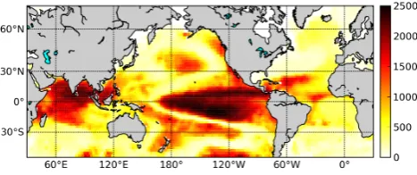
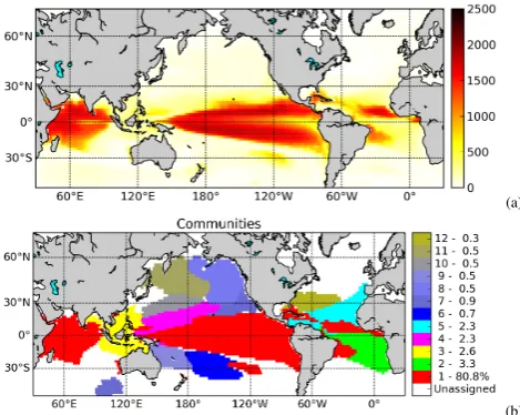
Fig. 1: Degree centrality, as defined by Eq. (3), of the nodes of the H-SST network. A threshold
τ= 0.4was used to construct the network giving an edge densityρ= 0.14.
22
Fig. 1. Degree centrality, as defined by Eq. (3), of the nodes of the
H-SST network. A thresholdτ=0.4 was used to construct the net-work giving an edge densityρ=0.14.
below are generated using the Infomap algorithm by Ros-vall and Bergstrom (2007) which is based on the compression of the paths of random walkers traveling along the network. This algorithm was the most efficient in the LFR benchmark (Lancichinetti and Fortunato, 2009) among the different al-gorithms tested.
3 Spatial structure of SST variability
3.1 Communities in the H-SST network: detection
The map of degree centrality of the H-SST networks (Fig. 1) indicates that nodes located in the tropics tend to have a higher degree centrality than those located in the extra-tropics, in agreement with atmospheric surface temperature analyses in Tsonis and Roebber (2004). The tropical Atlantic shows a rather low degree centrality compared to the Indian and Pacific Oceans except over its northwestern part. The eastern tropical Indian Ocean also shows a low degree trality. Surrounding the tropics, patches of high degree cen-trality are found in the mid-latitude North Pacific, South Pa-cific and along the western coast of the American continent. In order to assess whether the variability in high-degree regions arises from distinct spatial patterns, the community structure of the H-SST network is determined (Fig. 2a). The communities are ordered by the total “PageRank” of their nodes (Brin and Page, 1998). The PageRank corresponds to the fraction of random walkers which would flow through the nodes of a community out of a population of random walkers traveling around the network by the links. In a directed net-work, a large flow of random walkers can arise from the large inward-degree of the nodes they go through but also from the large inward-degree of the nodes pointing to them and so on. However, in our case, the network is undirected so that the flow of random walkers through a node is equal to its degree centrality divided by the edge density. The total PageRank of a community is thus given by
PRi= 1
ρ
X
j∈Ci dj=
1
ρ
X
j∈Ci
X
k
aj k, (6)
Fig. 2: Top panel (a): Infomap communities in the H-SST network. Each color represents one
community and each node is assigned the color of the community it belongs to. The communities
are ordered by decreasing total PageRank of their nodes which is written to the right of the scale.
Bottom panel (b): Infomap communities after filtration of nodes which are connected to a fraction
of their community smaller than twice the density of the network or belong to communities with
nodes smaller than 2% of the network. Nodes in white are unassigned, they do not belong to any
community.
23
Fig. 2. (a) Infomap communities in the H-SST network. Each color
represents one community and each node is assigned the color of the community it belongs to. The communities are ordered by decreas-ing total PageRank of their nodes, which is written to the right of the scale. (b) Infomap communities after filtration of nodes that are connected to a fraction of their community smaller than twice the density of the network or belong to communities with nodes smaller than 2 % of the network. Nodes in white are unassigned, they do not belong to any community.
whereCi is the set of nodes belonging to communityi. Con-sequently, the PageRank of a community is a measure of the co-variability of its nodes.
A common measure of the quality of a partition of a net-work into communities is the modularity of this partition (Newman and Girvan, 2004). For a particular division into
m communities an m×m symmetric matrix e is defined, for which an element eij is the fraction of all connections in the network that link nodes in community i to nodes in communityj. As such,P
ieii gives the fraction of edges in the network that connect nodes in the same community and
fi=Pjeij represents the fraction of all edges in the net-work that connect to nodes in communityi. In a (random) network, for which edges connect nodes independent of the communities they belong to, we would have eij =fifj so thatP
ifi2corresponds to the fraction of all edges that con-nect to the same community in such a randomly wired net-work. In a modular network, the(eii)must be high compar-atively to the(fi2), thus, the modularityMis defined as in Newman and Girvan (2004):
M=
m
X
i=1
(eii−fi2). (7)
Eigenvector algorithms, for the same network. We will now justify our choice of the Infomap algorithm in spite of the lower modularity of its partition of the H-SST network.
The main problematic issue we encountered when apply-ing community detection algorithms to SST networks arises from the spatial heterogeneity of the modularity of these networks. Regions where one spatial pattern of variability dominates (e.g. ENSO) are obviously highly modular. How-ever, regions where the variability is dominated by the ef-fect of atmospheric noise can also be weakly modular, so that the existence of communities in such regions is ques-tionable. It is often more optimal in terms of modularity to associate the nodes of such weakly modular regions to one broad but weakly interconnected community. Such a com-munity cannot be considered as a coherent physical pattern of variability, so that it would be preferable not to associate nodes of weakly modular regions to any community. The community detection algorithms we know must distribute ev-ery node to a community no matter how modular the net-work is. Thus, it would be preferable to distribute nodes of weakly modular regions into several small but densely in-terconnected communities (even if small means one node, in the case of very weakly modular regions). For our net-works, the Infomap algorithm was the most capable one to divide weakly modular regions into small communities. Be-cause these small communities are more interconnected, they are more likely to represent physical spatial patterns of vari-ability than the broad sparsely interconnected communities detected by the modularity based algorithms. However, we focus in this study on the dominant patterns. For these rea-sons, we decided to filter out nodes connected to a fraction of their community smaller than twice the density of the net-work (i.e. connected to less thanρ(Ni−1)nodes of the com-munity, whereNi is the number of nodes in the community
i) and to remove communities including less than 2% of the total number of nodes in the network.
In the case of the Infomap partition of the H-SST network, 20% of the nodes are removed from their community and 1 community is filtered (Fig. 2b) out of the initial 11 communi-ties (Fig. 2a). When applying the same filtering process to the partitions found by the Multilevel and Leading Eigenvector algorithms, more nodes are removed and fewer communities remain. For the multilevel algorithm, 32% of the nodes are removed and the same initial number of 5 communities re-main, while for the Leading Eigenvector algorithm, 28% of the nodes are removed and the same initial number of 7 com-munities remain.
From these results, we conclude that the ability of the In-fomap algorithm to distribute nodes of weakly modular re-gions into several small but dense communities penalizes its modularity score. On the contrary, the modularity-based al-gorithms tend to distribute the nodes of these weakly mod-ular regions in a few large but sparsely interconnected com-munities which are less likely representative of any physical pattern variability. In the study of a climate network, it is
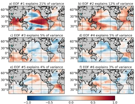
Fig. 3: First six EOFs determined for the same dataset as used to build the H-SST network.
24
Fig. 3. First six EOFs determined for the same data set as used to
build the H-SST network.
preferable to filter out such weakly modular regions because partitioning them into communities could be misleading. Be-cause (i) the detected Infomap partition is less affected by this filtration process than the modularity-based partitions and (ii) the fact that the random walkers in the Infomap algo-rithm are closely related to the flow in a dynamical networks, the Infomap algorithm appears to be the best choice for the study of patterns of climate variability.
Fig. 4: First six varimax-rotated EOFs estimated from the same dataset as used to build the H-SST
network.
25
Fig. 4. First six varimax-rotated EOFs estimated from the same data
set as used to build the H-SST network.
3.2 Communities in the H-SST network: interpretation
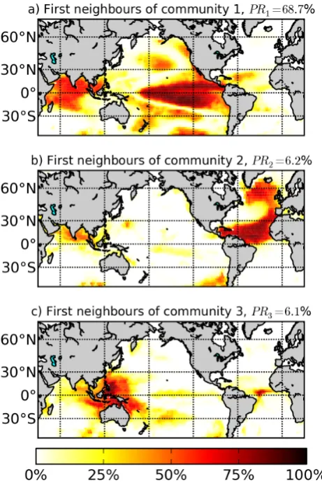
In this section, a physical interpretation of the communities of the H-SST network (Fig. 2b) is given. Community #1 is by far the dominant community in terms of PageRank (69%) and size. Most of the nodes are located in the tropical Pacific but remote patches – located in the Pacific extra-tropics, tropical Indian ocean and northwestern tropical Atlantic – are also part of the community. This result suggests that teleconnec-tions exist between the tropical Pacific and remote regions over the globe. These teleconnections can be deduced from the first neighbours map which is plotted in Fig. 5a for com-munity #1. For each node in the network, this map shows to which percentage of the nodes in the community it is con-nected to. For example, a node in the equatorial Atlantic is connected to about 25% of the nodes in the community.
From Fig. 5a, it can be seen that community #1 is well de-fined (nodes inside the community are connected to most of the other nodes of this community and are only sparsely con-nected to nodes outside the community) and that the differ-ent remote patches of the community are connected to each other. We have verified that the equatorial Pacific nodes are anti-correlated with those of the two small patches located around 30◦in the North and South Pacific and to those near New Zealand, while they are positively correlated with the other nodes of the community. The spatial pattern of the com-munity #1 also coincides with the EOF and R-EOF (Fig. 3a and Fig. 4a, respectively), explaining most of the variance. It also corresponds with the (December–February) El Niño/La Niña composites of HadISST SST determined in Alexander and Bladé (2002) (their Fig. 6a). Thus, these results suggest that community #1 is representative of the dominant pattern of variability on interannual timescales, i.e. ENSO.
The teleconnections shown in Fig. 5a have been described extensively in the literature. Perhaps the most well-known
re-Fig. 5: First neighbours map of communities (a) #1, (b) #2, and (c) #3 in the H-SST network. For
each node, the color scale indicates the percentage of the nodes in the community to which that node
is connected.
26
Fig. 5. First neighbours map of communities (a) #1, (b) #2, and (c)
#3 in the H-SST network. For each node, the color scale indicates the percentage of the nodes in the community to which that node is connected.
mote impacts of ENSO are the changed atmospheric circula-tion over the northern Pacific and North America region and the associated SST anomalies in the North Pacific (Wallace and Gutzler, 1980; Deser and Blackmon, 1995; Lau, 1997). A similar relationship between the tropical and the south Pa-cific (Liu et al., 2002; Ciasto and Thompson, 2008) as well as the warming of the tropical Indian ocean (Lanzante, 1996; Klein et al., 1999) and tropical Atlantic (Curtis and Hasten-rath, 1995; Lanzante, 1996; Enfield and Mayer, 1997; Klein et al., 1999) basins have also been reported. Previous stud-ies suggest that the main mechanism involved in these tele-connections on interannual timescales is the “atmospheric bridge” (Lau and Nath, 1996). This bridge occurs through changes in the Hadley and Walker cells and through the in-teraction of Rossby waves with the quasi-stationary flow and storm tracks (Trenberth et al., 1998; Alexander and Bladé, 2002).
(a)
(b)
Fig. 6: (a) Degree centrality of the H-SST-LP8y network. The network was built using the same
methodology as the H-SST network except that the time series were 8 years low-pass filtered and a
thresholdτ= 0.6was used for significance; this results in an edge densityρ= 0.087. (b) Filtered
communities in the H-SST-LP8y network.
27
Fig. 6. (a) Degree centrality of the H-SST-LP8y network. The
net-work was built using the same methodology as the H-SST netnet-work except that the time series were 8 yr low-pass filtered and a thresh-oldτ=0.6 was used for significance; this results in an edge density ρ=0.087. (b) Filtered communities in the H-SST-LP8y network.
community but the third R-EOF (Fig. 3c) exhibits clear sim-ilarities with it. This spatial pattern bears the signature of the AMO (Guan and Nigam, 2009).
The next community, #3, covers the maritime continent and the Philippine and East China seas, a region below re-ferred to as the Indian Ocean-West Pacific (IWP). The sec-ond R-EOF (Fig. 3b) has a similar pattern as this com-munity although it also shows strong variance in the In-dian ocean. The IWP is located at the confluence of the Pa-cific and Indian Oceans and connects the two oceans by the Indonesian Throughflow (ITF). Ramage (1968) has shown that the IWP is one of the greatest sources of energy for the extratropical circulation. Deep convection takes place in this region and the overlying atmosphere is highly sensi-tive to changes in SST (see Qu et al., 2005 for a review). Interannual variability in this region can be largely under-stood in terms of Kelvin and Rossby waves generated by remote zonal winds along the Indian and Pacific equatorial regions as well as by changes in the volume transport of the Indonesian Throughflow.
Although the other communities (#4–#10) also exhibit similarities with known spatial patterns of variability, we will not discuss this as their PageRank is much lower than the first three communities. For example, communities #8 and #9 are located in the region of the pathways of the northern West-ern Boundary Currents (Qiu, 2000; Frankignoul, 2001) and community #4 appears to connect the southern wind-driven gyres (Speich et al., 2002). The first 6 communities can be as-sociated with the first 6 R-EOFs, however, when more EOFs are rotated, no additional pattern of variability could be iden-tified (not shown here). Hence, the community analysis
al-(c)
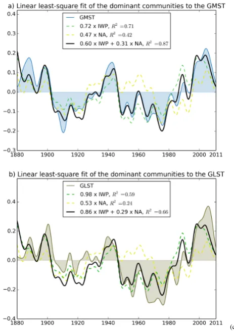
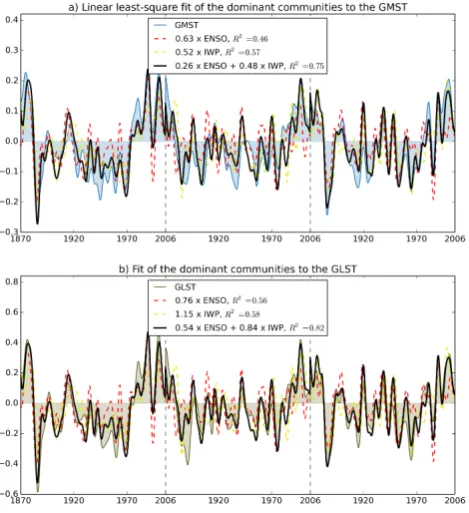
Fig. 7: Regression of the mean time series of the IWP and NA communities of the H-SST-LP8y
network to the (a) GMST and (b) GLST.
28
Fig. 7. Regression of the mean time series of the IWP and NA
communities of the H-SST-LP8y network to the (a) GMST and (b) GLST.
lowed us to detect more detailed features of SST variability represented in the HadISST data set.
4 Decadal SST variability and its connection with the GMST
4.1 Observations
(a)
(b)
Fig. 8: (a) Degree centrality of the ESM-SST network. The network was built using the same
methodology as for the H-SST network but using SST from the MPI-ESM-LR historical simulations.
A thresholdτ= 0.4was used as for the H-SST network leading to an edge densityρ= 0.073. (b)
Filtered communities in the ESM-SST network.
29
Fig. 8. (a) Degree centrality of the ESM-SST network. The network
was built using the same methodology as for the H-SST network but using SST from the MPI-ESM-LR historical simulations. A thresh-oldτ=0.4 was used as for the H-SST network leading to an edge densityρ=0.073. (b) Filtered communities in the ESM-SST net-work.
The degree centrality and the community structure of the H-SST-LP8y network are plotted in Fig. 6a and b, respec-tively. Overall, the spatial patterns appear similar to those of the H-SST network but important differences exist in the tropics. First of all, the degree centralities of the nodes in the H-SST-LP8y network located in the tropical Pacific and Indian ocean have decreased significantly, compared to those in the H-SST network; in the extra-tropics the opposite effect occurs (Fig. 6a). Community #1 (Fig. 6b) of the H-SST-LP8y network (which exhibits a similar pattern as the ENSO com-munity in the H-SST network) has a much lower PageRank (31% versus 69% in the H-SST network). This result is ex-pected when interannual variability and, a fortiori, variability related to ENSO, is filtered out. A second important differ-ence is that the nodes lying in the Indian Ocean are no longer part of the same community as the nodes of the tropical Pa-cific. They are, instead, part of the same community as the nodes in the IWP region (community #2 in the H-SST-LP8y network). Furthermore, this IWP community has a PageR-ank of 26 % which is comparable to the PageRPageR-ank of the tropical Pacific community #1 (31%). The community of the North Atlantic (NA, community #3 in the H-SST-LP8y net-work) and the community of the southern wind-driven gyres (community #4 in the H-SST-LP8y network) also exhibit higher PageRanks (15 and 11%, respectively) than the cor-responding communities in the H-SST network. These high PageRanks (or high number of links) are representative of the strong co-variability of the nodes in these regions on decadal timescales, indicating that important components of decadal variability are present in the IWP region, the NA and the southern wind-driven gyres communities.
(a)
(b)
Fig. 9: (a) Degree centrality of the ESM-SST-LP8y network. The network was built using the
same methodology as for the H-SST-LP8y network but using SST from the MPI-ESM-LR historical
simulations. A threshold ofτ= 0.6was used as for the H-SST network leading to an edge density
ρ= 0.077. (b) Filtered communities in the ESM-SST-LP8y network.
30
Fig. 9. (a) Degree centrality of the ESM-SST-LP8y network. The
network was built using the same methodology as for the H-SST-LP8y network but using SST from the MPI-ESM-LR historical sim-ulations. A threshold ofτ=0.6 was used as for the H-SST network leading to an edge densityρ=0.077. (b) Filtered communities in the ESM-SST-LP8y network.
In order to investigate the relationship between the spa-tial patterns of variability represented by the communities and the global mean state of the climate system, correlations were calculated between mean SST time series associated with each community (in both H-SST and H-SST-LP8y data set) and three indices of global mean surface temperature (GMST). The time series representing the SST of a specific community was calculated by spatially averaging the time series of the nodes of the community. This spatial averag-ing is equivalent to projectaverag-ing the data set on the community vectorsCj of sizeN whereCij equals 1 if nodei belongs to communityj, 0 otherwise. Thus, these community time series are to communities what expansion coefficients are to EOFs.
The Global Surface Temperature Anomalies of the NOAA (Smith and Reynolds, 2005) averaged over land and ocean (GMST), land only (GLST) and ocean only (GOST) were used as indices of the mean state of the climate system. The indices were processed using the same methodology as for the H-SST and H-SST-LP8y data sets (1 and 8 yr, respec-tively, low-pass filtered detrended anomalies) and cover the period 1880–2011. The correlations between the time se-ries of the communities and the indices for the H-SST and H-SST-LP8y networks are presented in Tables 1 and 2, re-spectively. For each correlation, a 95% confidence interval is given in brackets and correlations significant at the 5% level in bold face. The confidence intervals and significance lev-els were estimated using the MBB method as described in Sect. 2.
Fig. 10: Regression of the mean time series of the ENSO and IWP communities of the ESMP-LP8y
network to the (a) GMST and (b) GLST.
31
Fig. 10. Regression of the mean time series of the ENSO and IWP
communities of the ESMP-LP8y network to the (a) GMST and (b) GLST.
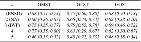
GLST. Only communities #1–#3 and #5 in the H-SST net-work (Table 1) are significantly correlated with the GLST. On decadal timescales (Table 2), the first three communi-ties also show significant correlations with the GLST but the ENSO community (#1) does not display anymore the largest correlation to the GLST and to the GOST (as in the H-SST network). Now the Indian Ocean-West Pacific (IWP) com-munity (#2) and the NA comcom-munity (#3) are best correlated to the GOST with the IWP community displaying largest cor-relations to the GLST. The corcor-relations of 0.77 and 0.84 be-tween the IWP time series of SST and GLST and GMST, respectively, is striking and the IWP region appears to play a major role in decadal climate variability.
Figure 7 represents the linear regressions against the GMST and GLST indices of the time series of the IWP community (#2), the NA community (#3) and of the bivari-ate time series of the IWP and NA communities (multiple-regression) in a least-square sense. The bivariate fits to the GMST and GLST result in coefficients of multiple-determination (a measure of how much the fitted time series determine the original time series, von Storch and Zwiers, 1999b) of 0.87 and 0.66, respectively. This shows that the patterns of both communities can, together, statistically ex-plain most of the decadal variability of the GMST and the largest part of the decadal variability of the GLST. Using the ENSO time series does not significantly improve the fits. However, this analysis is only statistical and no causality be-tween the time series of the communities and the temperature
Table 1. Correlations between the mean time series of the
commu-nities of the H-SST network and the indices of mean, land and ocean surface temperatures (all time series 1y low-pass filtered). The 95 % confidence intervals are given in brackets and correlations signifi-cant at 5 % in italic face.
# GMST GLST GOST
1 (ENSO) 0.66 [0.62, 0.73] 0.44 [0.36, 0.51] 0.71 [0.67, 0.79] 2 (NA) 0.59 [0.43, 0.68] 0.43 [0.19, 0.55] 0.59 [0.47, 0.68] 3 (IWP) 0.50 [0.30, 0.54] 0.44 [0.23, 0.50] 0.45 [0.24, 0.52] 4 0.41 [0.13, 0.50] 0.22[−0.06,0.35] 0.45 [0.21, 0.54] 5 0.42 [0.33, 0.54] 0.30 [0.18, 0.42] 0.43 [0.34, 0.53] 6 0.25 [0.07, 0.40] 0.11[−0.06,0.24] 0.30 [0.11, 0.46] 7 0.26 [0.11, 0.44] 0.11[−0.02,0.21] 0.32 [0.16, 0.52] 8 0.22[0.02,0.35] 0.17[−0.07,0.35] 0.21[0.02,0.32] 9 0.14[−0.18,0.37] 0.07[−0.29,0.35] 0.16[−0.08,0.32] 10 0.27 [0.05, 0.37] 0.07[−0.12,0.18] 0.35 [0.12, 0.45]
Table 2. Correlations between the mean time series of the
com-munities of the H-SST-LP8y network and the indices of mean, land and ocean surface temperatures (all time series 8y low-pass filtered). The 95 % confidence intervals are given in brackets and correlations significant at 5 % in italic face.
# GMST GLST GOST
1 (ENSO) 0.52 [0.36, 0.73] 0.47 [0.28, 0.68] 0.50 [0.33, 0.66]
2 (IWP) 0.84 [0.72, 0.91] 0.77 [0.55, 0.89] 0.78 [0.59, 0.87]
3 (NA) 0.65 [0.38, 0.83] 0.49 [0.06, 0.77] 0.67 [0.43, 0.82]
4 0.55 [0.18, 0.74] 0.28[−0.22,0.56] 0.62 [0.33, 0.78] 5 0.35 [-0.15, 0.59] 0.29[−0.24,0.57] 0.34 [-0.11, 0.56] 6 0.45 [0.18, 0.62] 0.34[0.02,0.59] 0.44 [0.18, 0.61] 7 0.51 [0.30, 0.77] 0.19[−0.06,0.47] 0.63 [0.39, 0.85] 8 0.55 [0.16, 0.69] 0.24[−0.23,0.44] 0.64 [0.25, 0.75]
9 0.12[−0.37,0.49] 0.04[−0.53,0.56] 0.14[−0.27,0.44]
10 −0.14[−0.53,0.29] −0.51[−0.70,−0.12] 0.07[−0.43,0.44]
indices can be stated. Also, the increase in GMST since the 1970s may be explained by the phase synchronization of the time series of the IWP and NA communities, although, once again, the increase of both this index and the time series of the communities could also arise from other factors such as an increased radiative forcing (Fig. 7).
4.2 ESM simulations
1 (ENSO) 0.63 [0.56, 0.67] 0.65 [0.56, 0.69] 0.67 [0.61, 0.71] 2 0.68 [0.58, 0.71] 0.41 [0.25, 0.45] 0.47 [0.32, 0.51]
3 (IWP) 0.42 [0.26, 0.45] 0.38 [0.21, 0.41] 0.38 [0.22, 0.42]
4 0.35 [0.18, 0.41] 0.34 [0.19, 0.40] 0.33 [0.16, 0.40]
5 (NA) 0.44 [0.31, 0.50] 0.44 [0.31, 0.49] 0.49 [0.36, 0.56]
6 −0.05[−0.19,0.01] −0.11[−0.22,−0.03] −0.04[−0.18,0.04]
7 0.31 [0.18, 0.36] 0.33 [0.21, 0.38] 0.30 [0.16, 0.36] 8 0.33 [0.17, 0.38] 0.30 [0.17, 0.35] 0.35 [0.21, 0.39] 9 0.16 [-0.05, 0.23] 0.14 [-0.03, 0.21] 0.13 [-0.08, 0.20] 10 0.16 [0.00, 0.20] 0.18 [0.04, 0.23] 0.14 [-0.02, 0.20] 11 0.14 [-0.15, 0.21] 0.10 [-0.14, 0.19] 0.11[−0.16,0.18] 12 0.40 [0.24, 0.47] 0.39 [0.25, 0.43] 0.43 [0.28, 0.49]
series of one simulation (thus increasing statistical signifi-cance). These model networks will be referred to below as the ESM-SST and ESM-SST-LP8y networks, respectively.
The degree centrality distribution and community struc-ture of the ESM-SST network are plotted in Fig. 8a and b, respectively. Similar to the results for the H-SST network, the ENSO community (#1) and the IWP community (#3) are visible (Fig. 8b) and the ENSO community also domi-nates with a PageRank of 81%. However, only the southern half of the NA community is present (community #5 in Fig. 8b), likely indicative of an under-representation of the AMO-related variability in the model. Also, fewer connections be-tween the ENSO community and the extratropical Pacific are visible (Fig. 8a and b) than in the H-SST network. A weaker atmospheric bridge may be responsible for the absence of such teleconnections. Finally, we can see in Table 3 that the ENSO, IWP and NA communities are, as in the observations, strongly correlated to the GOST and GLST.
For the ESM-SST-LP8y network, the degree distribution and community structure (shown in Fig. 9a and b, respec-tively) are quite similar to those of the ESM-SST network. However, most of the nodes located in the extra-tropics are unassigned, indicative of a weak spatial coherence of the ex-tratropical SST variability. Interestingly, the PageRank of the ENSO community (community #1) is still very high (81%) so that decadal variability is also dominated by the ENSO community. This too strong decadal tropical variability has already been reported by Jungclaus and Keenlyside (2006) for a previous configuration of this model (ECHAM5/MPI-OM). Zanchettin et al. (2012) also showed that the tropical Indian SSTs are over-sensitive to tropical Pacific fluctuations in this model. Decadal variability in the GLST within this ESM can be largely explained (statistically) by the ENSO and IWP communities (Fig. 10), but misses the connection to the NA as found in the observations (Table 4). Contrary to Fig. 7, the fits in Fig. 10 were made without the time series
1 (ENSO) 0.68 [0.51, 0.74] 0.75 [0.60, 0.80] 0.68 [0.50, 0.73] 2 (NA) 0.60 [0.36, 0.67] 0.66 [0.44, 0.73] 0.62 [0.38, 0.70] 3 (IWP) 0.75 [0.55, 0.77] 0.75 [0.55, 0.78] 0.69 [0.46, 0.72] 4 0.77 [0.55, 0.80] 0.63 [0.29, 0.67] 0.62 [0.30, 0.67] 5 0.46 [0.13, 0.52] 0.48 [0.21, 0.53] 0.48 [0.18, 0.54]
of the NA community, the regressions were not significantly improved using this time series.
To conclude, the main aspects of the SST variability found in the observations are also visible in the MPI-ESM-LR model but the variability related to ENSO (NA) is over-represented (under-over-represented). These model biases could be efficiently identified using the network approach.
5 Summary and discussion
In order to study the global climate variability, we have an-alyzed SST observations and ESM simulations using a cli-mate network approach focusing on the detection of commu-nities. The network techniques provide an innovative and ef-ficient complementary approach to more traditional methods like EOF analysis, composite analysis and correlation maps. An EOF analysis is usually efficient in detecting the domi-nant mode of variability but the secondary modes, being con-strained to be orthogonal to the first one, are less likely to rep-resent regional patterns of variability (Monahan et al., 2009). Thus, when applying an EOF analysis on the HadISST SST data over the globe, only the first EOF can be attributed to a physical pattern of climate variability, namely ENSO, while the higher EOF modes could not be connected to any known patterns of variability. This shortcoming can be by-passed by rotating the EOFs like was done by Kawamura (1994). However, one of the drawbacks of this method is that the re-sults are sensitive to the choice of the rotation criterion, to the choice of the number of loadings and to the normalization of the EOFs (von Storch and Zwiers, 1999a).
must subsequently be applied to distribute the nodes into dis-tinct groups of co-varying nodes.
Detecting communities in the HadISST and MPI-ESM networks was more efficient in revealing non-overlapping spatial patterns of SST variability than EOF analysis. We have indeed shown in Sect. 3 that most of the communities in the H-SST network (Fig. 2) can be associated to known phys-ical patterns of variability, which could not have been done using a regular EOF analysis on the global oceans. More pat-terns could be found using 6 rotated EOFs but the choice of the number of loadings could only be done by evaluating the correspondence of the rotated EOFs with the communi-ties. However, the main drawback of the Infomap community detection algorithm is that it is not able to detect overlap-ping spatial patterns of variability. For example, we can see from Fig. 5 that the nodes in the Caribbean Sea associated with the second community (NA) could also be associated with the first community (ENSO) which was also suggested by Guan and Nigam (2009). Overlapping community detec-tion algorithms exist (e.g. Shen et al., 2009; Lancichinetti et al., 2009), however, because of their complex implemen-tation and slower execution application of these techniques are outside the scope of this study.
By augmenting the community analysis with first neigh-bours maps (Fig. 5), teleconnections and links between com-munities can be revealed. The study of these maps offers several advantages over correlation maps or composites. The main interest of the network approach is that neither a sta-tistical event nor an index has to be defined a priori. For ex-ample, the results obtained using the first neighbours of the ENSO community in the H-SST network (Fig. 5a) are sim-ilar to those of Alexander and Bladé (2002) using compos-ites, but we did not need to define what El Niño and La Niña events represent statistically. Correlation maps obtained by Klein et al. (1999) and Alexander and Bladé (2002) are also similar to Fig. 5a, but once again, we did not need to define over which domain to spatially average to obtain the relevant time series. In short, using community detection algorithms neither prior information nor a choice of a pattern of vari-ability to be studied is necessary, making pioneering studies easier and maybe also less biased.
The community structure of the H-SST network (Fig. 2) proved to be in good agreement with known spatial pat-terns of climate variability, further supporting the use of this method to identify climate patterns of variability from large gridded data sets. On interannual timescales, the main com-munity could be associated with the dominant pattern of vari-ability, ENSO and its remote influences were visible as part of the community or in the first neighbours maps. These tele-connections could in part be interpreted using the “atmo-spheric bridge” concept. Other patterns of variability, such as the AMO, were also visible as independent components of the system.
One of the key differences between the H-SST and the H-SST-LP8y networks is that the Indian Ocean-West
Pa-cific (IWP) region appears an independent and strongly intra-connected community in the H-SST-LP8y network whereas its western part is connected to the tropical Pacific in the H-SST network. This suggests that decadal variability in the IWP region is not driven by tropical Pacific variability through the atmospheric bridge as on interannual timescales. Furthermore, a large component of the observed global land surface temperature (GLST) variability can be explained by the time series associated with the IWP community.
To infer whether the IWP SST drives or responds to decadal variability of the overlying atmosphere is a difficult problem, since little is known about the sources of such low-frequency variability in the climate system. Several argu-ments support the idea that SST decadal variability can drive land surface temperature (LST) changes. First, the maximum cross-correlation of the time series associated to the IWP community in the H-SST-LP8y network and the GLST in-dex is found for the IWP time series leading the GLST of 18 months, although significant correlations are also found for lags ranging from −240 months (IWP leading) to 77 months (GLST leading). Secondly, Dommenget (2009) sug-gests, using observations and GCM simulations, that the “ocean’s variability is leading to variability with enhanced magnitude over the continents, causing much of the longer timescale (decadal) global-scale continental climate variabil-ity”. In particular, several studies show that decadal SST fluc-tuations in the IWP region may influence the East Asian Monsoon (Hu, 1997; Zhou et al., 2009) through changes in the West Pacific subtropical high. Zhang et al. (2004) suggest that the warming of the IWP region can lead to enhanced pre-cipitation over the Tibetan Plateau and that the resulting creased snow cover over the plateau in spring can further in-duce changes in circulation and precipitation over East Asia during the subsequent summer. Consequently, the Asian con-tinent appears to be very sensitive to SST fluctuations in the IWP region.
vations as well as its influence on the tropical Indian Ocean basin. On the other hand, other patterns such as the NA are much weaker than in observations. Most of the extratropi-cal nodes of the network are unassigned, indicative of a low coherence in the simulated SSTs. However, we also found a strong relationship between the IWP region and the GLST, which is in agreement with that found the observations. How the IWP region and the GLST interact in the model needs further investigation but is outside the scope of this paper.
Acknowledgements. The authors would like to acknowledge
the support of the LINC project (no. 289447) funded by EC’s Marie-Curie ITN program (FP7-PEOPLE-2011-ITN).
Edited by: D. Kirk-Davidoff
References
Alexander, M. A. and Bladé, I.: The atmospheric bridge: The in-fluence of ENSO teleconnections on air-sea interaction over the global oceans, J. Am. Meteorol. Soc., 15, 2205–2231, 2002. Arenas, A., Díaz-Guilera, A., and Pérez-Vicente, C. J.:
Synchro-nization reveals topological scales in complex networks, Phys. Rev. Lett., 96, 114102, doi:10.1103/PhysRevLett.96.114102, 2006.
Balmaseda, M. A., Trenberth, K. E., and Källén, E.: Distinctive cli-mate signals in reanalysis of global ocean heat content, Geophys. Res. Lett., 40, 1754–1759, doi:10.1002/grl.50382, 2013. Barthélemy, M.: Spatial networks, Physics Reports, 499, 1–101,
doi:10.1016/j.physrep.2010.11.002, 2011.
Bindoff, N., McDougall, T., Crc, A., and Division, C.: Decadal Changes along an Indian Ocean Section at 32 S and Their In-terpretation, J. Phys. Oceanogr., 30, 1207–1222, 2000.
Blondel, V. D., Guillaume, J.-L., Lambiotte, R., and Lefeb-vre, E.: Fast unfolding of communities in large networks, J. Stat. Mechan.: Theory and Experiment, 2008, P10008, doi:10.1088/1742-5468/2008/10/P10008, 2008.
Brin, S. and Page, L.: The anatomy of a large-scale hypertextual Web search engine, Computer Networks and ISDN Systems, 30, 107–117, doi:10.1016/S0169-7552(98)00110-X, 1998.
Canty, T., Mascioli, N. R., Smarte, M. D., and Salawitch, R. J.: An empirical model of global climate – Part 1: A critical evalua-tion of volcanic cooling, Atmos. Chem. Phys., 13, 3997–4031, doi:10.5194/acp-13-3997-2013, 2013.
Ciasto, L. M. and Thompson, D. W. J.: Observations of Large-Scale Ocean-Atmosphere Interaction in the Southern Hemisphere, J. Climate, 21, 1244–1259, doi:10.1175/2007JCLI1809.1, 2008. Costa, L. and Rodrigues, F.: Characterization of complex networks:
A survey of measurements, Adv. Phys., 56, 167–242, 2007.
cal and North Pacific Sea Surface Temperature Variations, J. Cli-mate, 8, 1677–1680, 1995.
Deser, C., Alexander, M. A., Xie, S.-P., and Phillips, A. S.: Sea Surface Temperature Variability: Patterns and Mechanisms, Annu. Rev. Mar. Sci., 2, 115–143, doi:10.1146/annurev-marine-120408-151453, 2010.
Dommenget, D.: The Ocean’s Role in Continental Cli-mate Variability and Change, J. CliCli-mate, 22, 4939–4952, doi:10.1175/2009JCLI2778.1, 2009.
Dommenget, D. and Latif, M.: Generation of hyper climate modes, Geophys. Res. Lett., 35, L02706, doi:10.1029/2007GL031087, 2008.
Donges, J. F., Zou, Y., Marwan, N., and Kurths, J.: Complex net-works in climate dynamics, The European Phys. J. Special Top-ics, 174, 157–179, doi:10.1140/epjst/e2009-01098-2, 2009a. Donges, J. F., Zou, Y., Marwan, N., and Kurths, J.: The backbone
of the climate network, EPL (Europhysics Letters), 87, 48007, doi:10.1209/0295-5075/87/48007, 2009b.
Donges, J. F., Schultz, H. C. H., Marwan, N., Zou, Y., and Kurths, J.: Investigating the topology of interacting networks, The European Phys. J. B, 84, 635–651, doi:10.1140/epjb/e2011-10795-8, 2011. Duchon, C.: Lanczos filtering in one and two dimensions, J. Appl.
Meteorol., 18, 1016–1022, 1979.
Enfield, D.: The Atlantic multidecadal oscillation and its relation to rainfall and river flows in the continental US, Geophys. Res. Lett., 28, 2077–2080, 2001.
Enfield, D. and Mayer, D.: Tropical Atlantic sea surface temperature variability relation to El Nino-Southern Oscillation, J. Geophys. Res., 102, 929–945, 1997.
Foster, G. and Rahmstorf, S.: Global temperature evolution 1979–2010, Environ. Res. Lett., 6, 044022, doi:10.1088/1748-9326/6/4/044022, 2011.
Frankignoul, C.: Gulf Stream Variability and Ocean-Atmosphere Interactions*, J. Phys. Oceanogr., 31, 3516–3529, 2001. Gozolchiani, A., Yamasaki, K., Gazit, O., and Havlin, S.: Pattern of
climate network blinking links follows El Niño events, EPL (Eu-rophysics Letters), 83, 28005, doi:10.1209/0295-5075/83/28005, 2008.
Gozolchiani, A., Havlin, S., and Yamasaki, K.: Emer-gence of El Niño as an Autonomous Component in the Climate Network, Phys. Rev. Lett., 107, 1–5, doi:10.1103/PhysRevLett.107.148501, 2011.
Guan, B. and Nigam, S.: Analysis of Atlantic SST Variability Fac-toring Interbasin Links and the Secular Trend: Clarified Structure of the Atlantic Multidecadal Oscillation, J. Climate, 22, 4228– 4240, doi:10.1175/2009JCLI2921.1, 2009.
Hasselmann, K.: Stochastic climate models Part I. Theory, Tellus, 28, 473–485, doi:10.1111/j.2153-3490.1976.tb00696.x, 1976. Hu, Z.-Z.: Interdecadal variability of summer climate over
Jungclaus, J. H. and Keenlyside, N.: Ocean circulation and tropical variability in the coupled model ECHAM5/MPI-OM, J. Climate, 19, 3952–3972, 2006.
Jungclaus, J. H., Fischer, N., Haak, H., Lohmann, K., Marotzke, J., Matei, D., Mikolajewicz, U., Notz, D., and von Storch, J.: Char-acteristics of the ocean simulations in MPIOM, the ocean compo-nent of the MPI-Earth system model, J. Adv. Model. Earth Syst., 5, 422–446, doi:10.1002/jame.20023, 2013.
Kaiser, H.: THE VARIMAX CRITERION FOR ANALYTIC RO-TATION IN FACTOR ANALYSIS, Psychometrika, 23, 187– 200, 1958.
Kawamura, R.: A rotated eof analysis of global sea surface tem-perature variability with interannual interdecadal scales, J. Phys. Oceanogr., 24, 707–715, 1994.
Kistler, R., Kalnay, E., and Collins, W.: The NCEP-NCAR 50-year reanalysis: Monthly means CD-ROM and documentation, B. Am. Meteorol. Soc., 82, 247–268, 2001.
Klein, S., Soden, B., and Lau, N.: Remote sea surface temperature variations during ENSO: Evidence for a tropical atmospheric bridge, J. Climate, 12, 917–932, 1999.
Lancichinetti, A. and Fortunato, S.: Community detection al-gorithms: A comparative analysis, Phys. Rev. E, 80, 1–11, doi:10.1103/PhysRevE.80.056117, 2009.
Lancichinetti, A., Fortunato, S., and Kertész, J.: Detecting the overlapping and hierarchical community structure in com-plex networks, New J. Phys., 11, 033015, doi:10.1088/1367-2630/11/3/033015, 2009.
Lanzante, J.: Lag Relationship Involving Sea Surface Temperatures, J. Climate, 9, 2568–2578, 1996.
Lau, N.-C.: Interactions between Global SST Anoma-lies and the Midlatitude Atmospheric Circulation, B. Am. Meteorol. Soc., 78, 21–33, doi:10.1175/1520-0477(1997)078<0021:IBGSAA>2.0.CO;2, 1997.
Lau, N.-C. and Nath, M.: The Role of the “Atmospheric Bridge” in Linking Tropical Pacific ENSO Events to Extratropical SST Anomalies, J. Climate, 9, 2036–2057, 1996.
Lee, T.: Decadal weakening of the shallow overturning circulation in the South Indian Ocean, Geophys. Res. Lett., 31, L18305, doi:10.1029/2004GL020884, 2004.
Liu, J., Yuan, X., Rind, D., and Martinson, D.: Mechanism study of the ENSO and southern high latitude climate teleconnections, Geophys. Res. Lett., 29, 8–11, 2002.
McDonagh, E. and Bryden, H.: Decadal changes in the South Indian Ocean thermocline, J. Climate, 18, 1575–1590, doi:10.1175/JCLI3350.1, 2005.
Mcphaden, M. J., Busalacchi, J., Cheney, R., Gage, S., Halpern, D., Ji, M., Julian, P., Mitchurn, G. T., Niiler, P. P., and Smith, N.: The Tropical Ocean-Global Atmosphere observing system: A decade of progress, J. Geophys. Res., 103, 14169–14240, 1998. Monahan, A. H., Fyfe, J. C., Ambaum, M. H. P.,
Stephen-son, D. B., and North, G. R.: Empirical Orthogonal Func-tions: The Medium is the Message, J. Climate, 22, 6501–6514, doi:10.1175/2009JCLI3062.1, 2009.
Mudelsee, M.: Climate Time Series Analysis: Classical Statistical and Bootstrap Methods, Springer, Atmospheric Edn., 2010. Muller, R. A., Curry, J., Groom, D., Jacobsen, R.,
Perl-mutter, S., Rohde, R., Rosenfeld, A., Wickham, C., and Wurtele, J.: Decadal Variations in the Global Atmospheric
Land Temperatures, J. Geophys. Res.-Atmos., 118, 5280–5286, doi:10.1002/jgrd.50458, 2013.
Newman, M. E. J.: Finding community structure in networks us-ing the eigenvectors of matrices, Phys. Rev. E, 74, 036104, doi:10.1103/PhysRevE.74.036104, 2006.
Newman, M. E. J. and Girvan, M.: Finding and evaluating community structure in networks, Phys. Rev. E, 69, 1–15, doi:10.1103/PhysRevE.69.026113, 2004.
Qiu, B.: Interannual variability of the Kuroshio Extension system and its impact on the wintertime SST field, J. Phys. Oceanogr., 30, 1486–1502, 2000.
Qu, T., Du, Y., Strachan, J., Meyers, G., and Slingo, J.: Sea Sur-face Temperature and its Variability in the Indonesian Region, Oceanography, 18, 50–61, 2005.
Ramage, C.: ROLE O F A TROPICAL – MARITIME CON-TINENT – IN THE ATMOSPHERIC CIRCULATION, Mon. Weather Rev., 96, 365–370, 1968.
Rayner, N. A.: Global analyses of sea surface temperature, sea ice, and night marine air temperature since the late nineteenth cen-tury, J. Geophys. Res., 108, 4407, doi:10.1029/2002JD002670, 2003.
Rosvall, M. and Bergstrom, C.: An information-theoretic frame-work for resolving community structure in complex netframe-works, Proc. Natl. Acad. Sci. USA, 104, 7327–7331, 2007.
Shen, H., Cheng, X., Cai, K., and Hu, M.-B.: Detect over-lapping and hierarchical community structure in net-works, Physica A: Stat. Mechan. Appl., 388, 1706–1712, doi:10.1016/j.physa.2008.12.021, 2009.
Smith, T. and Reynolds, R.: A global merged land-air-sea surface temperature reconstruction based on histori-cal observations (1880–1997), J. Climate, 18, 2021–2036, doi:10.1175/JCLI3362.1, 2005.
Speich, S., Blanke, B., and Vries, P. D.: Tasman leakage: A new route in the global ocean conveyor belt, Geophys. Res. Lett., 29, 1–4, 2002.
Srokosz, M., Baringer, M., Bryden, H., Cunningham, S., Delworth, T., Lozier, S., Marotzke, J., and Sutton, R.: Past, Present, and Fu-ture Changes in the Atlantic Meridional Overturning Circulation, B. Am. Meteorol. Soc., 93, 1663–1676, doi:10.1175/BAMS-D-11-00151.1, 2012.
Stevens, B. and Giorgetta, M.: The atmospheric component of the MPI – earth system model: ECHAM6, Earth Systems, 5, 1–83, 2013.
Sutton, R. T. and Hodson, D. L. R.: Atlantic Ocean forcing of North American and European summer climate, Science (New York, N.Y.), 309, 115–118, doi:10.1126/science.1109496, 2005. Sutton, R. T., Dong, B., and Gregory, J. M.: Land/sea warming
ra-tio in response to climate change: IPCC AR4 model results and comparison with observations, Geophys. Res. Lett., 34, L02701, doi:10.1029/2006GL028164, 2007.
Taylor, K. E., Stouffer, R. J., and Meehl, G. A.: An Overview of CMIP5 and the Experiment Design, B. Am. Meteorol. Soc., 93, 485–498, doi:10.1175/BAMS-D-11-00094.1, 2012.
Trenberth, K.: The definition of el nino, B. Am. Meteorol. Soc., 78, 2771–2777, 1997.
doi:10.1103/PhysRevLett.100.228502, 2008.
Tsonis, A. A., Swanson, K., and Kravtsov, S.: A new dynamical mechanism for major climate shifts, Geophys. Res. Lett., 34, 1– 5, doi:10.1029/2007GL030288, 2007.
Tsonis, A. A., Swanson, K. L., and Wang, G.: On the Role of Atmo-spheric Teleconnections in Climate, J. Climate, 21, 2990–3001, doi:10.1175/2007JCLI1907.1, 2008.
Tsonis, A. A., Wang, G., Swanson, K. L., Rodrigues, F. a., and Costa, L. D. F.: Community structure and dynamics in climate networks, Clim. Dynam., 37, 933–940, doi:10.1007/s00382-010-0874-3, 2010.
Valsala, V., Maksyutov, S., and Murtugudde, R.: Possible inter-annual to interdecadal variabilities of the Indonesian through-flow water pathways in the Indian Ocean, J. Geophys. Res., 115, C10016, doi:10.1029/2009JC005735, 2010.
von Storch, H. and Zwiers, F. W.: Empirical Orthogonal Functions, in: Statistical Analysis in Climate Research, Chap. 13, 293–316, Cambridge University Press, 1999a.
von Storch, H. and Zwiers, F. W.: Regression, in: Statistical Anal-ysis in Climate Research, Chap. 8, 145–169, Cambridge Univer-sity Press, 1999b.
Wallace, J. and Gutzler, D. S.: Teleconnections in the geopoten-tial height field during the northern hemisphere winter, Mon. Weather Rev., 109, 784–812, 1980.
Oscillation and Northern Hemisphere’s climate variability, Clim. Dynam., 38, 929–949, doi:10.1007/s00382-011-1071-8, 2011. Yamasaki, K., Gozolchiani, A., and Havlin, S.: Climate Networks
around the Globe are Significantly Affected by El Niño, Phys. Rev. Lett., 100, 1–4, doi:10.1103/PhysRevLett.100.228501, 2008.
Zanchettin, D., Rubino, a., Matei, D., Bothe, O., and Jungclaus, J. H.: Multidecadal-to-centennial SST variability in the MPI-ESM simulation ensemble for the last millennium, Clim. Dy-nam., 40, 1301–1318, doi:10.1007/s00382-012-1361-9, 2012. Zhang, Y., Li, T., and Wang, B.: Decadal Change of the Spring Snow
Depth over the Tibetan Plateau: The Associated Circulation and Influence on the East Asian Summer Monsoon*, J. Climate, 17, 2780–2793, 2004.