Nonlin. Processes Geophys., 19, 95–111, 2012 www.nonlin-processes-geophys.net/19/95/2012/ doi:10.5194/npg-19-95-2012
© Author(s) 2012. CC Attribution 3.0 License.
Nonlinear Processes
in Geophysics
Spatial patterns of linear and nonparametric long-term trends in
Baltic sea-level variability
R. V. Donner1, R. Ehrcke1, S. M. Barbosa2, J. Wagner1, J. F. Donges1,3, and J. Kurths1,3,4 1Potsdam Institute for Climate Impact Research, P.O. Box 60 12 03, 14412 Potsdam, Germany 2Instituto Dom Luiz, University of Lisbon, Campo Grande, Edif´ıcio C8, 1749-016 Lisboa, Portugal 3Department of Physics, Humboldt University Berlin, Newtonstr. 15, 12489 Berlin, Germany
4Institute for Complex Systems and Mathematical Biology, University of Aberdeen, Aberdeen AB243UE, UK Correspondence to: R. V. Donner ([email protected])
Received: 7 October 2011 – Revised: 6 February 2012 – Accepted: 6 February 2012 – Published: 13 February 2012
Abstract. The study of long-term trends in tide gauge data is important for understanding the present and future risk of changes in sea-level variability for coastal zones, particularly with respect to the ongoing debate on climate change im-pacts. Traditionally, most corresponding analyses have ex-clusively focused on trends in mean sea-level. However, such studies are not able to provide sufficient information about changes in the full probability distribution (especially in the more extreme quantiles). As an alternative, in this paper we apply quantile regression (QR) for studying changes in arbi-trary quantiles of sea-level variability. For this purpose, we chose two different QR approaches and discuss the advan-tages and disadvanadvan-tages of different settings. In particular, traditional linear QR poses very restrictive assumptions that are often not met in reality. For monthly data from 47 tide gauges from along the Baltic Sea coast, the spatial patterns of quantile trends obtained in linear and nonparametric (spline-based) frameworks display marked differences, which need to be understood in order to fully assess the impact of fu-ture changes in sea-level variability on coastal areas. In gen-eral, QR demonstrates that the general variability of Baltic sea-level has increased over the last decades. Linear quan-tile trends estimated for sliding windows in time reveal a wide-spread acceleration of trends in the median, but only localised changes in the rates of changes in the lower and up-per quantiles.
1 Introduction
Global sea-level rise is one of the most direct expected con-sequences of climate change and associated with substan-tial socio-economic risks (IPCC, 2007; Church et al., 2010).
Not only the uncertainty on the future rate of global level rise is very large (e.g. Milne et al., 2009), but also sea-level change is subject to considerable spatial heterogene-ity. As demonstrated by satellite altimetry observations (e.g. Cazenave and Nerem, 2004), sea-level exhibits significant re-gional variability, reflecting the variety of rere-gional and local geophysical phenomena that determine changes in the mass and volume of the Earth’s oceans.
Regional sea-level variability, rather than global sea-level rise, is the main concern for risk assessment. The threat to coastal populations results from the combination of global sea-level rise with regional changes in sea-level associated with changes in atmospheric patterns and winds, tidal ranges, waves, coastal morphology, or land elevation (IPCC, 2007).
96 R. V. Donner et al.: Linear and nonparametric long-term trends in Baltic sea-level variability
Studies of long-term sea-level variability based on the analysis of tide gauge records traditionally assume trends to be linear, and obtainable from the ordinary least squares fit of a first-order polynomial (linear function) to the tide gauge observations. However, among other issues such as auto-correlation (e.g. Barbosa et al., 2008), the assumption of a linear monotonic trend can be highly questionable, particu-larly in the case of strong inter-annual and decadal variability (e.g. Holgate, 2007). Furthermore, slopes derived from linear trend models only provide information on the rate of change of the mean tide gauge observations, whereas long-term vari-ability in other parts of the data distribution is equally or even more relevant, particularly in terms of risk assessment and coastal protection. In this work quantile regression is applied to derive information on long-term variability for the entire probability distribution of sea-level.
This paper is organised as follows: in Sects. 2 and 3, we describe the data and methods considered in this work in some detail. The results of our analysis are presented and thoroughly discussed in Sect. 4. Finally, the main findings of this study are summarised and put into an oceanographic and climate change context (Sect. 5).
2 Baltic tide gauge data
The longest available observational records of sea-level vari-ability are from coastal tide gauge stations. Since tide gauges measure relative sea-level (RSL, i.e. the height of the sea sur-face relative to a reference point on land), these records in-clude both the rise and drop of the sea surface as well as the vertical movements (uplift or subsidence) of the adja-cent land. The interest in studying the postglacial rebound of Fennoscandia motivated the precocious set-up of a dense network of tide gauges in the Baltic area, and as a result a significant number of long and continuous tide gauge records are presently available for studies of long-term sea-level vari-ability.
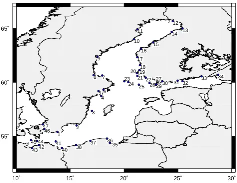
Monthly tide gauge records of relative sea-level are provided by the Permanent Service for Mean Sea Level (PSMSL, see http://www.psmsl.org) (Woodworth and Player, 2003). In this work, we have selected 47 records from the Baltic Sea area with sufficiently continuous data, which are shown in Fig. 1 (for detailed information on the properties of these records, see Table 1). Among these tide gauges, 30 time series provide a sufficiently complete tem-poral coverage of the second half of the 20th century (1951– 1999). Since the data have been obtained from its repository, the basic quality-control procedures defined by the PSMSL have already been applied. For most records only a few non-consecutive observations have been missing, and the total amount of missing values is less than 2 %, as can be seen from Table 1. For a few records (specifically RAA, VAA, LYP, DEG and RUS) one complete year is missing. For one single record (SAS) more than one consecutive year is
2 R.V. Donner et al.: Spatial patterns of linear and nonparametric long-term trends in Baltic sea-level variability
10˚ 15˚ 20˚ 25˚ 30˚
55˚ 60˚ 65˚ 1 2 3 4 5 6 7 8 9 10 11 12 13 14 15 16 17 18 19 20 21 22 23 24 25 26 27 28 2930 31 32
33 34 35 36 37 38 39 40 41 42 43 44 45 46 47
Fig. 1. Location of the tide gauges considered in this study (cf. Tab. 1).
in the case of strong inter-annual and decadal variability (e.g. Holgate (2007)). Furthermore, slopes derived by linear trend models only provide information on the rate of change of the mean of the tide gauge observations, whereas long-term variability in other parts of the data distribution is equally or even more relevant, particularly in terms of risk assessment and coastal protection. In this work quantile regression is ap-plied to derive information on long-term variability for the entire probability distribution of sea-level.
This paper is organised as follows: In Sects. 2 and 3, we describe the data and methods considered in this work in some detail. The results of our analysis are presented and thoroughly discussed in Sect. 4. Finally, the main findings of this study are summarised and put into an oceanographic and climate change context (Sect. 5).
2 Baltic tide gauge data
The longest available observational records of sea-level vari-ability are from coastal tide gauge stations. Since tide gauges measure relative sea-level (RSL, i.e., the height of the sea surface relative to a reference point on land), these records include both the rise and drop of the sea surface as well as the vertical movements (uplift or subsidence) of the adja-cent land. The interest in studying the postglacial rebound of Fennoscandia motivated the precocious set-up of a dense network of tide gauges in the Baltic area, and as a result a significant number of long and continuous tide gauge records are presently available for studies of long-term sea-level vari-ability.
Monthly tide gauge records of relative sea-level are provided by the Permanent Service for Mean Sea Level (PSMSL, see http://www.psmsl.org) (Woodworth and Player, 2003). In this work, we have selected 47 records from
the Baltic Sea area with sufficiently continuous data, which are shown in Fig. 1 (for detailed information on the properties of these records, see Tab. 1). Among these tide gauges, 30 time series provide a sufficiently complete temporal coverage of the second half of the 20th century (1951-1999).Since the data have been obtained from its repository, the basic quality-control procedures defined by the PSMSL have already been applied. For most records only a few non-consecutive obser-vations have been missing, and the total amount of missing values is less than 2%, as can be seen from Tab. 1. For a few records (specifically RAA, VAA, LYP, DEG and RUS) one complete year is missing. For one single record (SAS) more than one consecutive year is missing (1988-1992). However, gaps in the monthly time series data need not to be filled in, since quantile regression (see Sect. 3) as the method of choice in this work does not require equidistant observations and is thus able to cope with missing observations.
As it can be seen from Tab. 1, a large part of the Baltic region experiences a notable land uplift due to postglacial rebound, reaching∼9mm/year in the northern area of the Gulf of Bothnia (e.g., Ekman (1996)). In this work, the up-lift effect is considered in terms of a glacial isostatic adjust-ment (GIA) model based on the VM4 earth model (Peltier, 1998, 2004). Corresponding average trends in relative sea-level have also been obtained from the PSMSL.In turn, the tide gauge records under study have not been corrected for the inverse barometric effect, since we are interested in in-vestigating the observed sea level variability in the Baltic sea as such, irrespective of the causative forcings, atmospheric or other.
Sea-level in the Baltic exhibits in general an annual cy-cle peaking in the winter months (e.g. H¨unicke and Zorita (2008)). For the purpose of studying long-term sea-level variability, the mean annual cycle is estimated by averaging all values for each calender month contained in the respective time series, and then subtracted from each sea-level record. For this purpose, we have used the STL ((S)easonal-(T)rend decomposition procedure based on (L)ocally weighted re-gression) algorithm (Cleveland et al., 1990) for a seasonal time series decomposition by means of locally weighted re-gression (LOESS) (Cleveland, 1979; Cleveland and Devlin, 1988) in its implementation in theRpackagestats. For simplicity, we considered a fixed seasonal cycle instead of a potentially changing one, which might provide an even more appropriate description of the corresponding annual variabil-ity component. Note that the proper removal of all sea-sonal effects is a non-trivial and still not completely solved problem of geoscientific time series analysis (Donner et al., 2008). In general, the results of quantile regression depend to some degree on whether or not seasonality effects have been removed from the data prior to analysis (see Sect. 4.1).In or-der to further address the related problems, it would be neces-sary to systematically compare the performance of different methods for removing the annual cycle from the data in order to verify the robustness of the obtained results of quantile
re-Fig. 1. Location of the tide gauges considered in this study (cf.
Table 1).
missing (1988–1992). However, gaps in the monthly time series data need not to be filled in, since quantile regression (see Sect. 3) as the method of choice in this work does not require equidistant observations and is thus able to cope with missing data.
As it can be seen from Table 1, a large part of the Baltic region experiences a notable land uplift due to postglacial re-bound, reaching∼90 mm dec−1in the northern area of the Gulf of Bothnia (e.g. Ekman, 1996). In this work, the up-lift effect is considered in terms of a glacial isostatic adjust-ment (GIA) model based on the VM4 earth model (Peltier, 1998, 2004). Corresponding average trends in relative sea-level have also been obtained from the PSMSL. In turn, the tide gauge records under study have not been corrected for the inverse barometric effect, since we are interested in in-vestigating the observed sea-level variability in the Baltic sea as such, irrespective of the causative forcings, atmospheric or other.
R. V. Donner et al.: Linear and nonparametric long-term trends in Baltic sea-level variability 97
Table 1. Basic properties of the tide gauge records used in this study. The station ID refers to the coastline (first three digits) and station
codes from the PSMSL.T,Nand NA give the total length of the time series (in years), the number of data points, and the number of missing data points, respectively, LON and LAT denote the station coordinates. GIA-VM4 lists the average trends in sea-level due to glacial isostatic adjustment obtained from the VM4 earth model (see http://www.psmsl.org/train and info/geo signals/gia/peltier/).
ID Station Observation T N NA LON LAT GIA–VM4
Period (yr) (◦E) (◦N) (mm dec−1)
1 050071 Ystad Jan 1887–Dec 1981 95 1140 0 13.817 55.417 2.4
2 050081 Kungholmsfort Jan 1887–Dec 2006 120 1440 1 15.583 56.01 1.6 3 050091 Olands Norra Udde Jan 1887–Dec 2006 120 1440 0 17.01 57.367 −2.9 4 050121 Landsort Jan 1887–Dec 2006 120 1440 0 17.867 58.75 −16.1 5 050131 Nedre Sodertalje Jan 1869–Dec 1970 102 1224 0 17.617 59.2 −23.1 6 050141 Stockholm Jan 1889–Dec 2006 118 1416 0 18.083 59.317 −23.5
7 050161 Bjorn Jan 1892–Dec 1976 85 1020 0 17.967 60.633 −44.2
8 050171 Nedre Gavle Jan 1896–Dec 1986 91 1092 1 17.167 60.667 −45.9
9 050183 Spikarna Jan 1969–Dec 2006 38 456 1 17.533 62.367 −58.8
10 050191 Ratan Jan 1892–Dec 2006 115 1380 3 20.917 64 −70.7
11 050210 Furuogrund Jan 1916–Dec 2006 91 1092 5 21.233 64.9167 −73.9
12 060001 Kemi Jan 1920–Dec 2004 85 1020 40 24.5167 65.667 −81.8
13 060011 Oulu Jan 1889–Dec 2004 116 1392 68 25.4167 65.0033 −79.1
14 060021 Raahe Jan 1923–Dec 2004 82 984 75 24.4167 64.667 −79.0
15 060041 Pietarsaari Jan 1915–Dec 2004 90 1080 21 22.7 63.7 −69.9
16 060051 Vaasa Jan 1922–Dec 2004 83 996 75 21.567 63.1 −64.3
17 060071 Kaskinen Jan 1927–Dec 2004 78 936 23 21.2167 62.333 −56.1 18 060101 Mantyluoto Jan 1911–Dec 2004 94 1128 19 21.467 61.6 −44.7
19 060121 Rauma Jan 1933–Dec 2004 72 864 6 21.4333 61.1333 −37.6
20 060221 Lyokki Jan 1858–Dec 1936 79 948 3 21.1833 60.85 −34.6
21 060231 Lypyrtti Jan 1858–Dec 1936 79 948 17 21.2333 60.6 −30.2
22 060241 Turku Jan 1922–Dec 2004 83 996 21 22.01 60.433 −22.4
23 060271 Lemstrom Jan 1889–Dec 1936 48 576 0 20.0167 60.1 −28.6
24 060281 Degerby Jan 1924–Dec 2004 81 972 49 20.3833 60.0333 −25.7
25 060291 Uto Jan 1866–Dec 1936 71 852 4 21.367 59.783 -16.8
26 060311 Jungfrusund Jan 1858–Dec 1934 77 924 0 22.367 59.95 −14.1
27 060316 Russaro Jan 1866–Dec 1936 71 852 21 22.95 59.767 −9.0
28 060331 Hanko Jan 1888–Dec 1935 48 576 37 22.9833 59.8167 −9.4
29 060331 Hanko Jan 1943–Dec 1997 55 660 15 22.9833 59.8167 −9.4
30 060344 Skuro Jan 1900–Dec 1936 37 444 2 23.55 60.1 -10.3
31 060351 Helsinki Jan 1879–Dec 2004 126 1512 2 24.967 60.15 −5.3
32 060354 Soderskar Jan 1866–Dec 1936 71 852 0 25.4167 60.1167 −3.7
33 060361 Hamina Jan 1929–Dec 2001 73 876 14 27.183 60.567 −4.6
34 080002 Vyborg Jan 1889–Dec 1938 50 600 0 28.733 60.7 −4.0
35 110022 Gdansk Jan 1951–Dec 1999 49 588 0 18.683 54.4 0.0
36 110047 Wladyslawowo Jan 1951–Dec 1999 49 588 0 18.4167 54.8 0.8
37 110057 Ustka Jan 1951–Dec 1999 49 588 0 16.867 54.583 0.5
38 110072 Kolobrzeg Jan 1951–Dec 1999 49 588 0 15.55 54.183 −0.1
39 110092 Swinoujscie Jan 1824–Dec 1941 118 1416 0 14.233 53.9167 −0.1 40 110092 Swinoujscie Jan 1951–Dec 1999 49 588 0 14.233 53.9167 −0.1
41 120004 Sassnitz Jan 1946–Dec 2004 59 708 61 13.65 54.52 1.6
42 120012 Warnemu¨unde Jan 1856–Dec 2005 150 1800 2 12.0833 54.1833 2.3
43 120022 Wismar Jan 1849–Dec 2005 157 1884 2 11.467 53.9 2.3
44 130001 Gedser Jan 1898–Dec 2002 105 1260 13 11.93 54.57 3.3
45 130011 Rødbyhavn Jan 1955–Dec 2002 48 576 28 11.35 54.65 4.1
46 130021 København Jan 1889–Dec 2002 114 1368 28 12.6 55.68 3.1
98 R. V. Donner et al.: Linear and nonparametric long-term trends in Baltic sea-level variability
all seasonal effects is a non-trivial and still not completely solved problem of geoscientific time series analysis (Don-ner et al., 2008). In ge(Don-neral, the results of quantile regres-sion depend to some degree on whether or not seasonality effects have been removed from the data prior to analysis (see Sect. 4.1). In order to further address the related prob-lems, it would be necessary to systematically compare the performance of different methods for removing the annual cycle from the data in order to verify the robustness of the obtained results of quantile regression. However, a corre-sponding detailed study is clearly beyond the scope of this work. Even more, for practical purposes such as planning and managing of adaptation measures to counter future sea-level rise in coastal areas, we may argue that the net effect of long-term trends plus seasonality is most relevant.
Barbosa (2008) already analysed a subset of the records considered in this work by means of linear QR. It has been demonstrated that the slopes of the linear quantile functions depend strongly on the chosen quantile, and that the higher quantiles of the sea-level distribution rise clearly faster (or fall slower, respectively) than the mean. In this work, we ex-tend these previous results in different ways. (i) We consider a larger set of tide gauges for an improved coverage of the spatial structure of sea-level trends in the Baltic Sea. (ii) We carefully examine the effect of removing the annual cycle from the data. (iii) We investigate how strong the linearity assumption influences the estimated trends in different quan-tiles by comparing the results of linear and nonparametric QR. (iv) We explicitly consider the effect of GIA on the ob-served sea-level variability by correcting the obtained results for the mean rise/fall rates due to vertical land movements.
3 Quantile regression (QR) analysis
Quantile regression (Koenker, 2005; Yu et al., 2003) is a well-defined statistical framework that allows evaluating de-pendences of the quantiles of a given variable of interest on a set of independent covariates or predictors. In this sense, it generalises classical regression analysis which characterises corresponding relationships for the mean. Given a random variableY with a continuous cumulative distribution func-tion FY(y), theα-quantile qY,α is defined as the value of
Y for whichP (Y≤qY,α)=FY(qY,α)=α(0< α <1) (here,
P (A)is the probability of the conditionAto apply). Thus, the quantileqY,αcan be determined by evaluating the inverse
function associated with the cumulative distribution at the valueα, i.e.qY,α=FY−1(α).
In many practical situations, one is interested in the con-ditional distribution of Y given the values of one or more covariatesX (for our purposes, X will be the time coordi-nate). Then, the corresponding conditional quantile func-tionqY|X,α(x)has to satisfy P (Y≤qY|X,α(x)|X=x)=α.
While classical regression analysis considers the conditional mean, QR is based on the conditional quantile functions and
a minimisation of the sum of asymmetrically weighted abso-lute residuals (see Sect. 3.1). In the following, we will omit the subscripts indicating the variable of interest in order to simplify the notation.
Although it has been originally introduced and widely ap-plied in econometrics, in the last years, an increasing number of applications of QR to geoscientific problems has been re-ported. In a time series analysis context, variations in the distribution of temperature and precipitation records have been studied by various authors (Koenker and Schorfheide, 1994; Draghicescu, 2002; Zhou and Wu, 2009; Timofeev and Sterin, 2010; Cannon, 2011; Barbosa et al., 2011). Besides time as a unique predictor, problems interrelating different geoscientific variables with each other have been extensively discussed, including the effect of meteorological variables on ozone concentration (Baur et al., 2004), the modelling of tropical cyclone intensity based on an additive QR model with different climatic covariates (Elsner et al., 2008; Jag-ger and Elsner, 2009), or the soil-moisture impact on hot ex-tremes in southeastern Europe (Hirschi et al., 2011). Kysel´y et al. (2010) used QR for obtaining threshold values for time-dependent extreme value analysis of climate simulations. In the context of sea-level research, Barbosa (2008) studied linear QR models for selected tide gauge records from the Baltic Sea. Park et al. (2010) investigated the interrelation-ships between local extreme sea-level in Florida and the At-lantic Multidecadal Oscillation (AMO). In addition to many other applications as well as intensive methodological work mainly done in the econometrics community, these examples demonstrate the wide applicability of QR. To our knowledge, there are no other conceptually different methods for estimat-ing conditional quantiles available so far that perform equally well – or even better – for the purpose of estimating quantile trends.
3.1 Basic idea: linear QR
In linear QR, the unknown quantile function qα(x)is
ex-pressed in terms of a linear model functionfα(x)=βαx+γα.
In order to properly estimate the values of the slopeβα and
interceptγα, one has to modify the classical (least-squares)
regression approach as
ˆ
qα(x)=min f
n
X
i=1
ρα(yi−fα(xi)) (1)
with the so-called check function
ρα(u)=αuI[0,∞)(u)−(1−α)uI(−∞,0)(u)
=u α−I(−∞,0)(u)
=
1 2+
α−1
2
sgn(u)
|u|
(2)
(whereIA(·)is the indicator function of the setA). The
R. V. Donner et al.: Linear and nonparametric long-term trends in Baltic sea-level variability 99
standard linear optimisation algorithms (Koenker, 2005). In this work, we use theRpackage quantreg (functionrq) for performing the corresponding analyses.
We emphasise that the above setup generalises the sym-metric loss functions for the mean (ρ(u)=u2) and median (ρ0.5(u)=0.5|u|) from classical regression. In this spirit, the results of QR for intermediate quantiles are typically more robust against outliers than those of standard least-squares regression for trends in the mean. However, this robustness necessarily decreases towards more extreme quantiles. These general statements do not exclusively apply to linear QR, but also to its nonlinear or nonparametric counterparts (see be-low).
Another typical problem of practical importance when studying sea-level variability are possible shifts in the data, e.g. due to imperfect calibration or changes of the measure-ment devices. In such cases, it is likely that the whole prob-ability distribution of observed values is shifted by a fixed value, so that a constant shift involving the entire time series is no problem to the analysis. In turn, having structural break points in the time series due to some intermittent shift of the observations will clearly influence the outcome of linear QR depending on the magnitude of the shift and the total num-ber of available data. We note that this problem is partially solved when using nonparametric QR methods (see below) that interpolate the observed probability distribution locally. 3.2 Nonparametric QR using splines
In contrast to the linearity assumption made in traditional QR, processes in nature, and resulting statistical interrela-tionships are typically nonlinear and/or non-stationary. Such behaviour implies that for a changing value of a certain co-variate x (e.g. time), changes in the distribution of an ob-servableycan often not be appropriately described by linear functions. Therefore, various extensions of linear QR have been developed. On the one hand, it is possible to explicitly prescribe nonlinear parametric models to the desired quan-tile functions, for which the appropriate model parameters can be estimated by directly generalising the least-squares based approach from linear QR (Koenker, 2005). However, the latter approach requires a priori knowledge on the func-tional form of the trends under study, which is often not avail-able. In the latter cases, it can therefore be desirable to follow some nonparametric statistical approach, which involves the appropriate choice of suitable strategies for estimation and possible smoothing. Among other methods, the approxima-tion of the condiapproxima-tional quantiles by means of spline func-tions (Koenker et al., 1994; Koenker and Schorfheide, 1994; Thompson et al., 2010) has been intensively studied in the statistical literature and offers a method with a particularly solid theoretical foundation.
In its basic setting, spline QR is a simple generalisation of traditional (linear or nonlinear) parametric quantile re-gression methods, where the globally defined model quantile
function fα(x) in Eq. (1) is replaced by a spline function
with predefined boundary conditions, but without extensive additional constraints. This strategy corresponds to a piece-wise polynomial regression with multiple (unknown) break-points. The disadvantage of this conceptually still rather sim-ple strategy is, however, that the estimated quantile func-tions may display strong fluctuafunc-tions, which is not desired when studying trends that mainly reflect smooth long-term changes.
As a possible solution to the aforementioned regularisa-tion problem, the desired smoothness of the quantile func-tions to be estimated can be included as an additional con-straint in the estimation problem. In this case, the minimi-sation problem for the least-squares “fidelity” (or risk/loss) term is extended by an additional penalty term which charac-terises the smoothness of the desired quantile function (see below), which leads to a so-called quantile smoothing spline (QSS). Specifically, Koenker et al. (1994) proposed solving the following problem with a generalLppenalty term:
ˆ
qα(x|λ)=
min
f∈S
n
X
i=1
ρα(yi−f (xi))+λ
Z 1 0
dxf00(x)
p
!p1
, (3)
whereS denotes the set of admissible spline functions. At λ=0, the estimateqˆα(x)interpolates the α-quantile at the
selected design points of the spline function, whereas for λ→ ∞, the linear QR solution is asymptotically approached. Koenker et al. (1994) demonstrated that different choices of p imply different types of spline functions, with lin-ear splines (for L1 penalty) and quadratic splines (for L∞
penalty) as the limiting cases. Consequently,L1-smoothing splines correspond to a piecewise linear change point model. In this study, we use two different implementations of the respective algorithms inR: forL1smoothing splines, the cor-responding implementation in the quantreg package (rqss
function) has been utilised. In addition, the COBS algo-rithm (He and Ng, 1999) based on constrained B-splines al-lows studying bothL1andL∞smoothing splines. In the
lat-ter case, we have used thecobsfunction from theRpackage
cobs991.
3.3 Parameter selection
An appropriate regularisation of the desired solution (balanc-ing the fidelity and smoothness) is an omnipresent problem in nonparametric QR. For properly chosing the correspond-ing smoothcorrespond-ing parameter, a variety of criteria has been sug-gested.
100 R. V. Donner et al.: Linear and nonparametric long-term trends in Baltic sea-level variability
On the one hand, the numberp(λ) of “active knots” of the spline (i.e. the number of interpolated data points) deter-mines the solution of the optimisation problem in Eq. (3) to a large extent. This implies that the obtained solution changes only at discrete values ofλdue to changes in the number or positions of the active knots. Specifically, under rather gen-eral conditions there is exactly one choice of the numberp and positions of active knots (which is taken for a finite inter-val ofλ) that corresponds to some optimum parsimonity of the resulting QSS. In this sense, determining an appropriate value ofλis a model selection problem withp(λ) determin-ing the “model order”. For determindetermin-ing a reasonable choice ofλ, it is therefore possible to consider standard penalised-likelihood criteria such as Akaike’s information criterion AIC=log 1
n
n
X
i=1
ρα(yi− ˆqα(xi|λ))
!
+p(λ)
n (4)
or the Schwarz (Bayesian) information criterion (Koenker et al., 1994)
SIC=log 1 n
n
X
i=1
ρα(yi− ˆqα(xi|λ))
!
+p(λ)logn
2n . (5)
These criteria should take their global minimum (or max-imum when equivalently expressed in terms of the likeli-hood associated with the fidelity term) for the optimal model. However, since they involve certain assumptions regarding the distribution of the data by construction (which may not be fulfilled in real-world problems), it is possible that both AIC and SIC may lead to sub-optimal choices ofλin prac-tice. Specifically, it has been argued that SIC is not feasible for selectingλfor extreme quantiles (Koenker et al., 1994).
On the other hand, the optimum value of λ can be de-termined by means of cross-validation techniques, adopt-ing classical approaches from nonparametric regression and density estimation (H¨ardle, 1990). For example, the leave-one-out estimatorsqˆα(−i)(x|λ)estimating the desired quantile
functionqα(x|λ)using all available data but(xi,yi)can be
used for choosing the optimumλas the value minimising the cross-validation score
CV(λ)=1 n
n
X
i=1
ρα(yi− ˆqα(−i)(xi|λ)). (6)
Based on ideas from Nychka et al. (1995), Yuan (2006) de-rived the generalised approximate cross-validation score
GACV(λ)= 1 n−t r(H )
n
X
i=1
ρα yi− ˆqα(xi|λ)
(7)
(wheret r(H )is the trace of the matrixHij=∂qˆα(xi|λ)/∂yi),
which leads to a significant reduction of computational de-mands compared to leave-one-out estimators. We note that bothp(λ) andt r(H ) are measures for the degrees of free-domdf of the regularisation problem. A detailed inspection
reveals that GACV can be transformed into a form closely related to AIC and SIC, with the penalty term being replaced by log(1−df/n)(Li et al., 2007). For largen(df/n1), the latter term can be approximated bydf/n, which leads to AIC in the asymptotic limit.
It should be underlined that in general the optimum choice ofλdepends on the considered quantileα. In this work, we will restrict our attention to the penalised-likelihood criteria, particularly AIC, as the most widely used approach. 3.4 Quantile crossing
An inherent problem of linear QR is that the individual quan-tile functions cross each other (possibly outside the stud-ied interval of the covariatex) given that the slopesβα are
not the same for all quantiles α. This fact is an unavoid-able methodological disadvantage of the linear model, which particularly motivates the use of nonparametric methods. It should be noted that even in the latter case, the fact that the different quantile functions are estimated independently of-ten leads to quantile crossings. There are, however, different approaches for circumventing this problem, including the ex-plicit consideration of non-crossing constraints in the optimi-sation problem (Takeuchi et al., 2006) and the double-kernel approach (Yu and Jones, 1998) where the indicator function IA(·)is replaced by a continuous distribution function
asso-ciated with a kernel function acting on the dependent vari-abley. Since in this work, we will be mainly interested in the mean slope of each quantile and its variance, we will not consider such approaches explicitly. Instead, in the remain-der of this paper we will focus our attention on both linear QR and quantile smoothing splines without considering any specific non-crossing constraint.
4 Results
4.1 Example: quantile trends for København
In order to get an impression of the differences between lin-ear and nonparametric quantile trends, we first focus on re-sults obtained for individual stations. As an example, Fig. 2 shows the estimated trend functions for some quantilesαfor the København tide gauge obtained using linear QR and dif-ferent variants of spline QR. The associated mean slopes for a larger range of quantiles are displayed in Fig. 3. As expected, the qualitative behaviour of the obtained quantile functions clearly depends on the particular method chosen. In general, the estimated slopes show a clear tendency towards a broad-ening of the underlying probability distribution, i.e. lower quantiles rise slower than higher ones (note the positive GIA slope at the København tide gauge, cf. Table 1). This result is highlighted by the fact that the linear quantile slopesβα
(as well as the mean slopesβˆα of the corresponding spline
R. V. Donner et al.: Linear and nonparametric long-term trends in Baltic sea-level variability 101 R.V. Donner et al.: Spatial patterns of linear and nonparametric long-term trends in Baltic sea-level variability 7
1900 1920 1940 1960 1980 2000
−0.3
0.0
0.3
RSL (m)
1900 1920 1940 1960 1980 2000
−0.3
0.0
0.3
1900 1920 1940 1960 1980 2000
−0.3
0.0
0.3
RSL (m)
1900 1920 1940 1960 1980 2000
−0.3
0.0
0.3
1900 1920 1940 1960 1980 2000
−0.3
0.0
0.3
RSL (m)
1900 1920 1940 1960 1980 2000
−0.3
0.0
0.3
1900 1920 1940 1960 1980 2000
−0.3
0.0
0.3
RSL (m)
1900 1920 1940 1960 1980 2000
−0.3
0.0
0.3
1900 1920 1940 1960 1980 2000
−0.3
0.0
0.3
RSL (m)
1900 1920 1940 1960 1980 2000
−0.3
0.0
0.3
Annual cycle removed Raw data
Linear QR
L
1-splines with λ=0
L
1-splines with λ>0
L
∞-splines with λ=0
L
∞-splines with λ>0
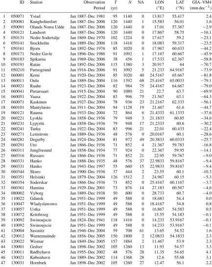
Fig. 2. Estimated trends in the 10% (blue), 50% (green) and 90% (red) sea-level quantiles from the København tide gauge, obtained using
linear and spline QR (from top to bottom: linear QR,L1-splines (linear) withλ= 0andλ >0,L∞-splines (quadratic) withλ= 0andλ >0)
obtained with (left) and without (right) removing the annual cycle from the original record. All spline models have been obtained with the
cobs99package inRusing an automatic parameter selection forλbased onAIC.
for neighbouring quantiles (Fig. 3). This results from the automatic selection of the number of active knots and the re-sulting smoothing parameterλ, which is carried out indepen-dently for eachαhere. Specifically, in typical optimisation problems, there are multiple very similar optima (in terms of the associatedAICvalues) which seem to be taken here for different quantiles. In fact, both the extreme quantiles and these “outliers” have the strongest variability, which is ex-pressed by the highest standard errors for the mean monthly increments (SE( ¯β) =σβ/
√
nwithβ¯andσβbeing the mean
value and standard deviations of monthly increments of the estimated quantile functions). If we use a fixed value ofλfor all quantilesα, this effect vanishes (see Sect. 4.3).
The obtained results underline that local sea-level trends are hardly uniform, but characterised by temporary increases
as well as decreases in slope. This holds for trends in mean and median as well as for those in arbitrary quantiles. The temporal changes in slope could originate from long-term variations in other covariates, particularly meteorological pa-rameters such as air temperature, pressure, or solar irradia-tion. We will briefly come back to such effects in the fur-ther course of this paper when studying temporal variations in long-term sea-level trends in some more detail. However, a detailed discussion of the possible co-evolution of meteo-rological observables and RSL (H¨unicke and Zorita, 2006) is beyond the scope of the present work and will remain a subject of future research. Besides these limitations of the present study, we emphasise that a detailed investigation of the robustness of the estimated nonparametric trend func-tions and the identification of possible periods with
acceler-Fig. 2. Estimated trends in the 10 % (blue), 50 % (green) and 90 % (red) sea-level quantiles from the København tide gauge, obtained using
linear and spline QR (from top to bottom: linear QR,L1-splines (linear) withλ=0 andλ >0,L∞-splines (quadratic) withλ=0 andλ >0) obtained with (left) and without (right) removing the annual cycle from the original record. All spline models have been obtained with the
cobs99package inRusing an automatic parameter selection forλbased on AIC.
lower, and larger slopes for higher quantiles. As in a previous study (Barbosa, 2008), this appears to be a generic feature of monthly tide gauge records from the Baltic Sea.
Careful inspection of the average quantile slopes obtained with different variants of spline QR reveals that the trends in-fered by nonparametric QR are qualitatively consistent with those shown by linear QR. There are, however, some dis-tinct exceptions: On the one hand, there is a clear tendency for the extreme high and low quantiles estimated in a non-parametric way not to fall into the confidence bounds of the linear model. We relate this to the fact that for properly es-timating extreme quantiles (e.g. below 5 % and above 95 %), a very high number of data is required, which is not avail-able in the case of monthly records. On the other hand, there are distinct outliers for the spline-based methods where the
estimated mean slopes differ strongly from those obtained for neighbouring quantiles (Fig. 3). This results from the automatic selection of the number of active knots and the re-sulting smoothing parameterλ, which is carried out indepen-dently for eachαhere. Specifically, in typical optimisation problems, there are multiple very similar optima (in terms of the associated AIC values) which seem to be taken here for different quantiles. In fact, both the extreme quantiles and these “outliers” have the strongest variability, which is ex-pressed by the highest standard errors for the mean monthly increments (SE(β)¯ =σ
β/
√
nwithβ¯andσ
β being the mean
102 R. V. Donner et al.: Linear and nonparametric long-term trends in Baltic sea-level variability 8 R.V. Donner et al.: Spatial patterns of linear and nonparametric long-term trends in Baltic sea-level variability
0.0 0.2 0.4 0.6 0.8 1.0
−15
01
0
slopes(mm/dec)
0.0 0.2 0.4 0.6 0.8 1.0
−15
01
0
0.0 0.2 0.4 0.6 0.8 1.0
−15
01
0
slopes(mm/dec)
0.0 0.2 0.4 0.6 0.8 1.0
−15
01
0
0.0 0.2 0.4 0.6 0.8 1.0
−15
01
0
slopes(mm/dec)
0.0 0.2 0.4 0.6 0.8 1.0
−15
01
0
0.0 0.2 0.4 0.6 0.8 1.0
−15
01
0
slopes(mm/dec)
0.0 0.2 0.4 0.6 0.8 1.0
−15
01
0
0.0 0.2 0.4 0.6 0.8 1.0
−15
01
0
slopes(mm/dec)
0.0 0.2 0.4 0.6 0.8 1.0
−15
01
0
Annual cycle removed
Linear QR
L
1-splines with λ=0
L
1-splines with λ>0
L
∞-splines with λ=0
L
∞-splines with λ>0
Raw data
α α
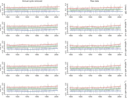
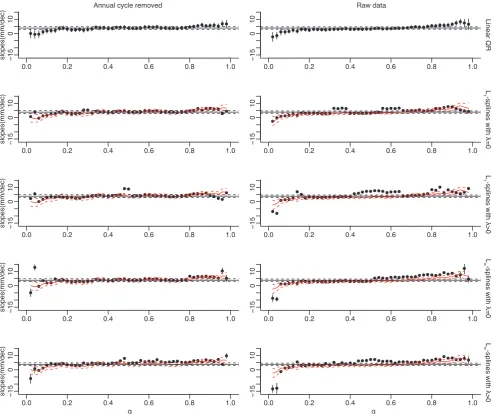
Fig. 3. Average slopesβ¯α of the estimated quantile functions for the København tide gauge, obtained using linear and spline QR (from
top to bottom: linear QR,L1-splines (linear) withλ= 0andλ >0,L∞-splines (quadratic) withλ= 0andλ >0) obtained with (left) and
without (right) removing the annual cycle from the original record. All spline models have been obtained with thecobs99package inR
using an automatic parameter selection forλbased onAIC. Error bars indicate confidence intervals corresponding to±1standard errors
of the respective linear slope estimatesβα(for linear QR models) and of the mean monthly incrementsβ¯α(for the nonparametric quantile
estimates), respectively. For the nonparametric average quantile trends, the confidence intervals for linear QR estimates are additionally shown as red lines for comparison. Horizontal lines indicate the linear trend obtained for mean sea-level (solid line, estimated using ordinary
least-squares regression) and the corresponding±1standard error confidence intervals (dashed lines).
ating or decelerating sea-level trends is necessary in order to derive insights into the complex interplay between triggering factors and sea-level response at a local scale.
In addition to the differences between different methods, Figs. 2 and 3 also allow evaluating the impact of deseason-ing on the results of QR. While details in the quantile trends indeed change qualitatively when removing the annual com-ponent from the monthly tide gauge records, it can be seen that the general trend pattern persists. Specifically, the
quan-titative differences between the mean trends in lower and up-per quantiles are a robust feature that is not altered by the corresponding preprocessing. Hence, as long as one is in-terested in the average long-term trends only, deseasoning of monthly tide gauge records is not necessary. In turn, if one is interested in temporal changes in the trends (in particular, the acceleration or deceleration of sea-level rise at a given site), the annual component plays a considerable role as it signif-icantly interferes with the trend on annual to decadal
time-Fig. 3. Average slopesβ¯
α of the estimated quantile functions for the København tide gauge, obtained using linear and spline QR (from
top to bottom: linear QR,L1-splines (linear) withλ=0 andλ >0,L∞-splines (quadratic) withλ=0 andλ >0) obtained with (left) and without (right) removing the annual cycle from the original record. All spline models have been estimated with thecobs99package in
Rusing an automatic parameter selection forλbased on AIC. Error bars indicate confidence intervals corresponding to±1 standard errors of the respective linear slope estimatesβα (for linear QR models) and of the mean monthly incrementsβ¯α(for the nonparametric quantile
estimates), respectively. For the nonparametric average quantile trends, the confidence intervals for linear QR estimates are additionally shown as red lines for comparison. Horizontal lines indicate the linear trend obtained for mean sea-level (solid line, estimated using ordinary least-squares regression) and the corresponding±1 standard error confidence intervals (dashed lines).
The obtained results underline that local sea-level trends are hardly uniform, but characterised by temporary increases as well as decreases in slope. This holds for trends in mean and median as well as for those in arbitrary quantiles. The temporal changes in slope could originate from long-term variations in other covariates, particularly meteorological pa-rameters such as air temperature, pressure, or solar irradia-tion. We will briefly come back to such effects in the fur-ther course of this paper when studying temporal variations
R. V. Donner et al.: Linear and nonparametric long-term trends in Baltic sea-level variability 103
derive insights into the complex interplay between triggering factors and sea-level response at a local scale.
In addition to the differences between different methods, Figs. 2 and 3 also allow evaluating the impact of deseason-ing on the results of QR. While details in the quantile trends indeed change qualitatively when removing the annual com-ponent from the monthly tide gauge records, it can be seen that the general trend pattern persists. Specifically, the quan-titative differences between the mean trends in lower and up-per quantiles are a robust feature that is not altered by the corresponding preprocessing. Hence, as long as one is in-terested in the average long-term trends only, deseasoning of monthly tide gauge records is not necessary. In turn, if one is interested in temporal changes in the trends (in particular, the acceleration or deceleration of sea-level rise at a given site), the annual component plays a considerable role as it signif-icantly interferes with the trend on annual to decadal time-scales. This calls for a careful treatment of the annual cycle depending on the specific research question under study. 4.2 Spatial patterns of linear quantile trends
Previous research on Baltic sea-level variability from tide gauge data has mainly focussed on the consideration of in-dividual tide gauges (Barbosa, 2008). Given the complete amount of records provided by PSMSL, in this work we are able to study the underlying spatial patterns of long-term sea-level trends. A first insight is gained by an inspection of lin-ear quantile trends obtained for all 47 available tide gauges. Note that although only data from the period 1898–2002 will be considered in the following, the actual time intervals cov-ered by the individual records are substantially different (see Table 1).
In general, the trends of RSL in the Baltic area derived from QR include both changes due to vertical land move-ments as well as changes in the height of the sea surface itself. In order to separate both effects, Fig. 4a–c shows the results of linear QR corrected for the influence of land movements by subtracting the trend from the GIA model. A spatially-consistent pattern is found for the low and high quantiles (α=0.1 and 0.9, respectively) as well as the me-dian, with positive slopes in the southern area, negative slopes in the Gulf of Finland and Bothnian Sea, and posi-tive slopes in the northernmost stations in the Bothnian Bay. Especially large positive trends are found along the Polish coast, whereas the results obtained for the south-western part of the Baltic Sea (Germany, Denmark, southern Sweden) show a slower rate of increase. On the one hand, these find-ings could just result from the different time coverage of the individual tide gauge records. In particular, the available data from Poland cover only the time period starting in 1951 (i.e. the most recent decades), whereas many of the other records contain measurements from considerably earlier times. This would have a significant effect especially if the trends in RSL quantiles are not constant in time. We will explicitly
study the influence of a homogenous reference period on the obtained spatial trend patterns below, whereas the particu-lar question of possibly changing trends will be further ad-dresses in Sect. 4.5. On the other hand, the spatial pattern could also result from uncertain estimates of the postglacial rebound rates in the considered GIA model. However, the information available to us does not allow further evaluating this possibility in this work.
The major conceptual advantage of QR in comparison with conventional methods of trend analysis for the mean is its ability to provide information on changes of the entire probability distribution of RSL. In order to highlight the dif-ferences, Fig. 4d–f shows the residual quantile trends relative to the corresponding trend in mean sea-level. For the 10 % quantile most slopes are consistently, but only very weakly negative, indicating that the trend in lower RSL quantiles due to global sea-level rise is somewhat less positive than the trend in the mean. For the 90 % quantile the slopes are positive in most of the Baltic with the exception of some tide gauges in the Archipelago Sea and the Gulf of Finland (where the associated uncertainties of the trend estimates are, however, rather large), indicating that upper RSL quantiles rise generally faster than the mean. Both observations to-gether indicate that the total variability of RSL is increasing in the entire Baltic Sea, which can be attributed to a general intensification of atmospheric dynamics forcing short-term sea-level variability.
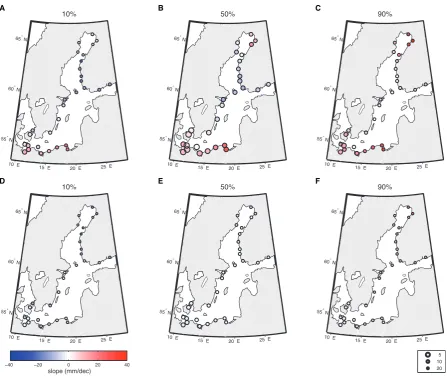
From the analysis presented so far, it has not yet been pos-sible to draw systematic conclusions due to the different pe-riods covered by the individual tide gauge records. In or-der to solve this problem, we next apply linear QR to all records completely covering the second half of the 20th cen-tury (1951–1999) without significant gaps, which are avail-able for 30 tide gauges. In this case, the observed spatial pattern becomes more coherent. For the relative sea-level trends corrected for GIA effects (Fig. 5a–c), the upper quan-tiles show consistent positive trends in the entire Baltic Sea, whereas median and lower quantiles show negative relative trends in vast parts of the study area with the exception of the southwestern Baltic Sea (Poland, Germany, Denmark, south-ern Sweden) and northsouth-ernmost Gulf of Bothnia, where also the high quantiles show the strongest positive trends. When considering the difference between the quantile slopes and the mean sea-level trend, we find consistently positive rela-tive trends in the higher quantiles and negarela-tive ones in inter-mediate (median) and lower quantiles (Fig. 5d–f) with only few local exceptions. These results are in excellent agree-ment with those obtained by Barbosa (2008) for individual stations. Note, however, that these relative quantile trends have considerably lower magnitudes and higher standard er-rors than those in comparison with the mean GIA slope.
104 R. V. Donner et al.: Linear and nonparametric long-term trends in Baltic sea-level variability 10 R.V. Donner et al.: Spatial patterns of linear and nonparametric long-term trends in Baltic sea-level variability
A B C
D E F
slope (mm/dec)
−40 −20 0 20 40
10%
10° E
15° E 20° E 25° E
55° N
60° N
65° N
50%
10° E
15° E 20° E 25° E
55° N
60° N
65° N
90%
10° E
15° E 20° E 25° E
55° N
60° N
65° N
10%
10° E
15° E 20° E 25° E
55° N
60° N
65° N
50%
10° E
15° E 20° E 25° E
55° N
60° N
65° N
90%
10° E
15° E 20° E 25° E
55° N
60° N
65° N
0.5 1.0 2.0
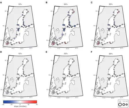
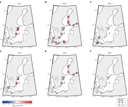
Fig. 4.Slopesβ0.1,β0.5andβ0.9of the linear trends in the (A,D) 10%, (B,E) 50% and (C,F) 90% quantiles of the 47 tide gauge records in the
time period 1898-2002 (cf. Barbosa (2008)), corrected for the overall mean trends obtained from the GIA model (A-C) and trends in mean sea-level (D-F, including contributions from global sea-level changes, but not explicitly corrected for glacial isostatic adjustment processes). Colours indicate the slope values, sizes of the associated circles their standard errors in mm/dec (large circles: low uncertainty, small circles: high uncertainty). Note that the statistical confidence of trends corrected for linear trends in the mean is smaller, since the standard errors of estimated total quantile trends and trends in the mean add up, whereas we have implicitly assumed the absence of uncertainty in the GIA model as a simplification.
4.3 Parameter selection for nonparametric QR
In order to systematically compare the results of linear QR presented above with those of a particular nonparametric QR method, a reasonable choice of the regularisation parameter
λhas to be determined. In the following, we will illustrate this choice for some exemplary tide gauges. Subsequently, in Sect. 4.4 the resulting spatial trend patterns for selected quantiles will be compared with the outcomes of linear QR.
As discussed in Sect. 3.3, there are two widely ac-cepted possibilities for determining proper values forλ, i.e., penalised-likelihood and cross-validation criteria. In case of
nonparametric quantile regression, we request the solution of the underlying estimation problem (i) to be optimal and sparse in the sense of a high fidelity and a low number of pa-rameters and (ii) not to differ “too much” from the linear QR model. The second requirement allows for moderate long-term variations in the instantaneous slope of the estimated quantile trends, but does not permit strong short-term fluctu-ations. While the first requirement is quantified by means of
AIC orSIC, the second constraint is captured by the vari-anceσ2
resof the residual nonparametric trend model with
re-spect to the linear one.
Althoughλshould be in principle selected independently
Fig. 4. Slopesβ0.1,β0.5andβ0.9of the linear trends in the (A, D) 10 %, (B, E) 50 % and (C, F) 90 % quantiles of the 47 tide gauge records in
the time period 1898–2002 (cf. Barbosa, 2008), corrected for the overall mean trends obtained from the GIA model (A–C) and trends in mean sea-level (D–F, including contributions from global sea-level changes, but not explicitly corrected for glacial isostatic adjustment processes). Colours indicate the slope values, sizes of the associated circles their standard errors in mm dec−1(large circles: low uncertainty, small circles: high uncertainty). Note that the statistical confidence of trends corrected for linear trends in the mean is smaller, since the standard errors of estimated total quantile trends and trends in the mean add up, whereas we have implicitly assumed the absence of uncertainty in the GIA model as a simplification.
intensification of zonal wind and cyclones. In general, a detailed interpretation of the results at this point would be difficult and speculative, since sea-level is influenced by a multiplicity of different variables (wind, temperature,...) that are mutually interdependent and change over time in a com-plicated way. In turn, much more detailed future studies – specifically involving information on possible triggering fac-tors as covariates – would be necessary to develop and test corresponding hypotheses.
As an intermediate summary, we conclude that (i) the quantile trends obtained from linear QR are distinctively dif-ferent from trends in the mean, and that (ii) the GIA pro-cesses cannot explain the observed changes in Baltic sea-level quantiles.
4.3 Parameter selection for nonparametric QR
In order to systematically compare the results of linear QR presented above with those of a particular nonparametric QR method, a reasonable choice of the regularisation parameter λhas to be determined. In the following, we will illustrate this choice for some exemplary tide gauges. Subsequently, in Sect. 4.4 the resulting spatial trend patterns for selected quantiles will be compared with the outcomes of linear QR.
R. V. Donner et al.: Linear and nonparametric long-term trends in Baltic sea-level variability 105 R.V. Donner et al.: Spatial patterns of linear and nonparametric long-term trends in Baltic sea-level variability 11
A B C
D E F
10%
10° E
15° E 20° E 25° E
55° N
60° N
65° N
50%
10° E
15° E 20° E 25° E
55° N
60° N
65° N
90%
10° E
15° E 20° E 25° E
55° N
60° N
65° N
10%
10° E
15° E 20° E 25° E
55° N
60° N
65° N
50%
10° E
15° E 20° E 25° E
55° N
60° N
65° N
slope (mm/dec)
−40 −20 0 20 40
90%
10° E
15° E 20° E 25° E
55° N
60° N
65° N
5 10 20
Fig. 5.As in Fig. 4 for the 30 available tide gauge records for the time period 1951-1999.
for each quantileα, an automatic parametric selection based on the optimisation of some individual criterion can lead to inconsistencies between the mean slopes obtained for differ-ent quantiles (cf. Sect. 4.1). As a consequence, we search for a reasonable trade-off between optimising AIC and keep-ing the deviations from the linear trend model in an accept-able range simultaneously for low, intermediate, and high quantiles. As an example, Fig. 6 shows the values ofAIC
andσres in dependence onλ for the10%,50%, and 90%
quantiles estimated withL1-smoothing splines (using theR
packagequantreg) for three Danish tide gauges (Gedser, København, and Hornbæk). The grey bars highlight values of
λfor which both requirements of highAICand low residual variance are still fulfilled for all three considered quantiles (these criteria obviously remain valid for higher values ofλ
as well, however, we are seeking for a solution that allows for a maximum degree of variability with a still reasonable smoothness). From these three examples, we conclude that a
value ofλ= 4is a reasonable choice for the following anal-yses.
4.4 Spatial patterns of nonparametric quantile trends
In order to understand the potential influence of nonlinear-ities in the quantile trends, the 30 selected stations previ-ously analysed by means of linear QR have been subjected to an additional nonparametric QR usingL1-smoothing splines
with a fixedλ= 4for all considered quantiles (see above).
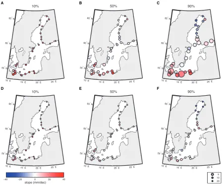
In Fig. 7, the average slopes of the nonparametric quantile trends taken over the entire period of observation are shown. From a conceptual perspective, using average quantile trends in situations when the actual changes of the probability distri-bution functions depend on both the considered quantile and time obviously leads to a loss of information. Even more, the possibility to interpret average trends in a meaningful way clearly depends on the temporary variations of the instan-Fig. 5. As in instan-Fig. 4 for the 30 available tide gauge records for the time period 1951–1999.
sparse in the sense of a high fidelity and a low number of pa-rameters and (ii) not to differ “too much” from the linear QR model. The second requirement allows for moderate long-term variations in the instantaneous slope of the estimated quantile trends, but does not permit strong short-term fluctu-ations. While the first requirement is quantified by means of AIC or SIC, the second constraint is captured by the variance σres2 of the residual nonparametric trend model with respect to the linear one.
Althoughλshould be in principle selected independently for each quantileα, an automatic parametric selection based on the optimisation of some individual criterion can lead to inconsistencies between the mean slopes obtained for differ-ent quantiles (cf. Sect. 4.1). As a consequence, we search for a reasonable trade-off between optimising AIC and keep-ing the deviations from the linear trend model in an accept-able range simultaneously for low, intermediate, and high quantiles. As an example, Fig. 6 shows the values of AIC andσres in dependence on λfor the 10 %, 50 %, and 90 %
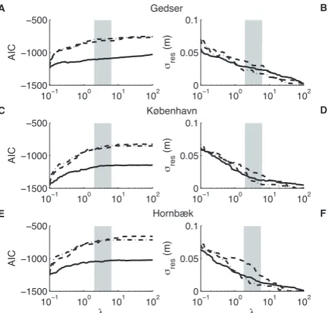
quantiles estimated withL1-smoothing splines (using theR packagequantreg) for three Danish tide gauges (Gedser, København, and Hornbæk). The grey bars highlight values of λfor which both requirements of high AIC and low residual variance are still fulfilled for all three considered quantiles (these criteria obviously remain valid for higher values ofλ as well, however, we are seeking for a solution that allows for a maximum degree of variability with a still reasonable smoothness). From these three examples, we conclude that a value ofλ=4 is a reasonable choice for the following anal-yses.
4.4 Spatial patterns of nonparametric quantile trends
106 R. V. Donner et al.: Linear and nonparametric long-term trends in Baltic sea-level variability 12 R.V. Donner et al.: Spatial patterns of linear and nonparametric long-term trends in Baltic sea-level variability
10−1 100 101 102 −1500
−1000 −500
AIC
100−1 100 101 102 0.05
0.1
σres
(m)
10−1 100 101 102 −1500
−1000 −500
AIC
100−1 100 101 102 0.05
0.1
σres
(m)
10−1 100 101 102 −1500
−1000 −500
λ
AIC
100−1 100 101 102 0.05 0.1 λ σres (m) A C E B D F Gedser København Hornbæk
Fig. 6.Dependence of theAICcriterion (left panels) and the resid-ual standard deviationsσreswith respect to the corresponding
lin-ear quantile models (right panels) on the smoothing parameter λ for the 10% (dashed), 50% (solid), and 90% (dash-dotted) quantile functions obtained for three example records from Denmark (time period 1951-1999) usingL1-smoothing (piecewise linear) splines. A reasonable choice forλis obtained whereAICandσresstart to
significantly decrease and increase, respectively (indicated by grey bars).
taneous trends. For this purpose, information on the latter aspect is encoded in Fig. 7 in terms of different symbol sizes.
Comparing the average slopes of the nonparametric trends with the linear quantile trends (Fig. 5), distinct differences are observed. Specifically, for the sea surface heights cor-rected for GIA, we find consistent positive trends in the southern Baltic Sea and the Gulf of Finland for all quan-tiles. In the central part of the Baltic Sea as well as most tide gauges in the Gulf of Bothnia, the relative trends with respect to the GIA model are positive for lower quantiles, but become negative for higher quantiles in the northern Gulf of Bothnia. Differences between linear and spline model are mainly found in the lower quantiles, where we observe neg-ative trends along the Swedish and Finnish coastlines for the linear, but positive ones for the spline estimates. We have to emphasise, however, that especially for quantiles deviat-ing strongly from the median, the results obtained with the spline model show a considerable degree of sensitivity with respect to changes at both ends of the considered time se-ries, e.g., the observed average quantile trends can change strongly if the records are extended by another year or so. This is due to the generally strong effect of boundary con-ditions on splines (Rice and Rosenblatt, 1983), which does
more extreme quantiles, since they are statistically less well determined.
Taking the trends in mean sea-level instead of the mean GIA rates as a basis, the overall spatial pattern does not change qualitatively. Specifically, when comparing aver-age trends from the spline model with the linear quantile trends, all results become more pronounced underlining the importance of the nonlinear characteristics for studying low-frequency sea-level variability in the Baltic Sea. In general, we have to note that the absolute differences between linear andmean nonparametric trends are not statistically signifi-cant when considering the standard errors of the estimates.
With respect to the results discussed above, we empha-sise that we have only studied the behaviour ofL1-smoothing
splines. From the present analysis, it cannot be ruled out that L∞-smoothing splines could display a somewhat different
spatial pattern for selected quantiles. A detailed comparison of different approaches is beyond the scope of the present study, but should be performed in future work. In general, we note that estimating nonparametric quantile models is computationally more demanding than linear QR, which is reflected in the corresponding CPU times required for per-forming our analyses. With respect to the different algo-rithms used for spline QR, the algorithm implemented in the
cobs99package is somewhat more efficient than that used
in thequantregpackage when run on the same hard- and software environment.
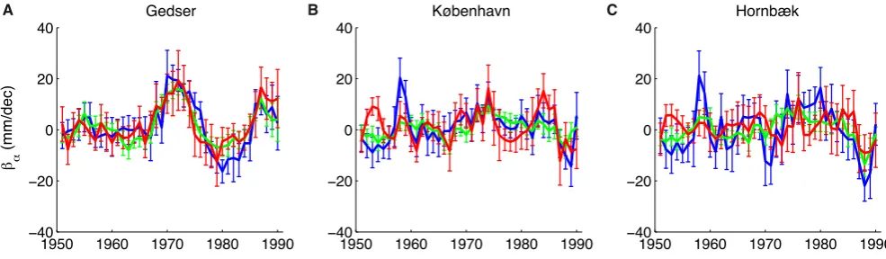
4.5 Acceleration of local sea-level trends
The possible acceleration of global sea-level rise has recently attracted considerable interest (Woodworth, 1990; Douglas, 1992; Church and White, 2006; Jevrejeva et al., 2008; Wood-worth et al., 2009; Merrifield et al., 2009; Houston and Dean, 2011; Rahmstorf and Vermeer, 2011). In order to comple-ment our previous analysis, in the following, we study pos-sible evidence for changes in sea-level quantile trends on the local scale. For this purpose, we estimate linear mod-els for the quantile trends for running windows of width 10 years (Holgate, 2007) with a mutual offset of 1 year. To as-sure comparability of our results, we again restrict our atten-tion to the 30 tide gauge records that cover the time period 1951-1999 completely, yielding in total 40 linear trend val-ues for each record. As examples, the temporal variability of local linear quantile trends for the three Danish tide gauges from Fig. 6 is shown in Fig. 8. The observed temporal vari-ability of the obtained trends shows significant changes that are different even for these spatially close locations. At the Gedser tide gauge (Fig. 8A) there is a marked multi-decadal variability that is common to all three considered quantiles. København and Hornbæk also display decadal-scale changes in trends, though less pronounced, and a similar qualita-tive behaviour, particularly for the lower quantiles. A de-tailed analysis of these features and possible interpretations
Fig. 6. Dependence of the AIC criterion (left panels) and the
resid-ual standard deviationsσreswith respect to the corresponding linear quantile models (right panels) on the smoothing parameterλfor the 10 % (dashed), 50 % (solid), and 90 % (dash-dotted) quantile functions obtained for three example records from Denmark (time period 1951–1999) usingL1-smoothing (piecewise linear) splines. We propose that a reasonable reasonable choice forλis obtained where AIC andσresstart to significantly decrease and increase, re-spectively (indicated by grey bars).
trends taken over the entire period of observation are shown. From a conceptual perspective, using average quantile trends in situations when the actual changes of the probability distri-bution functions depend on both the considered quantile and time obviously leads to a loss of information. Even more, the possibility to interpret average trends in a meaningful way clearly depends on the temporary variations of the instan-taneous trends. For this purpose, information on the latter aspect is encoded in Fig. 7 in terms of different symbol sizes. Comparing the average slopes of the nonparametric trends with the linear quantile trends (Fig. 5), distinct differences are observed. Specifically, for the sea surface heights cor-rected for GIA, we find consistent positive trends in the southern Baltic Sea and the Gulf of Finland for all quan-tiles. In the central part of the Baltic Sea as well as most tide gauges in the Gulf of Bothnia, the relative trends with respect to the GIA model are positive for lower quantiles, but become negative for higher quantiles in the northern Gulf of Bothnia. Differences between linear and spline model are mainly found in the lower quantiles, where we observe neg-ative trends along the Swedish and Finnish coastlines for the linear, but positive ones for the spline estimates. We have to emphasise, however, that especially for quantiles deviat-ing strongly from the median, the results obtained with the
spline model show a considerable degree of sensitivity with respect to changes at both ends of the considered time series, e.g. the observed average quantile trends can change strongly if the records are extended by another year or so. This is due to the generally strong effect of boundary conditions on splines (Rice and Rosenblatt, 1983), which does not apply to linear spline models and is more severe for the more extreme quantiles, since they are statistically less well determined.
Taking the trends in mean sea-level instead of the mean GIA rates as a basis, the overall spatial pattern does not change qualitatively. Specifically, when comparing aver-age trends from the spline model with the linear quantile trends, all results become more pronounced underlining the importance of the nonlinear characteristics for studying low-frequency sea-level variability in the Baltic Sea. In general, we have to note that the absolute differences between linear and mean nonparametric trends are not statistically signifi-cant when considering the standard errors of the estimates.
With respect to the results discussed above, we empha-sise that we have only studied the behaviour ofL1-smoothing splines. From the present analysis, it cannot be ruled out that L∞-smoothing splines could display a somewhat different
spatial pattern for selected quantiles. A detailed comparison of different approaches is beyond the scope of the present study, but should be performed in future work. In general, we note that estimating nonparametric quantile models is computationally more demanding than linear QR, which is reflected in the corresponding CPU times required for per-forming our analyses. With respect to the different algo-rithms used for spline QR, the algorithm implemented in the
cobs99package is somewhat more efficient than that used in thequantregpackage when run on the same hard- and software environment.
4.5 Acceleration of local sea-level trends
The possible acceleration of global sea-level rise has recently attracted considerable interest (Woodworth, 1990; Douglas, 1992; Church and White, 2006; Jevrejeva et al., 2008; Wood-worth et al., 2009; Merrifield et al., 2009; Houston and Dean, 2011; Rahmstorf and Vermeer, 2011). In order to comple-ment our previous analysis, in the following, we study pos-sible evidence for changes in sea-level quantile trends on the local scale. For this purpose, we estimate linear mod-els for the quantile trends for running windows of width 10 years (Holgate, 2007) with a mutual offset of 1 yr. To assure comparability of our results, we again restrict our attention to the 30 tide gauge records that cover the time period 1951– 1999 completely, yielding in total 40 linear trend values for each record. As examples, the temporal variability of local linear quantile trends for the three Danish tide gauges from Fig. 6 is shown in Fig. 8.