Particle trajectories beneath wave-current interaction in a two-dimensional field

www.nonlin-processes-geophys.net/19/185/2012/ doi:10.5194/npg-19-185-2012

© Author(s) 2012. CC Attribution 3.0 License.

Nonlinear Processes

in Geophysics

Particle trajectories beneath wave-current interaction in a

two-dimensional field

Y.-Y. Chen1, 3, H.-C. Hsu2, and H.-H. Hwung3

1_{Dept. of Marine Environment and Eng., National Sun Yat-Sen Univ., Kaohsiung 804, Taiwan} 2_{Tainan Hydraulics Laboratory, National Cheng Kung Univ., Tainan 701, Taiwan}

3_{Dept. of Hydraulic and Ocean Eng., National Cheng Kung Univ., Tainan 701, Taiwan} Correspondence to: H.-C. Hsu ([email protected])

Received: 25 October 2011 – Revised: 29 January 2012 – Accepted: 6 February 2012 – Published: 16 March 2012

Abstract. Within the Lagrangian reference framework we present a third-order trajectory solution for water particles in a two-dimensional wave-current interaction flow. The ex-plicit parametric solution highlights the trajectory of a wa-ter particle and the wave kinematics above the mean wawa-ter level and within a vertical water column, which were calcu-lated previously by an approximation method using an Eu-lerian approach. Mass transport associated with a particle displacement can now be obtained directly in Lagrangian form without using the transformation from Eulerian to La-grangian coordinates. In particular, the LaLa-grangian wave fre-quency and the Lagrangian mean level of particle motion can also be obtained, which are different from those in an Eule-rian description. A series of laboratory experiments are per-formed to measure the trajectories of particles. By compar-ing the present asymptotic solution with laboratory experi-ments data, it is found that theoretical results show excellent agreement with experimental data. Moreover, the influence of a following current is found to increase the relative hor-izontal distance traveled by a water particle, while the con-verse is true in the case of an opposing current.

1 Introduction

The problem of nonlinear water waves propagating through areas containing tidal, ocean or discharge current is an im-portant issue in marine environments. The interaction be-tween these flows plays vital roles in many aspect of coastal and ocean engineering, for example forces due to such flow fields on fixed or floating offshore wind turbines, sediment transport, contaminant and nutrient dispersion. The phe-nomenon of wave-current interaction has been studied ex-tensively since the 1970s. Several theoretical solutions for waves on currents with uniform or sheared profiles have been

well documented in the review articles of Peregrine (1976), Jonsson (1990) and Thomas and Klopman (1997). Reports are also available on experimental studies for combined wave and current covering various aspects of this problem (Bre-vik, 1980; Constantin and Strauss, 2004; Kemp and Simons, 1982, 1988; Thomas, 1981, 1990).

Most previous theories dealing with wave-current interac-tions have employed the Eulerian description, in which the free surface fluctuations can be expressed in a Taylor series expansion relative to a fixed water level (i.e., the still water level). This implicitly assumes that the surface profile of a wave is a differentiable single-valued function. Unlike the Eulerian free surface, which is given as an implicit function, a Lagrangian surface is described through a parametric repre-sentation of the position of a particle. The use of Lagrangian coordinates yields the only known nontrivial exact solutions to the governing equations for gravity water waves (i.e., Ger-stner’s solution for deep-water waves (Gerstner, 1802) and a recently found edge wave solution along a sloping beach (Constantin, 2001) which was extended to stratified flows (R. Stuhlmeier, 2012)). The main advantage of such a de-scription is to allow better flexibility for describing the actual shape of the ocean surface, which will be demonstrated later in this paper. Based on this reason, it has been shown that the Lagrangian description is more appropriate for the motion of the limiting free surface, which cannot be captured by the classical Eulerian solutions (Biesel, 1952; Chen et al., 2006; Naciri and Mei, 1992). However, reports on this notable im-provement using Lagrangian description are rather limited.

deep water waves in the Lagrangian formulae and ob-tained the first-order Lagrangian solution. Sanderson (1985) obtained second-order solutions for small amplitude inter-nal waves in a Lagrangian coordinate system. Ng (2004) re-examined the problem of mass transport due to partial standing waves in one and two layer fluids. Buldakov et al. (2006) developed a Lagrangian asymptotic formulation up to the fifth order for nonlinear water waves in deep water. Clamond (2007) obtained a third-order Lagrangian solution for gravity waves in finite-depth water and a seventh-order solution for deep water waves. To date, only a limited few theoretical solutions are derived for wave-current interaction in Lagrangian coordinates. Umeyama (2010) gave a wrong third-order solution of particle trajectory, which did not in-clude Lagrangian wave frequency and Lagrangian mean level shown in Eqs. (88) and (90) derived in this paper. Zaman and Baddour (2010) presented a first-order solution of particle trajectory in the combined wave-current flow. The theoretical investigations of the particle paths beneath a Stokes wave and solitary wave were recently undertaken by Constantin (2006, 2010).

This paper aims to study particle trajectories of a two-dimensional wave-current field based on the fully Lagrangian framework, and to derive asymptotic solutions that can be used to describe the dynamics for the entire flow field. Pre-vious works on progressive, standing, short-crested gravity waves and gravity-capillary waves have been summarized in the papers by Chen and Hsu (2009), Chen et al. (2010) and Hsu et al. (2010). In this paper, we look into the ef-fect of uniform current on a gravity water wave, the motion of which is assumed to be inviscid, incompressible and ir-rotational. A set of governing equations in Lagrangian co-ordinates is derived for two-dimensional progressive gravity waves on uniform current in a constant water depth. We will construct asymptotic expansions of the solution in powers of the wave amplitude, which is assumed to be small using the Lindstedt-Poincare perturbation method. Approximate solu-tions including particle trajectory, Lagrangian wave period, the Lagrangian mean level and mass transport velocity are derived up to the third order. A detailed analysis of influ-ences of the uniform current is then carried out. Finally, to validate the accuracy of the analytical results, a series of lab-oratory experiments are performed. The trajectories of water particles in a wave-current interaction flow are shown to have an excellent agreement with experimental data.

The problem formulation and the procedures for construct-ing asymptotic solutions are described in Sect. 2. In Sect. 3, we derive equations for the properties of surface-particle tra-jectories and present results for some selected wave-current flow. Section 4 is devoted to a description of experimental apparatus and of the experimental procedure. In Sect. 5 the trajectories of surface and subsurface particles are presented. Some concluding remarks are given in the final section.

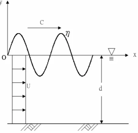
Figure 1 Definition sketch showing a system of progressive wave train on a uniform

current.

Fig. 1. Definition sketch showing a system of progressive wave train on a uniform current.

2 Formulation of the problem

We consider the problem of a two-dimensional monochro-matic wave with a steady uniform current on an imperme-able and horizontal bed (Fig. 1). The fluid motion is taken to be two-dimensional and irrotational, and the wave is right-going. We choose Cartesian axes withx pointing horizon-tally to the right andyvertically upward from the still water level. The mathematical problem is formulated in terms of Lagrangian variables,aandb,which define the original po-sition of individual fluid particles. At any timet, we letb=0 be the free surface, andb=d be the bottom. The Carte-sian coordinates (x(a,b,t ),y(a,b,t )) of fluid particles and the fluid pressurep(a,b,t )are the unknowns. Based on the Lagrangian description, the governing equations and bound-ary conditions for two-dimensional irrotational free-surface flow are summarized as follows:

J=∂(x,y)

∂(a,b)=1, (1)

∂J

∂t =xatyb+xaybt−xbtya−xbyat=0, (2)

xatxb−xbtxa+yatyb−ybtya=0, (3)

∂φ

∂a=xtxa+ytya, ∂φ

∂b=xtxb+ytyb, (4)

p

ρ = −

∂φ

∂t −gy+

1 2[(

∂x ∂t)

2₊₍∂y

∂t)

2_{], (5)}

v=yt=0, y=b= −d. (7)

In Eqs. (1)–(7), subscriptsa,b, andt denote partial deriva-tives with respect to the specified variables,U denotes the speed of a steady uniform current, g is the gravitational acceleration, p(a,b,t )is water pressure, φ (a,b,t ) is a ve-locity potential function in the Lagrangian system. Except for Eqs. (4) and (5), the fundamental physical relationships defining the equations above have been derived previously (Lamb, 1932; Naciri and Mei, 1992). Equation (1) is the con-tinuity equation based on the invariant condition on the vol-ume of a Lagrangian particle; Eq. (2) is the differentiation of Eq. (1) with respect to time. Equations (3) and (4) denote the irrotational flow condition and the corresponding Lagrangian velocity potential, respectively. Equation (5) is the Bernoulli equation for the irrotational flow in the Lagrangian descrip-tion. The wave motion has to satisfy a number of boundary conditions at the bottom and on the free water surface. Equa-tion (6) is the dynamic boundary condiEqua-tion of zero pressure at the free surface. On a rigid and impermeable bottom, the no-flux bottom boundary condition gives Eq. (7).

3 Asymptotic solutions

To solve the nonlinear Eqs. (1)–(7), we introduce the La-grangian angular frequencyσ of particle motion, which is a function of a nonlinear parameter and the Lagrangian level label(b), making the wave periodic in timetand spacex(or

a)in order to avoid a secular term. We use the Lindstedt-Poincare technique that yields uniform expansions to un-cover the solutions in the Lagrangian system. The issue of convergence is covered by the recent regularity results in Constantin and Esher (2011). In the Lagrangian approach, the particle positionsx andy, the potential function φ, and pressurep are considered as functions of independent vari-ablesa,band timet. Following Chen and Hsu (2009), Chen et al. (2010) and Hsu et al. (2010), these solutions are sought in perturbation series by introducing an ordering parameter

ε, which is inserted to identify the order of the associated term:

x=a+U t+ ∞ X

n=1

εn[fn(a,b,σ t )+fn0(a,b,σ0t )], (8)

y=b+

∞ X

n=1

εn[gn(a,b,σ t )+gn0(a,b,σ0t )], (9)

φ=U a+1

2U

2_t+

∞ X

n=1

εn[φn(a,b,σ t )+φ0n(a,b,σ0t )], (10)

p= −ρgb+

∞ X

n=1

εnpn(a,b,σ t ), (11)

σ=σ0(a,b)+

∞ X

n=1

εnσn(a,b)=2πTL, (12)

where the Lagrangian variables (a,b)are defined as the two characteristic parameters. In these expressions, fn,gn, φn

andpnare expected to be associated with thenth-order

har-monic solutions. f_n0,g_n0 andφ0_n are non-periodic functions that increase linearly with time. σ=2π

TL is the angular

frequency of particle motion or the Lagrangian angular fre-quency for a particle reappearing at the same elevation. TL

is the corresponding period of particle motion. Upon substi-tuting Eqs. (8)–(12) into Eqs. (1)–(7) and collecting terms of equal order, we obtain a sequence of nonhomogeneous gov-erning equations that can be solved successively, as shown in the following sections.

3.1 First-order approximation

Collecting terms of orderε, the governing equations and the boundary conditions can be obtained as follows:

f1a+f_1a0 +g1b+g_1b0 + [σ0a(f1σ t+f_1σ0 _0t)

+σ0b(g1σ t+g1σ0 0t)]t=0,

(13)

σ0(f1aσ t+f₁0aσ0t+g1bσ t+g

0 1bσ0t)

+σ0a(f1σ t+f₁0_σ

0t)+σ0b(g1σ t+g

0 1σ0t)

+σ0{σ0a[f1(σ t )2+f0 1(σ0t )2

] +σ0b[g1(σ t )2+g0 1(σ0t )2

]}t=0,

(14)

σ0(f1bσ t+f₁0_bσ

0t−g1aσ t−g

0 1aσ0t)

+σ0b(f1σ t+f₁0σ0t)−σ0a(g1σ t+g

0 1σ0t)

+σ0{σ0b[f1(σ t )2+f0

1(σ0t )2] −σ0a[g1(σ t )2+g

0

1(σ0t )2]}t=0,

(15)

φ1a+φ10a+σ0a(φ1σ t+φ10σ0t)t

=U· [(f1a+f10a)+σ0a(f1σ t+f10σ0t)t] +σ0(f1σ t+f 0

1σ0t),

(16)

φ1b+φ10b+σ0b(φ1σ t+φ10σ0t)t

=U· [(f1b+f10b)+σ0b(f1σ t+f10σ0t)t] +σ0(g1σ t+g 0

1σ0t),

(17) p1

ρ =U·σ0(f1σ t+f

0

1σ0t)−σ0(φ1σ t+φ 0

1σ0t)−g(g1+g 0

1), (18)

p1=0 at b=0, (19)

g1σ t=g1σ0 0t=0 on b= −d. (20)

The flow is assumed periodic with a crest ata=0 andt=0, and hence the first-order solution can be easily written as

f1= −α

coshk(b+d)

coshkd sin(ka−σ t ), (21a)

g1=α

sinhk(b+d)

coshkd cos(ka−σ t ), (21b)

f₁0=g0₁=0, (21c)

σ0a=σ0b=0, (21d)

φ1=(

σ0

k −U )α

coshk(b+d)

coshkd sin(ka−σ t ), (21e)

p1

ρ = −gα

sinhkb

cosh2kdcos(ka

−σ t ), (21g)

where the parameterαrepresents the amplitude function of the particle displacement; the wave amplitude is, as usual, taken asa0=αtanhkd, wherekis the wave number (=2π/L,

Lis wave length).φ1(a,b,t )is the first-order Lagrangian

ve-locity potential andp1(a,b,t )is the first-order wave dynamic

pressure in the Lagrangian form with pressurep1=0 at the

free surfaceb= 0. Equations (21a–g) satisfy all the hydrody-namic equations formulated in Lagrangian terms including the irrotational condition, and differ from Gerstner’s wave in infinite water depth, which possesses finite vorticity. The dis-persion relation shows that the first-order Lagrangian wave frequency (σ0)is the same as that of the first-order Stokes

wave frequency in the Eulerian approach (Biesel, 1952). The first-order free surface in Lagrangian coordinates is given by settingb=0 in Eqs. (21a) and (21b), and is similar to expres-sions for the profile found from the first-order Eulerian equa-tions. Equation (21d) is the basic velocity potential solution with a steady uniform current. In Eq. (21f),σ0is the

essen-tial Lagrangian wave frequency for water particles relative to the uniform current. From this, it can be demonstrated that the Doppler’s effect is not apparent in the Lagrangian disper-sion relation. This is correct: in Eulerian frame of reference,

intrinsic wave frequencyσ0is different from absolute wave

frequency(σ0−kU ).

3.2 Second-order approximation

Collecting terms of orderε2and using Eq. (21), the govern-ing equations and the boundary conditions can be obtained as

f2a+f2a0 +g2b+g2b0 +f1ag1b−f1bg1a (22)

+(σ1af1σ t+σ1bg1σ t)t=0,

σ0(f2aσ t+f_2aσ0 _0t+g2bσ t+g0_2bσ0t)

+σ1(f1a+g1b)σ t+σ0(f1ag1b−f1bg1a)σ t

+σ1af1σ t+σ1bg1σ t+σ0[σ1af1(σ t )2+σ1bg1(σ t )2]t=0,

(23)

σ0(f2bσ t+f_2bσ0

0t−g2aσ t−g 0

2aσ0t)

+σ1(f1b−g1a)σ t+σ1bf1σ t−σ1ag1σ t

+σ0(f1af1bσ t−f1aσ tf1b+g1ag1bσ t−g1bg1aσ t)

+σ0[σ1bf1(σ t )2−σ1ag1(σ t )2]t=0,

(24)

φ2a+φ02a=U· [(f2a+f2a0 )

+σ0a(f2σ t+f2σ0 0t)t] +U·σ1atf1σ t

−σ0a(φ2σ t+φ_2σ0 0t)

+σ0(f2σ t+f_2σ0 _0t)+σ1f1σ t

+σ0(f1af1σ t+g1ag1σ t)−σ1at φ1σ t,

(25)

φ2b+φ_2b0 =U· [(f2b+f_2b0 )+σ0b(f2σ t+f_2σ0 _0t)t]

+U·σ1btf1σ t−σ0b(φ2σ t+φ0_2σ 0t)

+σ0(g2σ t+g_2σ0 _0t)+σ1g1σ t

+σ0(f1bf1σ t+g1bg1σ t)−σ1bt φ1σ t,

(26)

p2

ρ = −[σ0(φ2σ t+φ

0

2σ0t)+g(g2+g 0

2)]

−σ1φ1σ t+1₂σ₀2(f_{1σ t}2 +g_{1σ t}2 )

+U·σ0(f2σ t+f_2σ0 _0t)+U·σ1(f1σ t+f_1σ0 _0t),

(27)

and

p2=0 at b=0. (28)

g2σ t=g2σ0 0t=0 on b=−d. (29)

Substituting Eqs. (21a∼g) into Eqs. (22)–(24), the second-order governing equations in terms ofε2, including the con-tinuity equation and the irrotational condition, are given by

f2a+f_2a0 +g2b+g_2b0

=1

2k2α2· {

cosh2k(b+d) cosh2kd +

cos2(ka−σ t ) cosh2kd }

−α· {σ1a·coshk(b_coshkd+d)cos(ka−σ t )

+σ1b·sinhk(b_coshkd+d)sin(ka−σ t )} ·t,

(30)

σ0(f2aσ t+f_2aσ0 _0t+g2bσ t+g_2bσ0 _0t)

=α2·k2·σ0·sin2(ka−σ t ) cosh2kd

−α· [σ1acoshk(b_coshkd+d)cos(ka−σ t )

+σ1bsinhk(b_coshkd+d)sin(ka−σ t )]

−α·σ0· [σ1acoshk(b_coshkd+d)sin(ka−σ t )

−σ1bsinhk(b_coshkd+d)cos(ka−σ t )]t,

(31)

σ0(f2bσ t+f_2bσ0

0t−g2aσ t−g 0

2aσ0t)

=α2k2σ0sinh2k(b_cosh2_kd+d)

−α· [σ1bcoshk(b_coshkd+d)cos(ka−σ t )

−σ1asinhk(b_coshkd+d)sin(ka−σ t )]

−α·σ0· [σ1asinhk(b_coshkd+d)cos(ka−σ t )

+σ1bcoshk(b_coshkd+d)sin(ka−σ t )]t.

(32)

For gravity waves of permanent form, the termstcos(ka− σ t )andtsin(ka−σ t )that increase linearly with time have to be zero to avoid resonance. Noting thatσ1b=0 orσ1=ω1=

constant, then the general solution that satisfies the bottom boundary condition can be written as

f2= −β2

cosh2k(b+d)

cosh2kd sin2(ka −σ t )

+1

4α

2_ksin2(ka−σ t )

cosh2kd

−λ2

coshk(b+d)

coshkd sin(ka−σ t ) (33)

f₂0=1

2α

2_kcosh2k(b+d)

cosh2kd σ0t (34)

g2=β2

sinh2k(b+d)

cosh2kd cos2(ka

−σ t ) (35)

+1

4α

2_ksinh2k(b+d)

cosh2kd

+λ2

sinhk(b+d)

g0₂=0. (36) Substituting Eqs. (33)–(36) into the irrotational Eq. (25) in

ε2order, we obtain

φ2a= −2kUβ2

cosh2k(b+d)

cosh2kd cos2(ka −σ t )

+1

2α

2_k2_U 1

cosh2kdcos2(ka −σ t )

−λ2kU

coshk(b+d)

coshkd cos(ka−σ t )

+σ0

2β2

cosh2k(b+d)

cosh2kd cos2(ka

−σ t ) (37)

−α2kcos2(ka−σ t )

cosh2kd

+(ασ1+σ0λ2)

coshk(b+d)

coshkd cos(ka−σ t ),

φ2b+φ2b0 = −2kUβ2

sinh2k(b+d)

cosh2kd sin2(ka −σ t )

−kU λ2

sinhk(b+d)

coshkd sin(ka−σ t )

+α2k2Usinh2k(b+d)

cosh2kd σ0t (38)

+2σ0β2

sinh2k(b+d)

cosh2kd sin2(ka −σ t )

+σ0λ2

sinhk(b+d)

coshkd sin(ka−σ t )

+σ1α

sinhk(b+d)

coshkd sin(ka−σ t ).

Note that the secular terms in Eqs. (37) and Sect. 3.2 have to be eliminated. The second-order Lagrangian velocity po-tential is obtained by integrating over the Lagrangian vari-ablesaorbas

φ2=

σ0−kU

k β2

cosh2k(b+d)

cosh2kd sin2(ka −σ t )

−1

2α

2_(σ 0−

1 2kU )

1

cosh2kdsin2(ka

−σ t ) (39)

+1

2α

2_kUcosh2k(b+d)

cosh2kd σ0t

+D2(σ0t ).

and

αω1+λ2(σ0−kU )=0. (40)

Substituting the solutions up to the second order into the en-ergy Eq. (27) inε2order, we can get

p2 ρ = {2σ0

σ0−kU k β2

cosh2k(b+d) cosh2kd −

3 4σ02α2

1 cosh2kd

−gβ2sinh2k(b_cosh2_kd+d)+2U σ0β2cosh2k(b_cosh2_kd+d)} ·cos2(ka−σ t )

+{−gλ2sinhk(b_coshkd+d)+σ1σ0−_kkUαcoshk(b_coshkd+d)

+U σ0λ2coshk(b_coshkd+d)+U σ1αcoshk(b_coshkd+d)} ·cos(ka−σ t )

+{−σ0D2σ0t−

1 4gα

2_ksinh2k(b+d) cosh2kd +

1 4σ

2 0α

2 cosh2k(b+d) cosh2kd }.

(41)

Applying the zero pressure condition at the free surface, the unknown coefficients in Eq. (41) are obtained as

λ2=0, ω1=0,β2=

3 8α

2_k(tanh−2_kd−1),

D2=φ02(σ0t )=

1 4α

2_σ2

0(tanh2kd−1)t. (42)

The second-order Lagrangian solutions are assembled as f2= −

3 8α

2_k(tanh−2_kd−tanh2_kd)cosh2k(b+d)

cosh2kd sin2(ka−σ t )

+1

4α

2_k(1−tanh2_{kd)sin2(ka−σ t ),} (43)

f₂0=1

2α

2_k(1+tanh2_kd)cosh2k(b+d)

cosh2kd σ0t, (44)

g2=3₈α2k(tanh−2kd−tanh2kd)sinh2k(b_cosh2kd+d)

cos2(ka−σ t )+1

4α

2_k(1+tanh2_kd)sinh2k(b+d) cosh2kd ,

(45)

g0₂=σ1=0, (46)

φ2=σ0−_kkUβ2cosh2k(b+d)

cosh2kd sin2(ka−σ t )

−1

2α 2_(σ

0−kU )_cosh12_kdsin2(ka−σ t )

−1

4α

2_kU 1

cosh2kdsin2(ka−σ t ),

(47)

φ₂0=1

4α 2_σ2

0(tanh2kd−1)t+ 1 2α

2_kUcosh2k(b+d)

cosh2kd σ0t, (48)

p2 ρ = {2σ0

σ0−kU k β2

cosh2k(b+d) cosh2kd

−gβ2sinh2k(b_cosh2_kd+d)− 3 4σ

2 0α2

1 cosh2kd

+2U σ0β2} ·cos2(ka−σ t )

−1

4α 2_σ2

0(tanh

2_kd−1)−1 4gα

2_ksinh2k(b+d) cosh2_kd

+1

4α2σ02

cosh2k(b+d) cosh2kd .

(49)

The Lagrangian formulation for the particle trajectory at the second order approximation comprises a periodic component

f2and non-periodic functionf20. The latter increases linearly

with time and is independent of the Lagrangian horizontal labela, which represents the mass transport, implying that a constant net motion would depend only on the vertical levelb

where the particle is located in the uniform current. The tra-jectory is the smallest near the bottom and is not a closed or-bit as predicted by the first-order approximation. Moreover, Eq. (33), a second-order quantity, renders the same form ob-tained by Longuet-Higgins (1953) for the case of wave alone (i.e., without uniform current). The solution for vertical dis-placementg2includes a second harmonic component and a

time-independent term which is a function of wave steepness and the Lagrangian vertical labelb. Overall, the expression ofg2yields vertical shift correction to a second-order which

decreases with water depth. Taking the time average of the particle elevationg2 over a given period of a particle

that in the Eulerian counterpart, as suggested by Longuet-Higgins (1979, 1986) for two-dimensional progressive water waves.

For the limiting caseU=0, one can verify that the present theory reduces to pure progressive waves of constant depth, as was previously obtained by Chen et al. (2010).

3.3 Third-order approximation

The third-order governing equations and boundary condi-tions can be obtained by collecting the terms of

f3a+f3a0 +g3b+g3b0 +f1ag2b+f2ag1b−f1bg2a

−(f2b+f2b0 )g1a+(σ2af1σ t+σ2bg1σ t)t=0,

(50)

σ0(f3aσ t+f_3aσ0 _0t+g3bσ t+g0_3bσ0t)+σ2(f1aσ t+g1bσ t)

+σ2af1σ t+σ2bg1σ t+σ0[σ2af1(σ t )2

+σ2bg1(σ t )2]t+σ0[f1aσ tg2b+f1ag2bσ t

+f2aσ tg1b+f2ag1bσ t−f1bσ tg2a−f1bg2aσ t−(f2bσ t

+f_2bσ0

0t)g1a−(f2b+f 0

2b)g1aσ t] =0,

(51)

σ0(f3bσ t+f_3bσ0

0t−g3aσ t−g 0

3aσ0t)+σ2(f1bσ t−g1aσ t)

+σ2bf1σ t−σ2ag1σ t+σ0[σ2bf1(σ t )2

−σ2ag1(σ t )2]t+σ0[f1a(f2bσ t+f_2bσ0 0t)

+f2af1bσ t−f2aσ tf1b

−f1aσ t(f2b+f_2b0 )+g1ag2bσ t+g2ag1bσ t−g1bg2aσ t

−g2bg1aσ t] =0,

(52)

φ3a+φ0_3a=U· [(f3a+f_3a0 )+σ0a(f3σ t+f_3σ0 0t)t]

+σ0(f3σ t+f_3σ0 _0t)+σ2f1σ t+σ0[f1σ tf2a

+(f2σ t+f2σ0 0t)f1a+g1σ tg2a+g2σ tg1a] −σ2at φ1σ t,

(53)

φ3b+φ3b0 =U· [(f3b+f3b0 )

+σ0b(f3σ t+f3σ0 0t)t] +(Uf1σ t

−φ1σ t)σ2bt+σ0(g3σ t+g_3σ0 _0t)

+σ2g1σ t+σ0[f1σ t(f2b+f_2b0 )

+(f2σ t+f2σ0 0t)f1b+g1σ tg2b+g2σ tg1b],

(54)

p3

ρ =U·σ0(f3σ t

+f_3σ0

0t)+U·σ1f2σ t+ U·σ2f1σ t− [σ0(φ3σ t

+φ_3σ0

0t)+g(g3+g 0

3)]

−σ2φ1σ t+σ02[f1σ t(f2σ t+f2σ0 0t)

+g1σ tg2σ t],

(55)

p3=0 at b=0, (56)

g3σ t=g3σ0 0t=0 on b=−d. (57)

On substituting the first- and second-order approximations into the governing Eqs. (50)–(52), the third-order continuity, irrotational and energy equations become

f3a+f_3a0 +g3b+g_3b0

=αk2(2β2+1₄α2k)cosh3k(b+d)

cosh3kd cos(ka−σ t )

+αk2(2β2−1₄α2k)coshk(b_cosh3_kd+d)cos3(ka−σ t )

−α· {[α2k3σ0sinh2k(b+d) cosh2kd +σ2b] ·

sinhk(b+d)

coshkd sin(ka−σ t )

+σ2acoshk(b_coshkd+d)cos(ka−σ t )} ·t,

(58)

σ0(f3aσ t+f_3aσ0 _0t+g3bσ t+g_3bσ0 _0t)

=αk2σ0[(2β2+1₄α2k)cosh3k(b+d)

cosh3kd sin(ka−σ t )

+(6β2−3₄α2k)coshk(b_cosh3_kd+d)sin3(ka−σ t )]

−α· {[α2k3σ0sinh2k(b+d) cosh2kd +σ2b]

sinhk(b+d)

coshkd sin(ka−σ t )

+σ2acoshk(b_coshkd+d)cos(ka−σ t )}

+α·σ0{[α2k3σ0sinh2k(b_cosh2_kd+d)+σ2b]sinhk(b_coshkd+d)cos(ka−σ t )

−σ2acoshk(b_coshkd+d)sin(ka−σ t )} ·t,

(59)

σ0(f3bσ t+f_3bσ0

0t−g3aσ t−g 0

3aσ0t)

=αk2σ0[(6β2+3₄α2k)sinh3k(b_cosh3_kd+d)cos(ka−σ t )

+(2β2+1₄α2k)sinhk(b+d)

cosh3kd cos3(ka−σ t )]

−α· {[1

2α 2_k3_σ

0sinhk(b_cosh3+_kdd)+σ2b

coshk(b+d)

coshkd ]cos(ka−σ t )

−σ2asinhk(b_coshkd+d)sin(ka−σ t )}

−α·σ0{[α2k3σ0sinh2k(b+d) cosh2kd

+σ2b]coshk(b_coshkd+d)sin(ka−σ t )

+σ2asinhk(b_coshkd+d)cos(ka−σ t )} ·t.

(60)

From Eqs. (58)–(60), the secular terms that grow with time have to be zero. We can obtain

σ2a=0 andσ2b= −α2k3σ0

sinh2k(b+d)

cosh2kd . (61)

Integrating Eq. (61) withb,σ2is given by

σ2= −

1 2α

2_k2_σ 0

cosh2k(b+d)

cosh2kd

+ω2, (62)

whereω2is a constant which needs to be solved.

Using Eq. (62), Eqs. (58)–(60) can be reduced to

f3a+f_3a0 +g3b+g_3b0 =αk2(2β2

+1

4α

2_k)cosh3k(b+d)

cosh3kd cos(ka−σ t )

+αk2(2β2−1₄α2k)coshk(b_cosh3_kd+d)cos3(ka−σ t ),

(63)

σ0(f3aσ t+f_3aσ0

0t+g3bσ t+g 0

3bσ0t)

=αk2σ0[(2β2+1₄α2k)cosh3k(b_cosh3_kd+d)sin(ka−σ t )

+(6β2−3₄α2k)coshk(b+d)

cosh3kd sin3(ka−σ t )],

(64)

σ0(f3bσ t+f_3bσ0 _0t−g3aσ t−g0_3aσ0t)

=αk2σ0[(6β2+5₄α2k)sinh3k(b_cosh3_kd+d)cos(ka−σ t )

+(2β2+1₄α2k)sinhk(b+d)

cosh3kd cos3(ka−σ t )].

(65)

From Eqs. (63)–(65), the solutions off3,f₃0,g3andg0₃can

be assumed as

f3= [−β3cosh3k(b+d) cosh3kd +

1 6αk(5β2

−1

2α

2_k)coshk(b+d)

cosh3_kd ]sin3(ka−σ t )

−[1

2αk(5β2+α

2_k)cosh3k(b+d) cosh3kd

+λ3coshk(b_cosh3_kd+d)]sin(ka−σ t ),

(66)

g3= [β3sinh3k(b+d) cosh3kd −

1 2αkβ2

sinhk(b+d)

cosh3kd ]cos3(ka−σ t )

+[1

2αk(3β2+ 1 2α

2_k)sinh3k(b+d) cosh3_kd

+λ3sinhk(b+d)

cosh3kd ]cos(ka−σ t ),

f₃0=g0₃=0, (68) whereβ3andλ3are undetermined coefficients which can be

found by using the dynamic free surface boundary condition. Substituting these terms, the first- and the second-order solutions into Eqs. (53) and (54), we can get

φ3a+φ0_3a=U· [−3kβ3cosh3k(b+d) cosh3kd

+1

2αk 2_(5β

2−1₂α2k)coshk(b+d)

cosh3kd ]cos3(ka−σ t )

−U· [1

2αk 2_(5β

2+α2k)cosh3k(b_cosh3_kd+d)

+kλ3coshk(b+d)

cosh3kd ]cos(ka−σ t )

+3σ0· [β3cosh3k(b_cosh3_kd+d)− 1

2αk(3β2− 1 2α

2_k)coshk(b+d) cosh3_kd ]

·cos3(ka−σ t )

+σ0· [1₂αkβ2cosh3k(b+d) cosh3kd +(α·

ω2 σ0

+λ3·sech2kd)coshk(b+d)

cosh3kd ] ·cos(ka−σ t ),

(69)

φ3b+φ_3b0 =U· [−3kβ3sinh3k(b_cosh3_kd+d)

+1

6αk2(5β2− 1 2α2k)

sinhk(b+d)

cosh3kd ]sin3(ka−σ t )

−U· [3

2αk 2_(5β

2+α2k)sinh3k(b_cosh3_kd+d)

+kλ3sinhk(b_cosh3_kd+d)]sin(ka−σ t )

+3σ0· [β3sin3(ka−σ t )

+1

2αkβ2sin(ka−σ t )] ·

sin3k(b+d) cosh3kd

+σ0· [−1₂αk(3β2−1₂α2k)sin3(ka−σ t )

+(α·ω2 σ0cosh

2_kd+λ

3)sin(ka−σ t )]sinhk(b_cosh3+_kdd),

(70)

From Eqs. (69) and (70), we get

φ3=U· [−β3cosh3k(b_cosh3_kd+d)+ 1

6αk(5β2− 1 2α

2_k)coshk(b+d) cosh3kd ]

·sin3(ka−σ t )−U· [1

2αk(5β2+α

2_k)cosh3k(b+d) cosh3kd +

kλ3coshk(b+d)

cosh3kd ] ·sin(ka−σ t )

+σ0 kβ3

cosh3k(b+d)

cosh3_kd sin3(ka−σ t )

−1

2α(3β2− 1 2α2k)σ0

coshk(b+d)

cosh3kd sin3(ka−σ t )

+1

2αβ2σ0 cosh3k(b+d)

cosh3_kd sin(ka−σ t ).

(71)

and

φ₃0=D₃0(σ0t ), α·

ω2

σ0

+λ3·sech2kd=0. (72)

The wave pressure can thus be given by

p3

ρ = {β3[3 σ₀2

k

cosh3k(b+d) cosh3kd

−gsinh3k(b+d)

cosh3kd ] − 1

2α(7β2−α 2_k)σ2

0

coshk(b+d) cosh3kd

+1

2αkgβ2

sinhk(b+d)

cosh3_kd } ·cos3(ka−σ t )

−σ0D0_3σ 0t+ {

3 2αβ2σ02

cosh3k(b+d) cosh3kd

−1

2αkg(3β2+ 1 2α

2_k)sinh3k(b+d) cosh3_kd

+(σ0α_kω2·cosh2kd−1₄α3kσ₀2)coshk(b+d) cosh3kd

−gλ3sinhk(b_cosh3_kd+d)} ·cos(ka−σ t ).

(73)

The procedure to obtain the solutions at this order is similar to that ofO(ε2). The secular terms that grow with time have

to be zero. Using zero pressure condition at the free surface (p3=0 atb=0), we obtain

αω2+σ0λ3sech2kd=0, (74)

From Eq. (74), we get the solutions ofβ3,λ3andω2

β3=₆₄1α3k2(9tanh−4kd−22tanh−2kd+13),

λ3= −₁₆1α3k2(9tanh−2kd−10+9tanh2kd)cosh2kd,

ω2=₁₆1α2k2(9tanh−2kd−10+9tanh2kd)·σ0,

D₃0(σ0t )=arbitrary constant=0.

(75)

Finally, the physical parameters to the third-order solutions in Lagrangian form are given as follows:

f3= [−β3

cosh3k(b+d) cosh3_kd +

1 6αk(5β2−

1 2α

2_k)coshk(b+d)

cosh3_kd ]sin3(ka−σ t ) −[1

2αk(5β2+α 2

k)cosh3k(b+d) cosh3

kd

+λ3

coshk(b+d) cosh3

kd

]sin(ka−σ t ),

(76)

g3= [β3sinh3k(b_cosh3_kd+d)− 1 2αkβ2

sinhk(b+d)

cosh3_kd ]cos3(ka−σ t )

+[1

2αk(3β2+ 1 2α2k)

sinh3k(b+d) cosh3kd

+λ3sinhk(b_cosh3_kd+d)]cos(ka−σ t ),

(77)

f₃0=g0₃=φ₃0=0, (78)

φ3=U· [−β3cosh3k(b_cosh3_kd+d)+ 1

6αk(5β2− 1 2α

2_k)coshk(b+d) cosh3kd ]

·sin3(ka−σ t )−U· [1

2αk(5β2+α

2_k)cosh3k(b+d) cosh3_kd

+kλ3coshk(b+d)

cosh3kd ] ·sin(ka−σ t )

+σ0

k β3

cosh3k(b+d)

cosh3_kd sin3(ka−σ t )

−1

2α(3β2− 1

2α2k)·σ0·

coshk(b+d)

cosh3kd sin3(ka−σ t )

+1

2αβ2σ0

cosh3k(b+d)

cosh3kd sin(ka−σ t ),

(79)

σ2= −

1 2α

2_k2_σ 0

cosh2k(b+d)

cosh2kd

+1

16α

2_k2_(9tanh−2_{kd−10+9tanh}2_kd)·σ

0, (80)

p3

ρ = {β3[3 σ2

0 k

cosh3k(b+d) cosh3kd −g

sinh3k(b+d) cosh3kd ]

−1

2α(7β2−α 2_k)σ2

0

coshk(b+d) cosh3_kd

+1

2αkgβ2

sinhk(b+d)

cosh3kd } ·cos3(ka−σ t )

+{3

2αβ2σ 2 0

cosh3k(b+d) cosh3kd

−1

2αkg(3β2+ 1 2α

2_k)sinh3k(b+d) cosh3kd

+(σ0α_kω2·cosh2kd

−1

4α 3_kσ2

0)

coshk(b+d) cosh3kd

−gλ3sinhk(b_cosh3_kd+d)} ·cos(ka−σ t ).

(81)

first and third harmonic components. Thus, the solution of system has the following expressions:

x=a+U t+εf1(a,b,σ t )+ε2[f2(a,b,σ t )

+f₂0(a,b,σ0t )] +ε3f3(a,b,σ t ), (82)

y=b+εg1(a,b,σ t )+ε2g2(a,b,σ t )+ε3g3(a,b,σ t ), (83)

φ=U a+1

2U

2_t+εφ

1(a,b,σ t )

+ε2[φ2(a,b,σ t )+φ20(a,b,σ0t )] +ε3φ3(a,b,σ t ), (84) p= −ρgb+εp1(a,b,σ t )+ε2p2(a,b,σ t )+ε3p3(a,b,σ t ), (85)

σ=σ0(a,b)+ε2σ2(a,b)=2πTL (86)

The set of Eqs. (82)–(86) ensures that Bernoulli’s condition of constant pressure is satisfied on the free surface.

4 Experimental setup and results

The aim of this experiment is to quantitatively investigate the characteristics of the water particle for periodic progres-sive gravity waves in uniform water depth. The experiments of particle trajectory beneath wave-current interaction have been carried out at the hydraulic laboratory of the Depart-ment of Marine EnvironDepart-ment and Engineering of National Sun Yat-Sen University. The experimental setup, which com-prises two interacting systems (1) a flume for the wave gen-eration and propagation and (2) a recirculating apparatus, al-lows for a current to be generated. The produced current is nearly uniform with a variation of±6.7 %. The wave flume is 35 m long, 1 m wide and 1.2 m high, with a fixed hori-zontal bottom. The waves are generated by means of a pis-ton wavemaker, which is driven by a pneumatic system and is electronically controlled. The surface elevation is mea-sured by means of several resistance wave gauges. An elec-tromagnetic current meter (ACM-200A) is used to measure the current velocity. A camera was set up in front of the glass wall about 9.0 m from the wave generator to capture the par-ticle motion. Four wave gauges were located at 7.0 m, 15 m, 16 m and 16.6 m from the wave generator to measure the in-cident waves. At the end of the tank, a 1:10 slope rubberized-fiber wave-absorbing beach was built to prevent the reflected wave.

The orbital experiments (polysterne (PS) particle with di-ameter about 1mm and density near 1.05 g cm−3_{) were}

con-ducted at two constant water depths d (50 cm and 80 cm) and the various wave periodsTE (0.96–2.06 s). The wave

heightH, which was the mean crest-to trough wave height computed over 20 different waves after the generated pro-gressive waves became stable (about 7 waves), was varied over a range of about 3.17–15.2 cm. The particle motion was measured at different positions from the still water level to about 10.5 cm depth. In Table 1, the values of the control

parameters, namely the current velocity U, the wave height H, and wave period TE are reported along with other

La-grangian quantities parameters which were the mean value of three different measurements (the particle motion period

TL, mass transport velocity and Lagrangian mean level). It

shows an excellent agreement for the Lagrangian properties of water particle (Lagrangian wave frequency, mass transport and Lagrangian mean level) between the present third-order solution and experimental data.

5 Results and discussions 5.1 Mass transport velocity

Taking time-average over one Lagrangian wave period to the terms of the horizontal particle displacement, the so-called drift velocity, over the whole range of depths can be obtained as follows:

¯

xt c0=

U+ 3

P

n=1

εn[fnt(a,b,σ t )+fnt0(a,b,σ0t )]

c0

=U+1

2α

2_k2_(1+tanh2_kd)cosh2k(b+d) cosh2kd , c0=

σ0 k,

(87)

where the overbar denotes time-average over a Lagrangian wave period, i.e., the period of particle motion, where c0

Table 1. Experimental conditions and comparison of measured and theoretical results of the particle periodTL, mass transport velocity

UM= ¯xt−Uand Lagrangian mean wave levelη¯L.

No TE(s) d(cm) H(cm) b(cm) U(cm) H

L d

L TL(s) UM(b)(cms−1) η¯L(cm)

Measured Theory Measured Theory Measured Theory a 0.99 50 4.62 0 2.95 0.031 0.333 1.002 1.000 4.41 4.38 0.12 0.11 b 1.00 80 13.20 0 9.63 0.080 0.485 1.061 1.063 19.12 19.15 0.77 0.78 c 1.39 80 15.20 0 8.93 0.052 0.274 1.433 1.430 14.63 14.59 0.65 0.63 d 2.06 80 5.82 0 11.72 0.012 0.158 2.062 2.064 12.12 12.15 0.06 0.07 e 0.96 50 5.23 0 −5.94 0.037 0.349 0.979 0.976 −4.03 −3.98 0.17 0.15 f 0.96 50 6.81 0 −6.60 0.048 0.349 0.982 0.979 −3.36 −3.31 0.26 0.25 g 1.66 50 4.20 −9.5 −7.14 0.013 0.155 1.661 1.663 −6.79 −6.83 0.03 0.04 h 0.93 50 3.17 0 −21.01 0.024 0.376 0.936 0.934 −20.25 −20.21 0.08 0.06

-0.3 -0.2 -0.1 0.0 0.1 0.2 0.3 0.4 0.5 0.6

b/d

-1.0 -0.8 -0.6 -0.4 -0.2 0.0

U/c0=0 U/c0=0.1

U/c0=0.2 U/c0=-0.1 U/c0=-0.2

0 t

k x



Figure 2. The dimensionless mass transport velocity profile 0

t

x

c _{at the relative water}

depth d L/ 0.5 and the relative wave heightH L/ 0.1 under various current conditions

Fig. 2. The dimensionless mass transport velocity profile x¯t c0 at the

relative water depthd/L=0.5 and the relative wave heightH /L= 0.1 under various current conditions.

5.2 Lagrangian wave frequency

The Lagrangian angular frequencyσ up to third order can also be obtained as

σ=σ0+σ2(b)

=σ0−1₂α2k2(1+tanh2kd)cosh2k(b_cosh2kd+d)σo

−σ0λ_α3sech2kd.

(88)

Hence, a general Lagrangian wave periodσ differing from the Eulerian wave period for all particles at different vertical levelbcan be obtained directly in the odd-order Lagrangian solutions. The difference between the Lagrangian frequency

σand the Eulerian wave frequencyσEis

σ−σE= −1₂α2k2(1+tanh2kd)cosh2k(b_cosh2kd+d)σo,

σE=σ0−σ0λ_α3sech2kd,

(89) whereσE is the angular frequency computed by Stokes

ex-pansion in the Eulerian system. It can be shown that Eq. (89)

H/L

0.00 0.02 0.04 0.06 0.08 0.10 0.12 0.14

(T

L

-T

E

)/T

E

-0.2 -0.1 0.0 0.1 0.2 0.3

kU/0=0

kU/0=+0.1

kU/0=-0.1

Figure 3. The relative ratio for water particle motion at the free surface between Lagrangian and Eulerian periods for three current conditions.

Fig. 3. The relative ratio for water particle motion at the free surface between Lagrangian and Eulerian periods for three current condi-tions.

calculates the resultant wave period in Lagrangian form in a combined flow field for all the water particles at different ele-vations within the fluid domain. This equation also indicates the frequency of particle motion near the surface is smaller than that at the subsurface. For water particle motion at the free surface, the relative ratio between the Lagrangian form

TL=2π/σLand Eulerian formTE=2π/σE for three

differ-ent currdiffer-ent conditions is shown in Fig. 3, in whichTL/TEis

found to increase with a following current (positiveU), and to decrease in an opposing current (negativeU) for a given wave steepnessH /L. This implies that for a coplanar flow the water particles near the surface move forward further over one wave cycle than those against an opposing flow. More-over,TLis larger thanTE, even with the wave alone (e.g., the

5.3 Lagrangian mean level

Averaging the particle elevation up to the third order over a given period of particle motion, the present theory gives the Lagrangian mean levelη¯L(b), which is higher than the

Eulerian mean levelη¯E=0 as

¯

ηL− ¯ηE=

1

TL

Z TL

0

ydt=1 4α

2_ksinh2k(b+d)

cosh2kd . (90)

Longuet-Higgins (1979, 1986) also showed that the La-grangian mean level is higher than the Eulerian mean level for progressive water waves. However, his expression is ap-plicable only to particles at the free surface and is the same as that given by the first term of Eq. (90) atb=0.

5.4 Wave profiles and water particle orbits

The most important characteristic of fluid motion described by the Lagrangian solution is the trajectories of particles which are represented by Eqs. (82) and (83). The parame-terαcan be determined by the wave heightHdefined as half the vertical distance between the wave crest and wave trough, in wave numberkand the water depthd given. Hence, we have

H

2 = [g1+g3]b=0,ka−σ t=2nπ, n∈I (91) the horizontal and vertical particle trajectories are

x=a+U t+

3

X

n=1

(fn+fn0), y=b+ 3

X

n=1

(gn+gn0). (92)

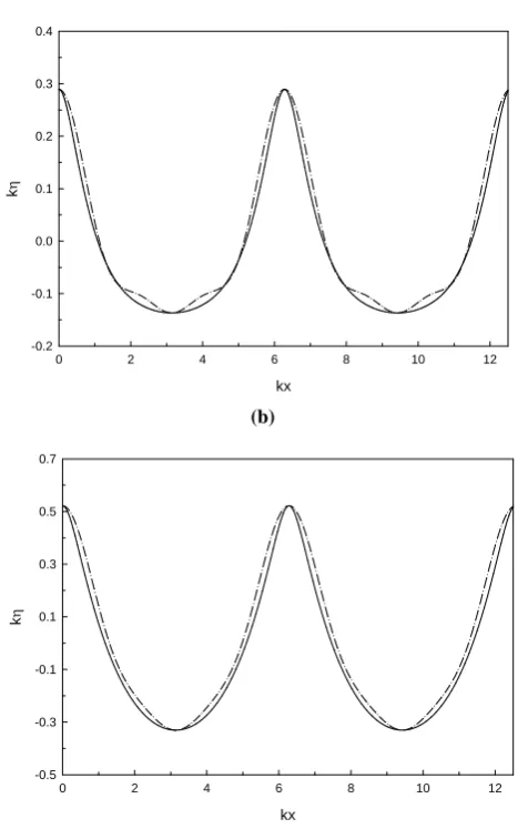
Figure 4 provides a comparison of the wave profiles be-tween Lagrangian and Eulerian solutions, both to a third-order approximation. The results reveal that the height of the wave increases against an opposing current (negative

Fr=U/c0)and decreases on a following current (positive

Fr). In Figure 4a, the Eulerian wave profiles have anomalous

bumps in the trough for the wave conditions tested, which may not be a realistic physical phenomenon for waves of con-stant form. On the other hand, the Lagrangian wave profiles have sharper crests and broader troughs, as well as exclude any artificial bumps at or near the trough. Clearly the third-order Lagrangian solution is more exact than the Eulerian solution of the same order for describing the shape of the gravity wave. In general, the surface profile is an unknown function in the Eulerian approach, and the boundary condi-tions at the free surface can only be satisfied in an approxi-mately manner. However, the free surface in the Lagrangian description is represented explicitly by a parametric function for the particles. The advantage of using Lagrangian descrip-tion is that it allows flexibility for capturing the actual shape and the wave kinematics above mean water level. Thus the-oretically, Lagrangian solution can provide better prediction for the wave profile at a large Froude number than the Stokes’ expansion to the same order. The wave profiles depicted in

(a)

kx

0 2 4 6 8 10 12

k



-0.2 -0.1 0.0 0.1 0.2 0.3 0.4

(a)

kx

0 2 4 6 8 10 12

k



-0.5 -0.3 -0.1 0.1 0.3 0.5 0.7

(b)

Figure 4. A comparison on the wave profiles for the Eulerian and Lagrangian

solutions both to a third-order under different current conditions (a) , (b)

. Wave conditions

0.3

r

F 

0.2

r

F   d L/ 0.2 and H L/ 0.1 (Solid line: third-order

Lagrangian solution; dash-dotted line: third-order Eulerian solution)

(b)

kx

0 2 4 6 8 10 12

k



-0.2 -0.1 0.0 0.1 0.2 0.3

(a)

kx

0 2 4 6 8 10 12

k



-0.5 -0.3 -0.1 0.1 0.3 0.5 0.7

(b)

Figure 4. A comparison on the wave profiles for the Eulerian and Lagrangian

solutions both to a third-order under different current conditions (a) , (b)

. Wave conditions

0.3

r

F 

0.2

r

F   d L/ 0.2 and H L/ 0.1 (Solid line: third-order

Lagrangian solution; dash-dotted line: third-order Eulerian solution)

Fig. 4. A comparison on the wave profiles for the Eulerian and Lagrangian solutions both to a third-order under different current conditions (a)Fr=0.3, (b)Fr= −0.2. Wave conditionsd/L=0.2 andH /L=0.1 (Solid line: third-order Lagrangian solution; dash-dotted line: third-order Eulerian solution).

Fig. 4 also show that they are symmetric with respect to the crest line, which were recently proven to hold true for irrota-tional waves

(a) TE=0.99sec ,H=4.62cm ,d=50cm ,b=0cm , U=2.95cm/sec (b) TE=1sec ,H=13.20cm ,d=80cm ,b=0cm , U=9.63cm/sec

(c) TE=1.39sec ,H=15.20cm ,d=80cm ,b=0cm , U=8.93cm/sec (d) TE=2.06sec ,H=5.82cm ,d=80cm ,b=0cm , U=11.72cm/sec

(e) TE=0.96sec ,H=5.23cm ,d=50cm ,b=0cm , U= -5.94cm/sec (f) TE=0.96sec ,H=6.81cm ,d=50cm ,b=0cm , U= -6.60cm/sec

The present theory Experiment

60

50 40

30 20

10 1

1 20 40 60

(cm) (cm)

30 50

10

Experiment The present theory

Experiment The present theory

1

1 20 20 40 60

40 60

(cm) (cm)

50 _{10 30}

(cm) (cm)

The present theory Experiment

50 30

10

30 10

50 10

30

50 70

80 40

60 20 1

Experiment

40 60

20

Experiment

The present theory ₁

The present theory

(g) TE=1.66sec ,H=4.20cm ,d=50cm ,b= -9.5cm , U= -7.14cm/sec (h) TE=0.93sec ,H=3.17cm ,d=50cm ,b= 0cm , U= -21.01cm/sec

Experiment The present theory Experiment

The present theory

10

30 10

(cm) (cm)

20

1

20 1

Figure 5a~5h Comparisons between the orbits of water particles obtained by the

presented theory and those from the experimental measurements of the PS motions at

different water levels b in the various experimental wave cases, where solid line is the

theoretical result and point is the experimental data which the time interval between

particle advances a distance forward, which is commonly re-ferred to as mean horizontal drift or mass transport in the direction of wave propagation. The water particle at the free surface (b=0) travels fastest, whilst that in the interior of the fluid propagates slower. To the third-order approxima-tion, the particle trajectory has non-closed orbit, irrespective of their initial mean locations. This confirms the theoreti-cal results obtained in Constantin (2006) and Constantin and Strauss (2010) for waves of large amplitude.

In the case of wave on a following current, the effect of in-creasing current speed is generally to augment the magnitude and extent of the time-averaged drift velocity, thus resulting in large horizontal distance traveled by a particle compared with the case without current. Again, the converse is true when a wave train encounters an opposing current, which retards the advancement of water particles compared to that without a current or with a following current. As the strength of an opposing current becomes comparable with the wave speed, the water particle at greater depths beneath the still water level is mainly transport by the opposing current in larger current velocity and the direction of particle movement becomes contrary to wave progression. Figure 5a–h show ex-cellent agreements between the measured trajectory and the theoretical trajectory predicted by the present third order La-grangian wave theory. This is also in agreement with the theoretical findings in Constantin and Strauss (2010).

6 Conclusions

A particle-specific description of irrotational finite-amplitude progressive gravity waves on a uniform current in water of uniform depth satisfying all the governing equations and the boundary conditions is presented. The new Lagrangian so-lution is obtained to the third order. It can be used not only to determine the wave properties available in the Eulerian solution, but also to get the trajectory, the period, the mass transport and the Lagrangian mean level of a water particle, which are not available from the Eulerian solution. In the Lagrangian solution to a second-order, the Lagrangian mean level of a particle orbit over its motion period is found to be higher than that of the Eulerian, and it also has a time-dependent term referred to as the mass transport velocity, which is applicable to the entire flow field. The frequency associated with water particle motions in Lagrangian form differs from that of the Eulerian, and the former is a function of wave steepness, uniform current speed and the Lagrangian vertical marked labelb for each individual particle that can be obtained directly based on the third-order solutions.

From the trajectories of water particles resulting from wave-current interaction, it is found that particle displace-ment near the surface decreases due to its mass transport velocity is resisted by an opposing current. Again in the case with an opposing current, the water particle further be-neath the still water level is mainly transported by the

op-posing current in the direction against the progressive wave, especially with a current in the large Froude numberFr. In

the cases with a following current, the effect of increasing current speed is generally to increase the magnitude of the time-averaged mass transport velocity since the current is in the same direction as the wave propagation, thus resulting in augmentation to the horizontal distance traveled by a particle. Finally, a set of experiments analyzing the Lagrangian prop-erties of nonlinear wave-current interaction flow is conducted in the wave tank. It shows excellent agreement between the experimental and theoretical results, including particle tra-jectories, Lagrangian wave frequency, mass transport veloc-ity and Lagrangian mean water level predicted by the present third-order Lagrangian solution.

Acknowledgements. The authors thank the anonymous referees for invaluable comments. This work was supported in part by the NSC grants 101-2911-I-110-504, 101-2622-E-006-010-CC2 and 99-2923-E-110-001-MY3 in Taiwan.

Edited by: C. Kharif

Reviewed by: H. B. Branger and another anonymous referee

References

Biesel, F.: Study of wave propagation in water of gradually varying depth, Gravity Waves, US National Bureau of Standards, Circu-lar 521, 243–253, 1952.

Brevik, I.: Flume experiment on waves and current II, Smooth bed, Coast. Eng., 4, 149–177, 1980.

Buldakov, E. V., Taylor, P. H., and Eatock Taylor, R.: New asymp-totic description of nonlinear water waves in Lagrangian coordi-nates, J. Fluid Mech., 562, 431–444, 2006.

Chen, Y. Y., Hsu, H. C., Chen, G. Y., and Hwung, H. H.: Theoret-ical analysis of surface waves shoaling and breaking on a slop-ing bottom, Part 2 Nonlinear waves, Wave Motion, 43, 356–369, 2006.

Chen, Y. Y. and Hsu, H. C.: Third-order asymptotic solution of non-linear standing water waves in Lagrangian coordinates, Chinese Physics B., 18, 861, 2009.

Chen, Y. Y., Hsu, H. C., and Chen, G. Y.: Lagrangian experi-ment and solution for irrotational finite-amplitude progressive gravity waves at uniform depth, Fluid Dyn. Res., 42, 045511, doi:10.1088/0169-5983/42/4/045511, 2010.

Clamond, D.: On the Lagrangian description of steady surface grav-ity waves, J. Fluid Mech. 589, 433–454, 2007.

Constantin, A.: Edge waves along a sloping beach, J. Phys. A, 34, 9723–9731, 2001.

Constantin, A.: On the deep water wave motion, J. Phys. A, 34, 1405–1417, 2001.

Constantin, A. and Strauss, W.: Exact steady periodic water waves with vorticity, Commun. Pure Appl. Math., 57, 481–527, 2004. Constantin, A.: The trajectories of particles in Stokes waves, Invent.

Math. 166, 523–535, 2006.

Constantin, A.: On the particle paths in solitary water waves, Q. Appl. Math., 68, 81–90,2010.

Constantin, A. and Escher, J.: Analyticity of periodic traveling free surface water waves with vorticity, Ann. Math., 173, 559–568, 2011.

Gerstner, F. J.: Theorie de wellen, Abh. d. K. bohm. Ges. Wiss., reprinted in Ann der Physik 1809, 32, 412–440, 1802.

Hsu, H. C., Chen, Y. Y., and Wang, C. F.: Perturbation analysis of short-crested waves in Lagrangian coordinates, Nonlinear Anal-ysis: Real World Application, 11, 1522–1536, 2010.

Jonsson, I. G.: Wave-current interaction, The Sea, Ocean Eng. Se-ries, 9, 1990.

Kemp, P. H. and Simons R. R.: The interactions of waves and a turbulence current: waves propagating with the current, J. Fluid Mech., 116, 227–250, 1982.

Kemp, P. H. and Simons R. R.: The interactions of waves and a tur-bulence current: waves propagating against the current, J. Fluid Mech., 130, 73–89, 1988.

Lamb, H.: Hydrodynamics, 6th ed. Cambridge University Press, 1932.

Longuet-Higgins, M. S.: Mass transport in water waves, Philos. T. R. Soc. A, 245, 533–581, 1953.

Longuet-Higgins, M. S.: The trajectories of particles in steep, sym-metric gravity waves, J. Fluid Mech., 94, 497–517, 1979. Longuet-Higgins, M. S.: Eulerian and lagrangian aspects of surface

waves, J. Fluid Mech., 173, 683–707, 1986.

Miche, A.: Mouvements ondulatoires de la mer en profondeur con-stante ou d´ecroissante, Annales des ponts et chaussees, 25–78, 131–164, 270–292, 369–406, 1944.

Naciri, M. and Mei, C. C.: Evolution of a short surface wave on a very long surface wave of finite amplitude, J. Fluid Mech., 235, 415–452, 1992.

Ng, C. O.: Mass transport in gravity waves revisited, J. Geophys., Res., 109, C04012, doi:10.1029/2003JC002121, 2004.

Peregrine, D. H.: Interaction of water waves and currents, Adv. Appl. Mech., 16, 9–117, 1976.

Pierson, W. J.: Perturbation analysis of the Navier-Stokes equations in Lagrangian form with selected linear solution, J. Geophys., Res., 67, 3151–3160, 1962.

Stuhlmeier, R.: On edge waves in stratified water along a sloping beach, J. Nonl. Math. Phys., 18, 127–137, 2011.

Rankine, W. J. M.: On the exact form of waves near the surface of deep water, Philos. T. R. Soc. A, 153, 127–138, 1863.

Sanderson, B.: A Lagrangian solution for internal waves, J. Fluid Mech., 152, 191–137, 1985.

Thomas, G. P.: Wave-current interactions: an experimental and nu-merical study, Part 1. Linear waves, J. Fluid Mech., 110, 457– 474, 1981.

Thomas, G. P.: Wave-current interactions: an experimental and nu-merical study. Part 2, Nonlinear waves, J. Fluid Mech., 216, 505– 536, 1990.

Thomas, G. P. and Klopman G.: Wave-current interactions in the near-shore region, Adv. Fluid. Mech Ser., Computational Me-chanics Publications, 66–84, 1997.

Umeyama, M.: Coupled PIV and PTV measurements of particle velocities and trajectories for surface waves following a steady current, J. Waterw. Port C-ASCE, 137, 85–94, 2010.