www.nonlin-processes-geophys.net/21/49/2014/ doi:10.5194/npg-21-49-2014
© Author(s) 2014. CC Attribution 3.0 License.
Nonlinear Processes
in Geophysics
The Rossby wave extra invariant in the dynamics of 3-D fluid layers
and the generation of zonal jets
A. M. Balk
Department of Mathematics, University of Utah, Salt Lake City, UT 84112, USA Correspondence to: A. M. Balk ([email protected])
Received: 28 February 2013 – Revised: 22 September 2013 – Accepted: 9 November 2013 – Published: 10 January 2014
Abstract. We consider an adiabatic-type (approximate)
in-variant that was earlier obtained for the quasi-geostrophic equation and the shallow water system; it is an extra invari-ant, in addition to the standard ones (energy, enstrophy, mo-mentum), and it is based on the Rossby waves. The presence of this invariant implies the energy transfer from small-scale eddies to large-scale zonal jets.
We show that this extra invariant can be extended to the dynamics of a three-dimensional (3-D) fluid layer on the beta plane. Combined with the investigation of other researchers, this 3-D extension implies enhanced generation of zonal jets. For a general physical system, the presence of an extra invariant (in addition to the energy–momentum and wave ac-tion) is extremely rare. We summarize the unique conserva-tion properties of geophysical fluid dynamics (with the beta effect) that allow for the existence of the extra invariant, and argue that its presence in various geophysical systems is a strong indication that the formation of zonal jets is indeed related to the extra invariant.
Also, we develop a new, more direct, way to establish ex-tra invariants (without using cubic corrections). For this, we introduce the small denominator lemma.
1 Introduction
Alternating zonal jets are found in the large-scale dynamics of oceans and atmospheres under broad conditions. Clearly seen on Jupiter, zonal jets are also unambiguously observed in Earth’s oceans (Maximenko et al., 2005). The significance of zonal jets also stems from the well-known mathematical analogy between rotation and magnetic field. Similar equa-tions and similar jets also appear in the dynamics of magne-tized plasmas; these jets serve as transport barriers in toka-maks, improving conditions for the controlled nuclear fusion with magnetic confinement (e.g., Manz et al., 2012).
The emergence of zonal jets has been and continues to be intensively studied in both geophysical and plasma contexts. The main purpose of the present paper is to draw attention to the fact that the equations used to describe zonal jets have an unusual adiabatic-like (approximate) invariant (in addi-tion to the usual energy–momentum); this makes the inverse cascade anisotropic and leads to the energy transfer towards zonal jets (see Sect. 4.2). As will be clear below (Sect. 2), this extra invariant is very rare: almost all other physical systems do not have anything analogous to such an invariant. The presence of this conservation in various geophysical systems (within the beta-plane approximation) is a strong indication that the extra invariant indeed plays a role in the emergence of zonal jets.
At this point, it is beneficial to recall two seemingly unre-lated problems (Sects. 1.1 and 1.2). Then in Sect. 2, we de-scribe the extra invariant and summarize the corresponding unique conservation properties of geophysical systems that allow for its existence. This summary includes the extension of the extra invariant to 3-D fluid layers, which is derived in the present paper (Sect. 3). We see how this invariant implies the energy cascade towards zonal jets in Sect. 4.
1.1 Boltzmann’s collision invariants
Introducing his kinetic equation, L. Boltzmann (1875) in-vestigated the general form of the thermodynamic equilib-rium (Maxwell distribution). Boltzmann studied rarefied gas when the main interaction between the molecules are bi-nary collisions. In each collision, momenta of two molecules before (p1,p2) and after (p3,p4) the collision satisfy the
momentum–energy conservation:
p1+p2=p3+p4, p12+p22=p23+p24. (1)
These relations imply the conservation of the total momen-tum and energy
P=
Z
pNpdp, E=
Z
p2Npdp, (2)
where Np is the particle distribution function (the
num-ber of molecules with momentump). The total number of molecules
N=
Z
Npdp (3)
is also conserved, which corresponds to the obvious relation 1+1=1+1 for each binary collision.
Boltzmann posed the following question: does there exist another functionϕ(p)that is also conserved in binary colli-sions, so that the relations in Eq. (1) imply the relation ϕ (p1)+ϕ (p2)=ϕ (p3)+ϕ (p4) ? (4)
In other words, does there existϕ(p), such that Eq. (4) holds for any four vectorsp1,p2,p3,p4, bound by Eq. (1)? Then
Boltzmann’s kinetic equation would additionally conserve the integral
I=
Z
ϕ (p) Npdp. (5)
It is supposed that the functionϕ(p)is linearly independent of the five functions: 1, three components ofp, andp2, so that the quantity (5) is independent of quantities (2) and (3).
If there were such a function ϕ(p), then the thermody-namic equilibrium would be different. However, Boltzmann (1875) found that there is no such a functionϕ(p)(provided it is smooth enough; see also Sercignani, 1990).
1.2 Zakharov–Schulman test of integrability: degenerative dispersion laws
In a different development, Zakharov and Schulman (1980, 1988) posed the question “When a given nonlinear wave sys-tem is integrable?” They argued that, to be integrable, the system should possess an additional conservation law, be-sides the energy and the momentum (and, sometimes, the wave action).
Suppose our nonlinear wave system is given in the Fourier representation as dynamics of wave amplitudesak(t )
i ∂
∂tak1=ω (k1) ak1+
1 2
Z
V (k1,k2,k3)
ak2ak3δ (k1−k2−k3)dk2dk3+. . . , (6)
so that the time derivative of a wave amplitude (with some wave vector k1) is determined by the contributions of all
other waves. The dispersion lawω(k)determines the linear part of Eq. (6), and the coupling coefficient V (k1,k2,k3)
determines quadratic nonlinearity. The dots stand for other nonlinear terms; these are other quadratic terms (namely, the ones containingaa∗anda∗a∗;∗denotes complex conjuga-tion), as well as higher order nonlinearity terms. The sys-tem is obviously translationally symmetric with respect to shifts in time (since all coefficients are time-independent), so it conserves the energy. The system is also translationally symmetric with respect to shifts in space, due to the presence of the delta function of the wave vectors (it just provides a way to write the convolution), so the system conserves mo-mentum.
Zakharov and Schulman assumed that the wave ampli-tudes are chosen to be canonical Hamiltonian variables, so that the dynamical Eq. (6) has the form
i∂ ∂tak=
δH
δa∗k (7)
with some HamiltonianHexpanded in a series over powers of wave amplitudes
H=
Z
ω (k) akak∗dk
+1 2
Z
V (k1,k2,k3) a∗k1ak2ak3δ (k1−k2−k3)dk2dk3
+ {c.c.} + {. . .other nonlinear terms. . .} (8) ({c.c.}means the complex conjugated term). Then the mo-mentum is
P=
Z
kakak∗dk, (9)
law: I=
Z
ϕ (k) aka∗kdk
+1 2
Z
F (k1,k2,k3) ak1∗ ak2ak3δ(k1−k2+k3)dk2dk3
+ {c.c.} + {. . .other nonlinear terms. . .} (10) (with undeterminedϕ,F, and so on); ϕ is supposed to be linearly independent of k and ω, so that I is independent of the momentum and energy. They found that in order for Eq. (10) to be conserved by the dynamics in Eq. (7)–(8), the following alternative should hold. At least one of the two conditions are to be satisfied:
1. The function ϕ (k)is conserved in the resonant triad interactions: the equation
ϕ (k1)=ϕ (k2)+ϕ (k3) (11)
holds for all vectorsk1,k2, andk3bound by the
reso-nance relations
k1=k2+k3, ω (k1)=ω (k2)+ω (k3) . (12)
2. Or the resonant triad interaction is impossible. This can happen in two ways: Eq. (12) can have no solutions (like it happens for the gravity waves); or the nonlinear coupling coefficientV (k1,k2,k3)can identically
van-ish on the resonance manifold defined by Eqs. (12). Introducing the classical scattering matrix, Zakharov and Schulman (1988) obtained other necessary conditions for the conservation of Eq. (10). These are equations on F (k1,k2,k3) and other kernels of higher order nonlinear
terms in Eq. (10). They demonstrated (1980; 1988) their arguments on several integrable systems, in particular, the Kadomtsev–Petviashvili equation.
They also called the dispersion lawω(k)– which admits the additional conservation in Eq. (11) – degenerative.
The Zakharov–Schulman Eq. (11) and (12) for nonlinear waves are similar to Boltzmann’s Eqs. (4) and (1) for rarefied gas, but waves provide a bigger variety:
a. The main interactions can involve any number of waves, in particular, only three waves (like in Eqs. 11– 12).
b. There are many forms of the dispersion law, not just the quadratic functionω(k)=k2(like in Boltzmann’s case).
c. The physically interesting media (in which the waves propagate) can have different dimensions of d= 1,2,3.
2 Unique conservation properties of large-scale geophysical fluid dynamics
2.1 Quasi-geostrophic equation
The Rossby wave dispersion law turned out to be degenera-tive (Balk et al., 1991; Balk, 1991).
When dispersion law has the form ω(k)= − β p
α2+k2
h
k=(p, q), k2=p2+q2i (13) (αandβare parameters), the resonance relations in Eq. (12) imply Eq. (11) withϕ(k)equal to the function
η (k)≡arctan
αq+p √
3
k2 −arctan
αq−p √
3
k2 (14)
(Balk, 1991). The conservation of the function in Eq. (14) in triad resonances implies that the quasi-geostrophic equation
1ψ−α2ψ
t
+βψx+ψy1ψx−ψx1ψy=0 (15)
possesses an approximate invariant I=1
2
Z 1
pη(k)|Qk(t )|
2dpdq, (16)
withQk(t )being the Fourier transform of
Q(x, y, t )=1ψ−α2ψ. (17) The function in Eq. (14) is conserved exactly in resonant triad interactions, but the integral in Eq. (16) is conserved approximately in all interactions (including triads that are far from being resonant). (If typical length scaleL and pa-rameterβare normalized to 1, andεis a characteristic non-dimensional wave amplitude, then the invariant in Eq. (16) has a magnitude ofO(ε2), while its variation1I≡I (t )− I (0)has a smaller magnitude of1I=O(ε3)on long time intervalsO(1/ε); see Balk and van Heerden, 2006, for de-tails.)
Ferapontov (1992) realized that the problem of collision invariants (for rarefied gas, Sect. 1.1) and the problem of de-generative dispersion laws (for nonlinear waves, Sect. 1.2) can be posed as a problem of web geometry, which has been developing since the 1920s (Blaschke, 1932).
In particular, using the web geometry results, it is possi-ble to show (Balk and Ferapontov, 1998) that the function in Eq. (14) is unique: any functionϕ(k), conserved in triad res-onances in Eq. (12) – with the Rossby dispersion lawω(k)– is a linear combination ofk,ω (k), andη(k).
The connection to the web geometry also shows how ex-ceptional the systems with extra invariants are. As one can guess, it is rare that four Eqs. (11) and (12) (the first equa-tion in (12) consists of two scalar equaequa-tions) in the six-dimensional space of wave vectorsk1, k2,k3 determine a
Even though Eq. (11) follows from the resonance relations in Eq. (12) (Eq. 11 is only linearly independent of Eq. 12), the integral (Eq. 16) is completely independent of the stan-dard invariants (energy–momentum), because the integrand containsQk(t ).
The presence of the extra invariant in Eq. (16) implies the energy transfer from small-scale eddies to large-scale zonal jets (Balk, 2005).
This is often but not always the case: the extra invariant does not lead to zonal jets, when the energy source is on large scales (i.e., the forcing scalekfis long-wave,kfα). In the
latter situation, the energy accumulates in the sectors of polar anglesθ=arctan(q/p)such that 60◦<|θ|<90◦. However, in the present paper we do not need to deal with this, since we are concerned with the opposite situationkαfor allk. Ask→ ∞, the extra invariant function in Eq. (14) and the dispersion law in Eq. (13) turn out to be asymptotically pro-portional (the same propro-portionality in all directionsk/ k!); a certain linear combination of Eqs. (14) and (13), which can-cels the common asymptotics, gives an extra invariant
5 4α4
η (k)
2 √
3α
+ω (k) β
∼p
3 p2+5q2
k10 , (kα) . (18)
This linear combination decreases much faster with|k|than both functions in Eq. (14) and (13); the energy transfer to-wards zonal jets turns out to be more pronounced in the short-wave case (see Balk, 2005, for details of long- and shortshort-wave limits).
Nazarenko and Quinn (2009) demonstrated the conserva-tion of the extra invariant in Eq. (18) in the numerical simu-lations of the quasi-geostrophic equation.
2.2 Shallow water system
The extra invariant in Eq. (16) was extended (Balk et al., 2011) to the shallow water system on the beta plane
ut+u ux+v uy−f (y) v = −g Hx,
vt+u vx+v vy+f (y) u= −g Hy, (19)
Ht+(H u)x+(H v)y =0,
where (u, v) is the horizontal fluid velocity, H the fluid height (flat bottom is assumed),g the gravity acceleration, andf (y)the Coriolis parameter. The shallow water system in Eq. (19) adiabatically conserves the integral in Eq. (16), withQk(t )being the Fourier transform of the perturbational
potential vorticity (e.g., Gill, 1982)
Q(x, y, t )=vx−uy−f (y)h, (20)
where h=(H−H0)/H0 is the fractional relative height,
which measures the deviation of the fluid surface height H (x, y, t )from its unperturbed valueH0.
The extension was possible due to the following two unique conservation properties of Eq. (19).
First, the shallow water dynamics in Eq. (19) – besides Rossby waves – contains the inertia–gravity (IG) waves. The former could (in general) leak energy to the latter, thereby de-stroying the conservation of the extra invariant in Eq. (16) – which is based only on Rossby waves. However, the coupling coefficient of triad interaction between the IG and the Rossby waves vanishes, provided the Coriolis parameter is constant. Iff (y)varies sufficiently slowly (i.e.,β(y)≡f0(y)is suf-ficiently small), then the extra invariant slowly changes due toβ6=0, but within its non-conservation due to the quar-tet interactions (recall that the invariant is only adiabatically conserved and can slowly change).
Second, the beta plane in Eq. (19) can be not only mid-latitudinal but also close to the Equator. As we approach the Equator, the Coriolis parameter decreases, and the quasi-geostrophic approximation becomes invalid. Correspond-ingly, in the perturbation expansions, the Coriolis parame-terf enters the denominators. However, the specific form of Eq. (19) makes it possible to refine (Balk et al., 2011) the Rossby mode, so that the numerators (in the perturbation ex-pansion) are equally small in the limitf →0.
2.3 3-D fluid layers
2.3.1 Motivation
The application of the extra invariant in Eq. (16) to the real oceans and atmospheres of rotating planets encounters the following natural question. In a fluid layer of finite depthH, the shallow water motions (which are two-dimensional, 2-D) can generate – due to nonlinearity – the 3-D inertia waves. One can argue that the length of a typical Rossby wave sig-nificantly exceeds the depthH, so the energy exchange be-tween Rossby waves and inertia waves can be disregarded due to the disparity of scales. But the question remains for short Rossby waves, whose wavelength can be comparable to the depthH; they could effectively interact with 3-D modes. Even if the energy of short Rossby waves were small, they could gradually leak significant amount of energy during long time evolution.
At the same time, the extra conservation seems to be es-sentially tied to the two-dimensionality or, more generally, to low dimension. So far, extra invariants have been found in two situations: (1) triads in 2-D media (see Eq. 12) and (2) quartets in 1-D media (Balk and Ferapontov, 1993), e.g., p1+p2=p3+p4, ω(p1)+ω(p2)=ω(p3)+ω(p4) (21)
(pis the wave number in the 1-D media). In both situations, a wave with some fixed wave vector (say,k1orp1) participates
in only one-dimensional family of resonant interactions. Let us elaborate. The triad resonance relations in Eq. (12) for 2-D wave vectors define manifold of dimension 3. A wave with a fixed wave vector (say,k1) can be involved with only
vector (sayp1) participates again in one-dimensional family
of resonant interactions.
For 3-D media, the triad resonance relations in Eq. (12) define manifold of dimension 5; a fixed wave vector (say,k1)
is involved in two-dimensional family of resonance triads. There is an example of extra invariants for triad interaction in 3-D media (Balk, 1997), but it seems somewhat artificial.
Nevertheless, the extra invariant in Eq. (16) can be ex-tended to the 3-D dynamics. This is due to the special prop-erty of the fluid equations, which was found a long time ago (Greenspan, 1969).
2.3.2 Problem
Since the short Rossby waves are the prime candidates for the energy exchange with 3-D modes, we consider the 3-D dynamics in the well-known classical situation (e.g., Landau and Lifshitz, 1987) of ideal incompressible (with constant densityρ0) rotating fluid
vt+(v· ∇)v+f×v= −∇5,
∇ ·v=0, (22)
wherev=(u, v, w)is the fluid velocity;5is the fluid pres-sure (centrifugal force included) divided byρ0. Euler’s
equa-tion (Eq. 22) involves Coriolis force, withfbeing the double angular velocity. The fluid is assumed to occupy a layer be-tween two parallel horizontal planes, rotating about vertical axisz. The boundary condition is vanishing of the vertical fluid velocity at the solid plane boundaries
w(x, y,0, t )=w(x, y, H0, t )=0. (23)
The Coriolis parameter slowly changes with the meridional coordinatey:
f=(0,0, f ), f =f0+βy. (24)
The system in Eq. (22) describes the dynamics of inertia waves and vortical mode (e.g., Landau and Lifshitz, 1987, §14); the latter – due to the dependence off ony – repre-sents short Rossby waves with dispersion law
(k)= −βp k2
k=(p, q)
.
Greenspan (1969) discovered that on thef plane (when β=0), the inertia modes do not produce triad-resonant re-sponse on the geostrophic mode. In other words, in the equa-tion for the geostrophic mode (which has zero frequency), the coupling coefficient between this mode and two iner-tia modes (with frequencies ωm and ωn) vanishes
when-everωm+ωn=0. It is reasonable to think that for nonzero
– but sufficiently small – β, the triad resonant response is sufficiently small, so the second condition of Zakharov– Schulman’s alternative (Sect. 1.2) is realized approximately: V (k1,k2,k3)on the triad resonance manifold is not zero but
“small”. Then, the rapidly rotating 3-D fluid dynamics ap-pears to have the invariants of the 2-D shallow water dynam-ics. In Sect. 3 this is derived explicitly.
2.3.3 Result
LetL be the length scale,U0 the velocity scale, andf0=
f (0)the reference value of the Coriolis parameter. We use two small parameters:
– First, the Coriolis parameterf (y)is a slow function: the variation1f≡f−f0∼βLis small compared to
f0
βL f0
1.
This condition means that L is much less than the Earth radiusR0, since at midlatitudes,β∼f0/R0. – Second, we consider weakly nonlinear dynamics,
when the nonlinear terms are small compared to the linear terms. This means nonlinearity being small compared to the beta effect, namely,
= U0 βL21.
We need this, even though the Euler equation (Eq. 22) contains a linear term withf. Indeed, later (Sect. 3.2), we consider Eq. (33) for the vertical component of vor-ticity. We integrate Eq. (33) over the fluid depth, and the f term disappears (due to the incompressibility ux+vy+wz=0 and boundary condition in Eq. (23)).
Then the only remaining linear term containsβ, and the typical ratio of nonlinear terms to linear term is. Let us estimate for large-scale dynamics in Earth’s oceans: flow at latitude≈30◦withU
0≈5 cm s−1and
L≈100 km has≈1/4. Is this sufficiently small to have the extra invariant? Perhaps, the weakly nonlin-ear dynamics is just a useful model that cannot be fully justified but nevertheless leads to plausible results (see also discussion of weak nonlinearity in the Introduc-tion).
At this point, we assume that the fluid equations are written in dimensionless form with timescale 1/f0and length scaleL
(in other words, the units are chosen such thatf0=L=1).
Then the dimensionless Coriolis parameter is f =1+βy with dimensionless β1; the dimensionless typical fluid velocity isU0=β.
We will derive in Sect. 3 that the dynamics in Eq. (22)– (24) possesses an invariant
I=1 2
Z p2 p2+5q2
p2+q25
|ζk(t )|2dk, (25)
wherek=(p, q)is the horizontal wave vector, andζk(t )is
the Fourier transform ofz-averaged vertical vorticity
ζ (x, y, t )= 1 H0
H0
Z
0
We will derive the following estimate for the variation of the integral in Eq. (25):
1I≡I (t )−I (0)=O2.5β2+O2β2.5, (27) and over timet=O(−1β−1). At the same time, the invari-antI has the order2β2, so1II. The period of Rossby waves isO(β−1), soI is conserved during time intervals of many – namelyO(−1)– Rossby wave periods. (An estimate stronger than Eq. (27) can be obtained with further assump-tions.)
3 Derivation
3.1 Normal mode expansion
To obtain the extra invariant in Eq. (25), let us expand the solution of Eq. (22) in normal modes of linearized system withβ=0:
ut−f0v= −5x,
vt+f0u= −5y,
wt= −5z, (28)
ux+vy+wz=0,
w(x, y,0, t )=w(x, y, H0, t )=0.
(In our dimensionless units f0=1, but we keep f0just to
see physical meaning.) There are normal modes of two types: (1) the vortical mode, representing the Taylor–Proudman col-umn
u= −1 f0
5y, v=
1 f0
5y, w=0, 5z=0, (29)
(which is t andz independent), and (2) the inertial waves (standing in thezdirection)
u v w 5 = ˆ u cosmz ˆ v cosmz
ˆ wsinmz
ˆ 5 cosmz
ei(px+qy−ωt ), (30)
wherem=nπ/H0with non-zero integer n. Substitution of
Eq. (30) into Eq. (28) gives the dispersion relation
ω2K2=f02m2 K2=p2+q2+m2, (31) and the polarization vector
ˆ u ˆ v ˆ w ˆ 5 =
−iqf0−ωp
ipf0−ωq
iω k2/m f02−ω2
.
The capitalKdenotes the full three-dimensional wave vec-tor, K=(p, q, m), while the small case k stands for the
horizontal 2-D vector, k=(p, q). The general solution of Eq. (28) is a linear combination of all normal modes with some coefficients9kandAK:
u(x, y, z, t ) v(x, y, z, t ) w(x, y, z, t ) 5(x, y, z, t )
= Z
dpdq ei(px+qy) (32)
9k −iq ip 0 f0 +X m AK
(−iqf0−ωp)cosmz
(ipf0−ωq)cosmz
(iω k2/m)sinmz (f02−ω2)cosmz
e−iωt
.
Hereω≡f0m/K; the summation in Eq. (32) is over m=
π
H0n, n= ±1,±2, . . .;9−k=9 ∗
k,A−K=A ∗ K.
The solution of the full (nonlinear and with non-zeroβ) system in Eq. (22) can also be expanded in the form (32), but the coefficients9kandAKwould depend on timet. 3.2 Equation for the vertical vorticity in terms of
normal modes
From Eq. (22) we have
vx−uyt+ uvx+vvy+wvzx − uux+vuy+wuz
y+f ux+vy
+βv=0. (33) Now we substitute Eq. (32) into Eq. (33) and integrate over z(from 0 toH0), taking into account that cosines cosmz
in-tegrate to zero. To shorten writing, any subscript wave vec-torkj orKj will be replaced by its label subindexj (e.g.,
9j ≡9kj,Aj≡AKj). This is unambiguous: indexj stands for Kj if the corresponding quantity – like A – depends
on the three-dimensional wave vectorK;j stands forkj if
the corresponding quantity – like9 – depends on the two-dimensional wave vectork. In addition,−j stands for−Kj
or−kj; d23≡dk2dk3≡dp2dq2dp3dq3.
Thus, Eq. (33) becomes k219˙1=βip191+
1 2
Z
W−1,2,39293d23
+1 2
Z X
m2,m3
V−1,2,3e−i(ω2+ω3)t A2A3d23. (34)
The integrals in Eq. (34) have been symmetrized with respect to transposition of indexes 2 and 3: this gives the factor 1/2 in front of the integrals and the symmetric coupling coefficients (W−1,2,3=W−1,3,2andV−1,2,3=V−1,3,2)
W1,2,3≡Wk1,k2,k3
=11,2,3
k23−k22δ (k1+k2+k3) , (35)
V1,2,3≡Vk1,K2,K3
= f011,2,3−iω3k1·k3(f0k1·k2−iω21123)
− f011,2,3+iω2k1·k2(f0k1·k3+iω31123)
δm2−m3+δm2+m3
Hereδ(·)is the Dirac delta function, andδmis the Kronecker
symbol (which is 1 ifm=0 and 0 ifm6=0): 11,2,3=p2q3−p3q2,
which – because of the delta function – has the following obvious symmetries:
11,2,3=12,3,1=13,1,2= −11,3,2= −13,2,1= −12,1,3.
That is,11,2,3is symmetric with respect to the three cyclic
permutations of its indexes and anti-symmetric with respect to the other three permutations. Software MATHEMATICA
has been used to obtainV in the form of Eq. (36).
3.3 Adiabatic conservation
We intend to find invariant I=1
2
Z
X(k) 9k9−kdk, [X(k)=X(−k)] (37)
(with undetermined kernelX), which are approximately con-served over a long timeO(−1β−1). This is the nonlinear time of wave interactions (since the wave amplitudes are of the order of fluid velocity, which isO( β)). To show that I (t )stays almost constant, it would be enough to show that its time derivativeI˙is sufficiently small. However, the latter is not the case:I (t ) oscillates in time (similar to adiabatic invariants in the theory of dynamical systems). The change 1I≡I (t )−I (0)is “small”, butI˙is “big”. The usual way to deal with such a situation has been the following. The quadratic integral in Eq. (37) is supplemented by cubic cor-rections, e.g., for the dynamics in Eq. (34):
Isuppl.=1 2
Z
X(k) 9k9−kdk
+
Z
Y123919293d123+
Z
Z12391A2A3d123 (38)
(X,Y, Z are undetermined kernels); I˙suppl. is required to be sufficiently small. At the end, the cubic corrections can be dropped, since they turn out to be within the variation of 1Isuppl.≡Isuppl.(t )−Isuppl.(0).
Here we develop a new, more direct, approach (without cubic corrections).
Let us, first, apply the transformation
9k=ψke−i(k)t; (39)
it removes the linear term in Eq. (34), ˙
ψ1=
1 2k12
Z
W−1,2,3ei(1−2−3)tψ2ψ3d23
+ 1 2k12
Z X
m2,m3
V−1,2,3ei(1−ω2−ω3)tA2A3d23, (40)
and leaves the invariant (37) in the old form I=1
2
Z
X(k) ψkψ−kdk.
Its time derivative is ˙
I= ˙IR + ˙Ii, (41) where
˙ IR=1
2
Z
d123
1 k12W123e
−i(1+2+3)t ψ 1ψ2ψ3,
˙ Ii=1
2
Z
d123
X
m2,m3
X1 1
k21V123ψ1e
−i(1+ω2+ω3)tA 2A3;
˙
IRandI˙i are respectively contributions toI˙resulting from the interaction between three Rossby waves and from the in-teraction between two inertia waves and one Rossby wave. In both integrals in Eq. (41), we have replacedk1by−k1and
used that the dispersion law is an odd function (−1=
−1). Our goal is to estimate the contributions to1I
result-ing fromI˙RandI˙i, and thereby show that1I I.
3.4 Small denominator lemma
The essence of the extra invariant conservation can be ex-pressed by the lemma below. Basically, we have
dI dτ =
∞
Z
−∞
F (χ , ετ ) eiχ τdχ , (42)
and need to estimate the total variation 1I≡I (τ )−I (0) over a long time interval 0≤τ ≤ε−1.
For instance, in the case of Eq. (41), the variable χ re-sults from the exponent, and the functionF is the result of all integrations whileχ is held fixed (later, when applying the lemma, we will define χ andF exactly). The function F slowly depends on timeτ, which is signified by a small parameterε(this corresponds to the slow variation of wave amplitudes). The integral in Eq. (42) is well convergent at χ→ ±∞(corresponding to the vanishing of wave ampli-tudes ask1,k2, andk3approach infinity). It is important that
the integration interval in Eq. (42) includes pointχ=0, so that the resonance (atχ→0) is present.
In general,I exhibits secular growth associated with the resonanceχ→0, and the adiabatic conservation ofI is out of the question. Indeed, assume for simplicity thatF is time independent (ε=0); then
1I=
Z
F (χ )e
iχ τ−1
iχ dχ; (43)
For LEMMA,
Suppose, there are constantsMandLsuch that ∞
Z
−∞
F (χ ,T) χ
dχ≤M, (44)
∞
Z
−∞
F χ ,T00
−F χ ,T0
dχ≤L|T00−T0| (45)
for all positiveT,T0,T00. Then
|1I| ≤(2M+L)ε−1/2 for 0≤τ≤ε−1. (46) Comment 1. The convergence of integral in Eq. (44) implies cancellation (at least partial) of the small denominatorχ. Comment 2. The constantsMandLareT-independent, but can depend onε, which will be used in the lemma applica-tions below.
Proof. We split the time interval 0≤τ≤ε−1 into many subintervals
τj−1, τj, j=1,2, . . . J
τ0=0, τJ=ε−1
,
of lengthε−1/2; there areJ=ε−1/2of them. (To make this number integer, we can consider an appropriate subsequence of ε, or we can use the integer part J= [ε−1/2] +1 with slightly shorter subintervals.) On each subinterval
dI dτ =
Z
{F χ , ετj
+F (χ , ετ )−F χ , ετj
}eiχ τdχ; Integrating this fromτj−1toτj, we have
1Ij≡I (τj)−I (τj−1)=
Z
dχF χ , ετj
iχ
eiχ τj−eiχ τj−1
+
τj
Z
τj−1
dτ
Z
dχF (χ , ετ )−F χ , ετj
eiχ τ.
In the latter integral, |ετ−ετj| ≤ε1/2. According to
esti-mates in Eq. (44)–(45),
|1Ij| ≤2M+ τj
Z
τj−1
Lε1/2dτ=2M+L.
Now, |1I| ≤PJ
j=1|1Ij| ≤(2M+L)J, and we find
Eq. (46).
3.5 Interaction between three Rossby waves
Now we estimate1I resulting fromI˙Rin Eq. (41).
The periods of Rossby waves areO(β−1), and we intro-duce function
σ (k)= −p
k2, so that (k)=βσ (k) . (47)
Rossby wave amplitude ψk evolves on the nonlinear
timescaleO(−1β−1)(recall the transformation in Eq. (39)). Therefore, to apply the lemma of Sect. 3.4, we assume χ= −(σ1+σ2+σ3) , τ=βt, ε=.
Now, dIR
dτ = 1 β ˙ IR=
Z
F (χ , τ ) eiχ τdχ , with (48) F = 1
2β
Z
d123δ (σ1+σ2+σ3+χ )
X1
k12W123ψ1ψ2ψ3.
We symmetrize the integral forF with respect to permuta-tions of indexes 1, 2, and 3 (this, in particular, gives an addi-tional factor 1/3 in front of the integral) and use Eq. (35) for the kernelW, taking into account that11,2,3 is symmetric
with respect to the cyclic permutations of its indexes F = 1
6β
Z
d123δ (k1+k2+k3) 11,2,3ψ1ψ2ψ3
δ (σ1+σ2+σ3+χ )
"
X1
k12
k32−k22
+X2
k22
k12−k32
+X3
k23(k
2 2−k12)
#
. (49)
Now we will determine special functionsX(k)so that the integral (44) converges asχ→0. Due to the dispersion re-lation, k2j= −pj/σj(j=1,2,3), so the square bracket in
Eq. (49) equals
[. . .] = 1 σ1σ2σ3
"
p1X1
k14 (p3σ2−p2σ3)
+ p2X2 k24 (p1σ3
−p3σ1)+
p3X3
k43 (p2σ1
−p1σ2)
#
. (50)
We have p1+p2+p3=0 due to the delta function in
Eq. (49); whenχ=0, thenσ1+σ2+σ3=0, and the three
pairs of parentheses in Eq. (50) turn out equal. Now the square bracket in Eq. (49) is
[. . .] =p2σ1−p1σ2 σ1σ2σ3
"
p1X1
k41 + p2X2
k24 + p3X3
k43
#
; (51)
it vanishes if the function ϕ(k)=p X(k)
k4
is conserved in resonant triad interactions k1+k2+k3=0
1+2+3=0
⇒ ϕ1+ϕ2+ϕ3=0. (52)
Then the integral in Eq. (44) is convergent. Since ψk=
Remark.(k)andϕ(k)are odd functions of the wave vec-tork, so (implication (52)) is equivalent to the implication of Eqs. (12)⇒(11).
There are five possible functionsϕ(k)that satisfy Eq. (52). Three of them are obvious and common:
ϕ(k)=(k), ϕ(k)=p, ϕ(k)=q. (53) The other two (Balk, 1991) are specific for short Rossby waves:
ϕ(k)=ξshort(k)≡pq
k4; (54)
ϕ(k)=ηshort(k)≡p
3(p2+5q2)
k10 . (55)
Similar to Balk et al. (2011), we discard the third and the fourth of them as unphysical: the third gives singularX(k)= qk4/p (on the line p=0), and the fourth is even, giving odd X(k), which contradicts to the bracketed condition in Eq. (37). The first function in Eq. (53) corresponds to the en-ergy of the quasi-geostrophic mode; the second corresponds to the zonal momentum (which is the enstrophy).
The fifth function (Eq. 55) gives the extra invariant (cf. Eq. 18).
3.6 Interaction between one Rossby wave and two inertia waves
Now, we estimate the variation 1I resulting from I˙i in Eq. (41).
The inertia wave amplitudeAk(t )evolves faster than the
Rossby wave amplitude ψk(t ). The latter evolves on the
nonlinear timescaleO(−1β−1). The former have linear re-sponse to the Rossby waves. Recall that we used normal modes for β=0, so Ak and ψk are independent in
lin-earized dynamics if β=0 only. If β6=0, the amplitude Ak(t )evolves on timescaleO(β−1). Therefore, we use the
lemma of Sect. 3.4 with
χ= −(ω2+ω3) , τ =t, ε=β.
Now, dIi
dt =
Z
F (χ , βt ) eiχ tdχ , (56) where
F =1 2
Z
d123
X
m2,m3
δ (ω2+ω3+χ )
X1
k12V12391A2A3.
To apply the lemma, we show that the integral in Eq. (44) converges asχ→0. Indeed, whenχ=0, thenω2+ω3=0,
which implies|ω2| = |ω3|. Because of Kronecker deltas in
Eq. (36), we have|m2| = |m3|. Therefore, – by the dispersion
relation in Eq. (31) –K2=K3, andk2=k3. Now,
k2= −k1−k3 ⇒ k22=k21+k32+2k1·k3,
k3= −k1−k2 ⇒ k32=k21+k22+2k1·k2.
Thusk1·k3=k1·k2, and in the square bracket of Eq. (36),
the four pairs of parentheses are pairwise identical. There-fore,V1,2,3=0.
The wave amplitudes9 andAareO(β), and, therefore, the constantsMandLareO(3β3). Now, according to the lemma,1I=O(3β2.5)on any time interval of lengthβ−1. We can split the time interval 0≤t≤−1β−1 into subin-tervals of lengthO(β−1); there areO(−1)of them. Thus, 1I=1
O(
3β2.5)on time interval 0≤t≤−1β−1.
Combining this estimate and the estimate found in the pre-vious Sect. 3.5, we find Eq. (27).
Remark. The estimate in Eq. (27) holds for any solution of the 3-D layer dynamics in Eq. (22)–(24). If the wave turbu-lence were considered, the estimate would hold for any real-ization, even the least probable; on average (or for a typical realization) the estimate is stronger.
4 Emergence of zonal jets
4.1 Invariants
According to the expansion in Eq. (32), the vertical vorticity in Eq. (26) is
ζ (x, y, t )= −
Z
k29k(t ) ei(px+qy)dk (57)
(since the cosines integrate to zero); in the Fourier represen-tation, Eq. (57) meansζk= −k29k. So, we can express
inte-gral in Eq. (37) in terms ofζk:
I=1 2
Z 1
pϕ(k)|ζk|
2dk. (58)
Thus, we have three invariants:
1. The energy of the quasi-geostrophic mode (the energy of inertia waves is separate)
E=1 2
Z 1
k2|ζk|
2dk. (59)
2. The enstrophy Enstrophy=1 2
Z
|ζk|2dk. (60)
3. The extra invariant I =1
2
Z 1
pη
short(k)|ζ
k|2dk (61)
4.2 Anisotropic inverse cascade
In rapidly rotating 3-D fluids, the energy from inertia waves is transferred towards the quasi-geostrophic mode (Smith and Waleffe, 1999; Cambon et al., 2004; Staplehurst et al., 2008; Duran-Matute et al., 2013).
The conservation of the energy in Eq. (59) and the en-strophy in Eq. (60) implies the inverse cascade of the two-dimensional quasi-geostrophic energy (Rhines, 1975; Ped-losky, 1987; Vallis, 2006). This is because the energy spec-trum spreads in the Fourier space (unless the initial condi-tions are very specially arranged); the spreading happens due to (Rhines, 1975) the decay instability (when a wave decays into the other two waves of a resonant triad), as well as due to the resonant generation of higher harmonics.
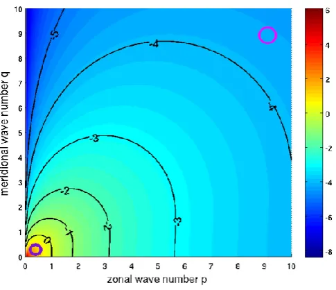
We assume that the inverse energy cascade takes place. Then the presence of the third, extra, invariant in Eq. (61) implies the energy transfer towards large-scale zonal flow, not just to large scales in general, but specifically into the region of thekplane around theqaxis. This is the only way to keep the extra invariant approximately constant.
Indeed, letEk= |ζk|2/ k2 be the energy spectrum of the
quasi-geostrophic mode. According to Eqs. (59) and (61), the dynamics preserves integrals
E=1 2
Z
Ekdk and I=
1 2
Z
φ (k)Ekdk, (62)
where φ (k)= η
short(k)
−(k)/β =
p2(p2+5q2)
k8 (63)
is shown in Fig. 1. The ratioφis small for largek, and large near the origin, except for the vicinity of theq axis. There-fore, the energy transferring from large k towards the ori-gin – via the inverse cascade – must accumulate near theq axis (which corresponds to zonal jets). Such an anisotropic inverse cascade is similar to the one in geostrophic dynam-ics (see Balk, 2005, for precise estimates). The reasoning for the generation of zonal flow tacitly assumes that there is a source of small-scale energy. We see that the formation of zonal jets in 3-D dynamics is enhanced: because of the two-dimensionalization, the energy of 3-D inertia waves also transfers into zonal jets.
5 Conclusion
The system in Eq. (22) is known to conserve the energy and helicity. We have shown that, in the presence of the beta ef-fect (β≡f0(y)6=0), there are three adiabatic-type invari-ants: the energy (Eq. 59), the enstrophy (Eq. 60), and the extra invariant (Eq. 61), all being based on the Rossby waves.
Fig. 1. The values of the ratio φ= ηshort
−/β (in logarithmic scale) as a function of the wave vectork=(p, q). The numbers of the color bar are the values of log10(φ). The black curves are the level lines φ (k)=10n for six integers n=0,−1,−2,−3,−4,−5. All the contour lines pass through the origin tangent to theqaxis. The figure shows that the inverse cascade transfers energy from small-scale eddies to large-small-scale zonal jets. Indeed, let us pose a question: is it possible that the energy from the area marked by the pink cir-cle (in the upper right corner) – via the inverse cascade – ends up in the purple circle near the origin? This is clearly impossible when both integralsR
EkdkandRφ (k)Ekdkare preserved. If such trans-fer were to occur, it would lead to a significant increase of the extra invariant: the value of the ratioφin the purple circle is more than six orders of magnitude bigger than its value in the pink circle. The only possibility for the inverse cascade is that the energy should end up near theqaxis where the ratioφis also small, similar to its val-ues at large wave numbers (away from theqaxis), so that the energy and extra invariant in Eq. (62) can be both conserved. The energy concentration near theqaxis means the fluid should have velocity mostly parallel to thexaxis, which is zonal flow.
The presence of these invariants – together with the two-dimensionalization – implies the transfer of energy towards zonal jets (Sect. 4.2).
Acknowledgements. I wish to thank L. Smith for her suggestion to consider 3-D dynamics. As well, I am grateful to E. Ferapontov for introducing to me Boltzmann’s problem of collision invariants (Sect. 1.1) many years ago and to P. Weichman for the valuable possibility to discuss the extra invariant. I am also thankful for discussions of this research at the workshop “Nonlinear processes in atmospheric and oceanic flows”, the Instituto de Ciencias Matemáticas (ICMAT), Madrid, Spain, July 2012. The provided support is gratefully acknowledged. The publication of the present paper is funded by the ICMAT Severo Ochoa project SEV-2011-0087. Likewise, I am grateful for discussions during the program Stochastic Flows and Climate Modeling, Aspen Center for Physics, Colorado, USA, June 2012. The present work was supported in part by the National Science Foundation under grant no. PHYS-1066293 and the hospitality of the Aspen Center.
Edited by: E. Hernández-García Reviewed by: four anonymous referees
References
Balk, A. M.: A new invariant for Rossby wave systems, Phys. Lett. A, 155, 20–24, 1991.
Balk, A. M.: New conservation laws for the interaction of nonlinear waves, SIAM Rev., 39, 68–94, 1997.
Balk, A. M.: Angular distribution of Rossby wave energy, Phys. Lett. A, 345, 154–160, 2005.
Balk, A. M. and Ferapontov, E. V.: Invariants of 4-wave interac-tions, Physica D, 65, 274–288, 1993.
Balk, A. M. and Ferapontov, E. V.: Invariants of wave systems and web geometry, in: Nonlinear waves and weak turbulence, edited by: Zakharov, V. E., T. Am. Math. Soc., Ser. 2, vol. 182, 1–30, 1998.
Balk, A. M. and van Heerden, F.: Conservation style of the extra invariant for Rossby waves, Physica D, 223, 109–120, 2006. Balk, A. M., Nazarenko, S. V., and Zakharov, V. E.: New invariant
for drift turbulence, Phys. Lett. A, 152, 276–280, 1991. Balk, A. M., van Heerden, F., and Weichman, P. B.:
Ro-tating shallow water dynamics: Extra invariant and the formation of zonal jets, Phys. Rev. E, 83, 046320, doi:10.1103/PhysRevE.83.046320, 2011.
Blaschke, W.: Topological differential geometry, Chicago Univer-sity Press, USA, 1932.
Boltzmann, L.: Über das warmegleichgewicht von gasen, auf welche äußere kräfte wirken, Wiener Berichte, 72, 427–457, 1875 (in German).
Cambon, C., Rubinstein, R., and Godeferd, F. S.: Advances in wave turbulence: rapidly rotating flows, New J. Phys., 6, 73, 29 pp., 2004.
Duran-Matute, M., Flór, J.-B., Godeferd, F. S., and Jause-Labert, C.: Turbulence and columnar vortex formation through inertial-wave focusing, Phys. Rev. E, 87, 041001(R), doi:10.1103/PhysRevE.87.041001, 2013.
Ferapontov, E. V.: Web geometry and mathematical physics, in: Ge-ometry and Algebra of Multidimensional Three-Webs, authored by: Akivis, M. A. and Shelekhov, A. M., Kluwer Academic Pub-lishers, Norwell, MA, 310–323, 1992.
Gill, A. E.: Atmosphere–Ocean Dynamics, Academic Press, New York, 1982.
Greenspan, H. P.: On the nonlinear interaction of inertial modes, J. Fluid Mech., 36, 257–264, 1969.
Landau, L. D. and Lifshitz, E. M.: Mechanics, Course of theoreti-cal physics, v. 1, 3rd Edn., Butterworth-Heinemann, New York, 1976.
Landau, L. D. and Lifshitz, E. M.: Fluid Mechanics, Course of the-oretical physics, v. 6, 2nd Edn., Butterworth-Heinemann, New York, 1987.
Manz, P., Xu, G. S., Wan, B. N., Wang, H. Q., Guo, H. Y., Cziegler, I., Fedorczak, N., Holland, C., Muller, S. H., Thakur, S. C., Xu, M., Miki, K., Diamond, P. H., and Tynan, G. R.: Zonal flow triggers the L-H transition in the Experimental Ad-vanced Superconducting Tokamak, Phys. Plasmas, 19, 072311, doi:10.1063/1.4737612, 2012.
Maximenko, N., Bang, B., and Sasaki, H.: Observational evidence of alternating zonal jets in the world ocean, Geophys. Res. Lett., 32, L12607, doi:10.1029/2005GL022728, 2005.
Nazarenko, S. and Quinn, B.: Triple Cascade Behavior in Quasigeostrophic and Drift Turbulence and Gen-eration of Zonal Jets, Phys. Rev. Lett., 103, 118501, doi:10.1103/PhysRevLett.103.118501, 2009.
Pedlosky, J.: Geophysical Fluid Dynamics, Springer, New York, 1987.
Rhines, P. B.: Waves and turbulence on a beta plane, J. Fluid Mech., 69, 417–443, 1975.
Sercignani, C.: Are there more than 5 linearly-independent collision invariants for the Boltzmann equation?, J. Stat. Phys., 58, 817– 823, 1990.
Smith, L. M. and Waleffe, F.: Transfer of energy to two-dimensional large scales in forced, rotating three-dimensional turbulence, Phys. Fluids, 11, 1608–1622, 1999.
Soomere, T.: Coupling coefficients and kinetic equation for Rossby waves in multi-layer ocean, Nonlin. Processes Geophys., 10, 385–396, doi:10.5194/npg-10-385-2003, 2003.
Staplehurst, P. J., Davidson, P. A., and Dalziel, S. B.: Structure for-mation in homogeneous freely decaying rotating turbulence, J. Fluid Mech., 598, 81–105, 2008.
Vallis, G. K.: Atmospheric and Oceanic Fluid Dynamics, Cam-bridge University Press, CamCam-bridge, UK, 2006.
Zakharov, V. E. and Schulman, E. I.: Degenerative dispersion laws, motion invariants, and kinetic equations, Physica D, 10, 192– 202, 1980.