Characterization and estimation of the length biased Nakagami distribution

(1)

Characterization and Estimation of the

Length Biased Nakagami Distribution

Sofi Mudasir

Department of Statistics, University of Kashmir, Srinagar, India [email protected]

S.P. Ahmad

Department of Statistics, University of Kashmir, Srinagar, India [email protected]

Abstract

In this paper, we introduce the length biased form of the Nakagami distribution known as length biased Nakagami distribution (LBND). Some properties of the model were studied such as moments, reliability function, and the hazard rate function. Maximum likelihood and Bayes estimators of the scale parameter are derived. Also, the Posterior risk under different loss functions is obtained. A real life data set is used and the results are compared through R-software.

Keywords: Length biased nakagami distribution; Moments; Maximum likelihood estimates; Bayesian estimates; Posterior risk.

1. Introduction

Nakagami distribution propounded by M.Nakagami (1960) is a flexible lifetime distribution. This distribution has been employed to model attenuation of wireless signals travelling manifold paths (see Hoffman (1960)), fading of radio signals, data regarding communication engineering, etc. It may also be used to model failure times of diversity of products such as vacuum tubes, ball bearing and electrical insulation. It finds wide applicability in biomedical fields such as to model the time to the occurrence of tumors and appearance of lung cancer. This distribution has applications in medical imaging studies to model the ultrasounds especially in Echo (heart efficiency test). Shanker et al. (2005) and Tsui et al. (2006) use this distribution to model ultrasound data in medical imaging studies. Abdi and Kaveh (2000) have shown that Nakagami distribution is useful for modeling multipath faded envelope in wireless channels and also estimated the shape parameter of the distribution. Yang and Lin (2000) studied and extracted the statistical model of spatial-chromatic distribution of images. Through extensive evaluation of large image data bases, they revealed that a two parameter Nakagami distribution suits well the purpose. Kim and Latchman (2009) used the Nakagami distribution in their analysis of multimedia. Azam Zaka and Ahmad Saeed Akhter (2014) obtained the Bayes estimators of the Nakagami distribution.

The probability density function of Nakagami distribution is given as

0 , exp

) (

2 ) , ; (

2 1

2 _

    

  

        − 

= x − x x

x f

  

  

  _  (1)

(2)

2. Derivation of Length Biased Nakagami Distribution

Length biased distribution is a special case of weighted distribution which were first introduced by Fisher (1934) to model ascertainment bias. These were later formalized in a unifying theory by Rao (1965). Weighted distributions arise when the observations generated from a stochastic process are not given equal chances of being recorded; rather they are recorded in accordance to some weighted function. When the weight function depends on the length of the units of interest, the resulting distribution is called length biased. Weighted distributions help us to deal with model specification and data interpretation problems. Much work was carried out to characterize relationships between original distributions and their length biased versions. Patil and Rao (1978) have given a table for some basic distributions and their length biased forms such as Lognormal, Gamma, Pareto, Beta distributions. Loppi and Baily (1987) used weighted distributions to analyses HPS diameter increment data. Sofi Mudasir and S.P. Ahmad (2015) studied the structural properties of length biased Nakagami distribution.

If the random variable X has distribution function f(x;), with unknown parameter, then the corresponding weighted distribution is of the form:

c c

x f x x

f

  



= ( ; )

) ; (

Where _c =



xcf(x;)dx

When c=1,2 we obtain length biased and area biased distributions respectively.

By applying the weightxc, where c=1, we obtain the length biased Nakagami distribution with the pdf given as

) 2 1 ( exp 2

) , ; (

2 1

2 2

2 1

+ 

    

  

        − =

+ +

 

  

 

 

 _x

x

f_l (2)

The distribution function corresponding to (2) is given as

    

  

+       +  =

    

 2

, 2 1

2 1 2 )

(x x

F_X

(3)

The reliability and hazard functions corresponding to equation (2) are given by

    

  

+ −

=

      

 2

1

, 2 1 2

1 ) , ,

(t t

(3)

And

    

  

    

  

+ −

    

  

        − =

+ +

     



  

 



 

2

1 2 1

2 2

2 1

, 2 1 2

exp 2

) , , (

t t t

t h

Special case:

If



=1/2 in equation (2), we get

0 , 0 , 2 exp )

; (

2

      

  

        −

= 

 

 x x x

x f

(4)

Theorem 1: If X follows length biased Nakagami distribution with parameters



and β, then the kth moment about origin is given as follows:

1 1 2

   

 _ +

     =

 k

k

k , where 

  

  +  =

2

s

s 



Proof: The kth moment of length biased Nakagami distribution about origin is obtained

as





= 

0

) , ;

(x dx

f xk _l

k  



dx x x

xk k





+ +

+ 

    

  

        − =



0 ₂

1 2 2

2 1

) 2 1 (

exp 2

 



 

  



On solving the above integral, we get

1 1 2

   

 _ +

     =

 k

k

k (4)

Using the equation (4), the first and second moment of length biased Nakagami distribution is given by

mean

= 

     = 

1 2 2 1

1 _

  

 (5)

1 3

2 _

  

 

     =

(5)

Using equations (5) and (6), the variance of length biased Nakagami distribution is given

by

( )

    

 

 _

− =

2 1 2

1 3 2

   

  

3. Estimation of the Scale Parameter

In this section an attempt will be made to estimate the scale parameter of length biased Nakagami distribution.

3.1 Maximum Likelihood Estimator

Theorem 2: If

x

₁

,

x

₂

,...,

x

_nis a random sample from LBND given by (2), then the maximum likelihood estimator is given by

,

2 1 ˆ

      + =

  

n

Where



=

= n

i i

x 1

2



Proof: The likelihood function of equation (2) is



= + +

   

 

      − 

   

 

    

 

+ 

= n

i i n

x l

1 2

2 1 2 1

exp

) 2 1 (

2 )

, (

 

 

 

 

(7)

By taking logarithm of equation (7) on both sides, we obtain the log likelihood function as





   _

  



− +

      + −   

 

  

 

+ 

=



= +

n

i

x n

n l

1 2

1

log 2

log 2 1

) 2 1 ( 2 log )

, (

log (8)

Differentiating equation (8) w.r.t.  and equate to zero, we get

      + =

2 1 ˆ

  

n

(9)

3.2 Bayes Estimator

(6)

otherwise it is preferable to use non informative prior(s). The other integral part of Bayesian inference is the choice of loss function. As there is no specific analytical procedure that allows us to identify the appropriate loss function to be used; a number of symmetric and asymmetric loss functions have been shown to be functional; see Varian (1975),Zellner (1986), Kifayat et al. (2012), Ahmad and Kaisar (2013), etc.

We now derive the Bayes estimator of the parameter β in length biased Nakagami distribution when the parameter



is known. We consider two different priors and three different loss functions.

(i) Jeffrey’s prior: Jeffrey (1946) proposed a formal rule for obtaining a non-informative prior as

) ( )

( I 

g 

Where



is k-vector valued parameter and I()is the Fishers information matrix of order k*k. Thus in our problem the prior distribution of  to be

  ₁( ) 1

(ii) Extension of Jeffrey’s prior: The extension of Jeffery’s prior relating to the scale parameter is given as

(

)

_ +

 det(I( )) C,C R

) (

2  



C

2 2

1 ) (

 

 

(iii) Precautionary loss function (PLF): Norstrom (1996) introduced an alternative asymmetric precautionary loss function, and also presented a general class of precautionary loss functions as a special case. These loss functions approach infinitely near the origin to prevent underestimation, thus giving conservative estimators, especially when low failure rates are being estimated. These estimators are very useful when underestimation may lead to serious consequences. A very useful and simple asymmetric precautionary loss function is

 

 ₋

=

   

, ) ( )2 (

L

(ii) Al-Bayyati’s new loss function (ALF): The Al-Bayyati’s new loss function also called new loss function is of the form

. ;

, ₁

2

1 _C _R

L   C  _ 

    

− =

    

 

Which is an asymmetric loss function, and ˆ represent the true and estimated values of the parameter.

(7)

bayes estimates under WLF may not exist if the weighted function increases too fast to infinity. The WLF is defined as

   

, ) ( )2

( = −

 

L

3.2.1 Posterior Distribution under Jeffrey’s prior ₁()

Under₁(), the posterior distribution is given by

(

)

            −                   +  =



= − − − +          exp 2 1 2 / 1 2 1 2 2 1 n i i n n n x k x

P (10)

where k is independent of  _{and is given by}

( )

      ₊                    +  =



= + + 2 2 2 1 1 2 2 2 1 n n x k n i i n n n       

Thus, from equation (10), posterior distribution is given by

(

) ( )

            −       ₊  = + − − −     

   exp

2 / 1 2 2 n n n n n n x P

Bayesian Estimation using Jeffrey’s prior under different loss function

Theorem 3: Assuming the Precautionary loss function _   ₋ =    

, ) ( )2 (

L , the Bayes

estimator of the scale parameter , when the shape parameter



is known, is of the form

2 1

2 2 1

2 _

          ₊ ₋       ₊ ₋ = n n n n PLF    

Proof: By using Precautionary loss function _

  ₋ =    

, ) ( )2 (

L , the risk function is

(8)

Now, Solving ( ) =0





 

R

, we obtain the Baye’s estimator as

2 1

2 2 1

2 _

 

 

   



 ₊ ₋

   



 ₊ ₋

=

n n n n PLF

 

 

(11)

Theorem 4: Assuming Al-Bayyati’s new loss function

2 1

, _

    

− =

    

 

   

 C

L , the Bayes



   



 ₊ ₋ ₋ =

1 2 C1

n n

ALF

  

Proof: By using Al-Bayyati’s new loss function

2 1

, _

    

− =

    

 

   

 C

L , the risk

function is given by

( )

   



 ₊ ₋ ₋ 

      +  −    



 ₊ ₋ ₋ 

      +  +    



 ₊ ₋ 

      + 

= + +



1 2 2

ˆ 2 2 2 2

2 ˆ

2 )

( ₁

1 1

1 2

1

1 2

1

C n n n n C

n n n n C n n n n R

C C

C

 

  

  

   

Now, Solving ( ) =0





 

R

   



 ₊ ₋ ₋ =

1 2 C1

n n

ALF

 

 (12)

Theorem 5: Assuming weighted loss function

   

, _= ( − )2 

  

 

L , the Bayes estimator

of the scale parameter , when the shape parameter



   

  ₊ =

2

n n

W LF

  

Proof: By using weighted loss function

   

, ) ( )2

( = −

 

L , the risk function is given by

 

− +

+ − +

=  

 

 

 2 ˆ 2

1 2 )

( 2

n n

(9)

Now, Solving ( ) =0





 

R

      + =

2

n n W LF

 

 (13)

3.2.2 Posterior Distribution under Extension of Jeffrey’s prior ₂()

Under₂(), the posterior distribution is given by

(

)

   

 

      − 

  

 

   

 

      + 

=



= − − − +

  

 

  



exp

2 1 2 /

1 2 2

2 2

1

n

i i C n n n

x k

x

P (14)

( )

   



 ₊ ₊ ₋

 

  

 

   

 

      +  =



=

− + + +

1 2 2 2

2 1

where

1 2

1 2 2

2 1

C n n x k

n

i i

C n n n

 

 

  

By substituting the value of k in equation (14), the posterior distribution is given by

(

)

( )

   

 

      − 

  



 ₊ ₊ ₋



= + + − − − −

  

 

   exp

1 2 2

/ 2 2

1 2

2 C

n n C

n n

C n n x

P

Bayesian estimation using extension of Jeffrey’s prior under different loss function

Theorem 6: Assuming the Precautionary loss function _ 

 ₋

=

   

, ) ( )2 (

L , the Bayes



is known, is of the form.

2 1

3 2 2 2

2

2 _

 

 

   



 ₊ ₊ ₋

   



 ₊ ₊ ₋

=

C n n C

n n PLF

 

 

Proof: By using Precautionary loss function _



 ₋

=

   

, ) ( )2 (

L , the risk function is

(10)

( )

      ₊ ₊ ₋        ₊ ₊ ₋  −       ₊ ₊ ₋        ₊ ₊ ₋  + =  2 2 2 1 2 2 2 3 2 2 1 2 2 ˆ ˆ ) ( 2 C n n C n n C n n C n n R         

Now, Solving ( ) =0





 

R

2 1 3 2 2 2 2

2 _

          ₊ ₊ ₋       ₊ ₊ ₋ = C n n C n n PLF   

 (15)

Remark 1. If C=1/2 in equation (15), we get the Bayes estimator which is same as in equation (11).

Theorem 7: Assuming Al-Bayyati’s new loss function

2 1 , _      − =             C

L , the

Bayes estimator of the scale parameter , when the shape parameter



is known, is of the form       ₊ ₊ ₋ ₋ = 2 2

2 C C1

n n ALF   

Proof: By using Al-Bayyati’s new loss function

2 1 , _      − =             C

L , the risk

function is given by

( )

₋       ₊ ₋ ₊ ₋        ₊ ₊ ₋  +       ₊ ₋ ₊ ₋        ₊ ₊ ₋  = − − − +  3 2 2 1 2 2 1 2 2 1 2 2 ˆ ) ( ₁ 2 2 2 1 2 1 1 2 C C n n C n n C C n n C n n R C n n C C         

( )

      ₊ ₋ ₊ ₋        ₊ ₊ ₋  + 2 2 2 1 2 2 ˆ 2 ₁ 1 1 C C n n C n n C    

Now, Solving ( ) =0





 

R

      ₊ ₊ ₋ ₋ = 2 2

2 C C1

n n

ALF





(11)

Theorem 8: Assuming weighted loss function

   

, _= ( − )2 

  

 

L , the Bayes estimator

of the scale parameter , when the shape parameter



   



 ₊ ₊ ₋ =

1 2

2 C

n n

W LF

  

Proof: By using weighted loss function

   

, ) ( )2

( = −

 

L , the risk function is given by



− − + + + − + +

=  

 

 

 ˆ 2

1 2 2

2 2 2 )

( 2

C n n

C n n R

Now, Solving ( ) =0





 

R

, we obtain the Bayes estimator as

1 2

2+ −

+ =

C n n W LF

 

 (17)

4. Posterior Risks under Different Loss Functions

4.1 Posterior risk of the Bayes estimator under Jeffrey’s prior

Under precautionary loss function, the posterior risk is

(

)

( )

_ 

 ₋

=  

 E E

P _PLF 2 2 (18)

Now, k

( )

k

n n

k n n

E 

  

   



 ₊



   



 ₊ ₋

 =      

2 2

(19)

(12)

( )

1 2− + = n n E  

 (20)

( )

      ₊ ₋       ₊ ₋ =       2 2 1 2 2 2 n n n n E   

 (21)

Substitute the value of equations (20) and (21) in equation (18), we get

(

)

                − + −             ₊ ₋       ₊ ₋ = 1 2 1 2 2 1 2 1 2 2 1 _n n n n n n P _PLF      (22)

Under Al-Bayyati’s new loss function, the posterior risk is

(

)

(

) (



( )

)



1 2 1 1 2 1 C C C ALF E E E P   

 = + − + (23)

Again, from equation (19), we have

( )

1 1 1 2 2 C C n n C n n E           ₊        ₊ ₋  =     

 ₍₂₄₎

( )

₁ 1 1 1 1 2 1 2 + +       ₊        ₊ ₋ ₋  =     

 C C

n n C n n E   

 (25)

( )

₁ 2 1 2 1 2 2 2 + +       ₊        ₊ ₋ ₋  =     

 C C

n n C n n E   

 (26)

Substitute the value of equations (24), (25) and (26) in equation (23), we get

(13)

Under weighted loss function, the posterior risk is

(

)

( )

1 ₁ −

− =

 



E E

P _{W LF} (28)

From equation (19), we have

( )

 1 _ 2

n n E

+ =

−

(29)

By Substituting the value of equations (20) and (29) in equation (28), we get

(

)

   



 ₊ ₋ 

  

  ₊ =

1 2 2

n n n n P _{W LF}

 

 

(30)

4.2 Posterior risk of the Bayes estimator under extension of Jeffrey’s prior

Under precautionary loss function, the posterior risk is

(

)

( )

_ 

 ₋

=  

 E E

P _PLF 2 2 (31)

Now, k

( )

k

C n n

k C n n

E 

  

   



 ₊ ₊ ₋



   



 ₊ ₊ ₋ ₋

 =      

1 2 2

1 2

2

(32)

( )

2 2

2+ −

+ =

C n n E

 

 (33)

( )

   



 ₊ ₊ ₋

   



 ₊ ₊ ₋ =

3 2 2 2

2 2

C n n C

n n E

 



 (34)

Substitute the value of equations (33) and (34) in equation (31), we get

(

)

     

 

     

 

− + + −

   

 

   



 ₊ ₊ ₋ 

  



 ₊ ₊ ₋ =

2 2 2

1

3 2 2 2

2 2

1 2

2 1

C n n C

n n C

n n P _PLF

 

  

(35)

(14)

Under Al-Bayyati’s new loss function, the posterior risk is

(

)

(

) (



( )

)



1 2 1 1 2

1

C C C

ALF

E E E

P

  

 ₌ + ₋ +

(36)

Again, from equation (32), we have

( )

1

1 1

1 2 2

1 2

2 C

C

C n n

C C n n

E 

  

   



 ₊ ₊ ₋ 

   



 ₊ ₊ ₋ ₋



= (37)

( )

₁ 1 1

1 1

1 2 2

2 2

2 +

+

   



 ₊ ₊ ₋ 

   



 ₊ ₊ ₋ ₋

 =    



 C C

C n n

C C n n

E 

 

 (38)

( )

₁ 2

1 2

1

1 2 2

3 2

2 +

+

   



 ₊ ₊ ₋ 

   



 ₊ ₊ ₋ ₋

 =    



 C C

C n n

C C n n

E 

 

 (39)

Substitute the value of equations (37), (38) and (39) in equation (36), we get

(

)

( )

   

 

   

 

− − + +

   



 ₊ ₊ ₋ ₋ 

−    



 ₊ ₊ ₋ ₋ 

   



 ₊ ₊ ₋ 

= +

2 2

2

2 2

2 3

2 2 1

2

2 1

1 1

2 1

C C n n

C C n n C

C n n C

n n P

C

ALF

  

  

(40)

Remark 5. If C=1/2 in equation (40), we get the posterior risk which is same as in equation (27).

Under weighted loss function, the posterior risk is

(

)

( )

1 ₁ −

− =

 



E E

P _{W LF} (41)

( )

−1 ₌ +2_+2C−1 n

n

E (42)

By Substituting the value of equations (33) and (42) in equation (41), we get

(

)

   



 ₊ ₊ ₋ 

  



 ₊ ₊ ₋ =

1 2 2 2

2

2 C

n n C

n n

P _{W LF}

 



 (43)

(15)

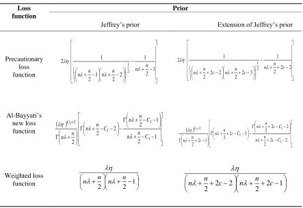
Table 1: Bayes estimator under Jeffrey’s and Extension of Jeffrey`s Priors, using different Loss Functions

Loss function

Prior

Jeffrey’s prior Extension of Jeffrey’s prior

Precautionary loss

function 2

1

2 2 1

2 _

          ₊ ₋     

 ₊ ₋ n

n n

n 

 2 1 3 2 2 2 2

2 _

          ₊ ₊ ₋       ₊ ₊ ₋ c n n c n

n 



Al-Bayyati’s new

loss function _

     ₊ ₋ ₋ 1 2 C1

n n        ₊ ₊ ₋ ₋ 2 2

2 c C1

n n



Weighted loss

function _

     ₊ 2 n n        ₊ ₊ ₋ 1 2 2 c n n 

Table 2: Posterior risks under Jeffrey’s and Extension of Jeffrey`s Priors, using different Loss Functions

Loss function

Prior

Jeffrey’s prior Extension of Jeffrey’s prior

Precautionary

loss

function _

              − + −             ₊ ₋     

 ₊ ₋ 1

2 1 2 2 1 2 1 2 2 1 _n n n n n n                     − + + −             ₊ ₊ ₋     

 ₊ ₊ ₋ 2 2

2 1 3 2 2 2 2 2 1 2 2 1 c n n c n n c n n     Al-Bayyati’s new loss function ( )             − − +       ₊ ₋ ₋  −       ₊ ₋ ₋        +  + 1 2 1 2 2 2 2 1 1 1 2 1 C n n C n n C n n n n C      ( )             − − + +       ₊ ₊ ₋ ₋  −       ₊ ₊ ₋ ₋        ₊ ₊ ₋  + 2 2 2 2 2 2 3 2 2 1 2 2 1 1 1 2 1 C c n n C c n n C c n n c n n C      Weighted loss

function _ +₂__ +₂−1_ n n n

n 

       ₊ ₊ ₋       ₊ ₊ ₋ 1 2 2 2 2 2 c n n c n

n 

(16)

5. Real Life Data

The following real data set is considered for illustration of the proposed methodology. The data below are from an accelerated life test of 59 conductors, failure times are in hours, and there are no censored observations Lawless (2003).

2.997, 4.137, 4.288, 4.531, 4.700, 4.706, 5.009, 5.381, 5.434, 5.459, 5.589, 5.640, 5.807, 5.923, 6.033, 6.071, 6.087, 6.129, 6.352, 6.369, 6.476, 6.492, 6.515, 6.522, 6.538, 6.545, 6.573, 6.725, 6.869, 6.923, 6.948, 6.956, 6.958, 7.024, 7.224, 7.365, 7.398, 7.459, 7.489, 7.495, 7.496, 7.543, 7.683, 7.937, 7.945, 7.974, 8.120, 8.336, 8.532, 8.591, 8.687, 8.799, 9.218, 9.254, 9.289, 9.663, 10.092, 10.491, 11.038

Programs have been developed in R language to obtain the Bayes estimates and posterior risks and are presented in the tables below:

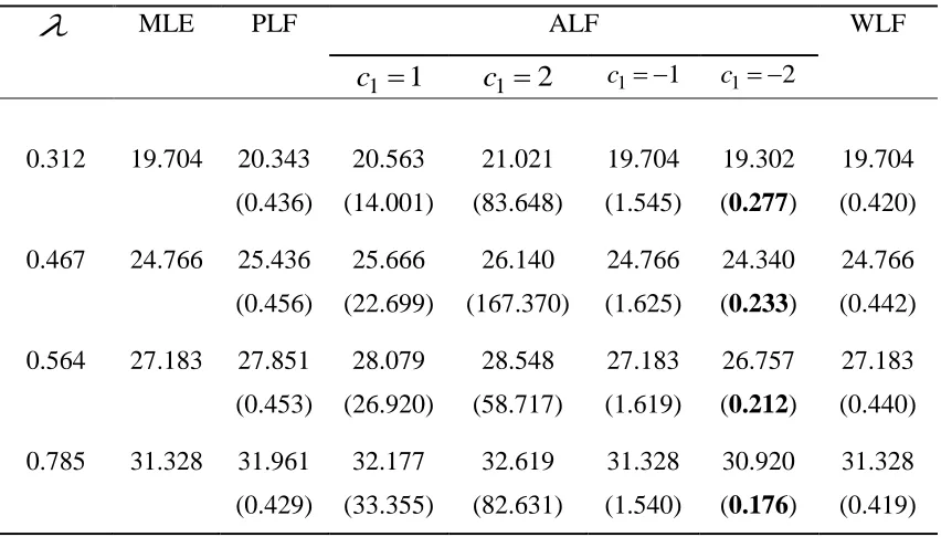
Table 3: Estimates and (Posterior risk) of  under Jeffrey’s prior



MLE PLF ALF WLF

1 1 =

c c₁=2 c₁=−1 c₁=−2

0.312 19.704 20.343

(0.436)

20.563

(14.001)

21.021

(83.648)

19.704

(1.545)

19.302

(0.277)

19.704

(0.420)

0.467 24.766 25.436

(0.456)

25.666

(22.699)

26.140

(167.370)

24.766

(1.625)

24.340

(0.233)

24.766

(0.442)

0.564 27.183 27.851

(0.453)

28.079

(26.920)

28.548

(58.717)

27.183

(1.619)

26.757

(0.212)

27.183

(0.440)

0.785 31.328 31.961

(0.429)

32.177

(33.355)

32.619

(82.631)

31.328

(1.540)

30.920

(0.176)

31.328

(0.419)

(17)

Table 4: Bayes Estimates and (Posterior risk) of  under extension of Jeffrey’s prior



c

PLF ALF WLF

1 1 =

c c₁=2 c₁=−1 c₁ =−2

0.312

0.5 20.343

(0.436)

20.563 (14.001)

21.021 (83.648)

19.704 (1.545)

19.302 (0.277)

19.704 (0.420)

1.0 19.913

(0.418)

20.125 (12.845)

20.563 (74.983)

19.302 (1.482)

18.915 (0.271)

19.302 (0.403)

2.0 19.107

(0.385)

19.302 (10.869)

19.704 (60.697)

18.543 (1.367)

18.186 (0.260)

18.543 (0.371)

2.5 18.728

(0.370)

18.915 (10.023)

19.301 (54.784)

18.186 (1.314)

17.842 (0.256)

18.186 (0.357)

0.467

0.5 25.436

(0.456)

25.666 (22.699)

26.104 (167.379)

24.766 (1.625)

24.340 (0.233)

24.766 (0.442)

1.0 24.986

(0.440)

25.208 (21.122)

25.666 (152.823)

24.340 (1.569)

23.927 (0.229)

24.340 (0.427)

2.0 24.132

(0.410)

24.340 (18.358)

24.766 (127.990)

23.529 (1.466)

23.143 (0.221)

23.529 (0.398)

2.5 23.723

(0.397)

23.927 (17.146)

24.340 (117.415)

23.143 (1.418)

22.770 (0.218)

23.143 (0.385)

0.564

0.5 27.851

(0.453)

28.079 (26.920)

28.548 (58.717)

27.183 (1.619)

26.757 (0.212)

27.183 (0.440)

1.0 27.402

(0.438)

27.623 (25.218)

28.078 (198.918)

26.757 (1.568)

26.344 (0.209)

26.757 (0.426)

2.0 26.550

(0.411)

26.757 (22.200)

27.183 (169.356)

25.944 (1.473)

25.555 (0.203)

25.944 (0.400)

2.5 26.143

(0.399)

26.344 (20.860)

26.757 (156.563)

25.555 (1.429)

25.178 (0.199)

25.555 (0.388)

0.785

0.5 31.961

(0.429)

32.177 (33.355)

32.619 (82.631)

31.328 (1.540)

30.920 (0.176)

31.328 (0.419)

1.0 31.537

(0.417)

31.747 (31.607)

32.177 (77.211)

30.920 (1.500)

30.523 (0.174)

30.920 (0.409)

2.0 30.720

(0.396)

30.920 (28.441)

31.328 (67.597)

30.136 (1.425)

29.758 (0.169)

30.136 (0.387)

2.5 30.327

(0.386)

30.523 (27.007)

30.920 (63.330)

29.758 (1.389)

29.390 (0.167)

(18)

6. Conclusion

In this paper, we define length biased Nakagami distribution and study its various characteristics. The estimates and the posterior risk of the scale parameter of the model have been obtained. The application of the new model has been demonstrated with the help of real life data set. The results are shown in the tables above.

Table 3 and table 4 shows the Bayes estimates and posterior risk of the scale parameter



for different values of the shape parameter



under the Jeffrey’s and extension of Jeffrey’s priors. The initial value of the shape parameter



is obtained through R-software. The value of the loss parameter c₁is taken as ±1 and ±2. We also take different values of the hyper-parameter cas 0.5, 1.0, 2.0, and 2.5 respectively. From both the tables it is clear that as we increase the value of



,

the value of estimates of



increases. The estimates obtained under extension of Jeffrey’s prior coincides with the estimates obtained under Jeffrey’s prior when the value of cis 0.5. It is also observed that as we increase the value of hyper-parameter c,the value of posterior risk decreases. Also the value of posterior risk obtained under extension of Jeffrey’s prior coincides with the values of posterior risk obtained under Jeffrey’s prior when the value of cis 0.5. We also observe that it is the Al-Bayyati’s new loss function which has the minimum value of posterior risk as compared to other loss functions. So we can say that the Al-Bayyati’s new loss function is the better loss function as compared to other loss functions which are compared in this manuscript.

Acknowledgement

The authors extended their sincere thanks and gratitude to the chief editor and referees for the constructive suggestions and comments which greatly helped us in improving the paper.

References

1. Abid A, and Kaveh M. (2000). Performance comparison of three different estimators for the Nakagami m parameter using Monte Carlo simulation. IEEE Communications Letters, 4, 119-121.

2. Ahmad, S.P. and Ahmad, K. (2013). Bayesian Analysis of Weibull Distribution Using R Software. Australian Journal of Basic and Applied Sciences, 7(9), 156-164.

3. Fisher, R.A. (1934). The effects of methods of ascertainment upon the estimation of frequencies. Ann. Eugenics, 6, 13-25.

4. Hoffman, C.W. (1960). The m-distribution, a general formula of intensity of rapid fading. Statistical methods in radio wave propagation: proceedings of a symposium, pergamon press, 3-36.

(19)

7. Lappi, J. and Bailey, R. L. (1987). Forest Science, 33, 725-739.

8. Mudasir, S. and Ahmad, S.P. (2015). Structural properties of length biased Nakagami distribution. International Journal of Modern Mathematical Sciences, 13(3), 217-227.

9. Patil, G.P. & Rao, C.R. (1978). Weighted distributions and size-biased sampling with applications to wildlife populations and human families. Biometrics, 34, 179–184.

10. Rao, C.R. (1965). On discrete distributions arising out of methods of ascertainment, in classical and contagious discrete distributions. G.P. Patil, ed., Pergamon press and statistical publishing society, Calcutta, 320-332.

11. Shanker, K. A. Cervantes, C. Loza-Tavera, H. and Avudainayagam, S. (2005). Chromium toxicity in plants. Environment International, 31, 739-753.

12. Tsui, P., Huang C., and Wang, S. (2006). Use of Nakagami distribution and logarithmic compression in ultrasonic tissue characterization. Journal of Medical and Biological Engineering, 26, 69-73.

13. Varian, H. R. (1975). A Bayesian approach to real estate assessment. Studies in Bayesian econometrics and Statistics in honor of Leonard, J. Savage, (Feigner and Zellner, Eds.) North Holland Amsterdam, 195-208.

14. Yang D. T. and Lin, J. Y. (2000). Food Availability, Entitlement and the Chinese Famine of 1959-61. Economic Journal, 110, 136-58.

15. Zaka, A. and Akhter, A. S. (2014). Bayesian approach in estimation of scale parameter of Nakagami distribution. International Journal of Advanced Science and Technology, 65, 71-80.