www.the-cryosphere.net/8/1105/2014/ doi:10.5194/tc-8-1105-2014
© Author(s) 2014. CC Attribution 3.0 License.
Influence of meter-scale wind-formed features on the variability of
the microwave brightness temperature around Dome C in
Antarctica
G. Picard1,2, A. Royer3, L. Arnaud1,2, and M. Fily1,2
1University Grenoble Alpes, LGGE UMR5183, 38041 Grenoble, France 2CNRS, LGGE UMR5183, 38041 Grenoble, France
3Centre d’Applications et de Recherches en Télédétection (CARTEL), Université de Sherbrooke,
2500 boul. Université, Sherbrooke, Quebec, J1K 2R1, Canada
Correspondence to: G. Picard ([email protected])
Received: 26 June 2013 – Published in The Cryosphere Discuss.: 23 July 2013 Revised: 5 March 2014 – Accepted: 3 May 2014 – Published: 24 June 2014
Abstract. Space-borne passive microwave radiometers are widely used to retrieve information in snowy regions by ex-ploiting the high sensitivity of microwave emission to snow properties. For the Antarctic Plateau, many studies present-ing retrieval algorithms or numerical simulations have as-sumed, explicitly or not, that the subpixel-scale heterogene-ity is negligible and that the retrieved properties were rep-resentative of whole pixels. In this paper, we investigate the spatial variations of brightness temperature over a range of a few kilometers in the Dome C area. Using ground-based ra-diometers towed by a vehicle, we collected brightness tem-perature at 11, 19 and 37 GHz at horizontal and vertical po-larizations along transects with meter resolution. The most remarkable observation was a series of regular undulations of the signal with a significant amplitude reaching 10 K at 37 GHz and a quasi-period of 30–50 m. In contrast, the vari-ability at longer length scales seemed to be weak in the in-vestigated area, and the mean brightness temperature was close to SSM/I and WindSat satellite observations for all the frequencies and polarizations. To establish a link between the snow characteristics and the microwave emission undu-lations, we collected detailed snow grain size and density profiles at two points where opposite extrema of brightness temperature were observed. Numerical simulations with the DMRT-ML microwave emission model revealed that the dif-ference in density in the upper first meter explained most of the brightness temperature variations. In addition, we found that these variations of density near the surface were linked to snow hardness. Patches of hard snow – probably formed by
wind compaction – were clearly visible and covered as much as 39 % of the investigated area. Their brightness tempera-ture was higher than in normal areas. This result implies that the microwave emission measured by satellites over Dome C is more complex than expected and very likely depends on the year-to-year areal proportion of the two different types of snow.
1 Introduction
have a coarse spatial resolution, typically 10–60 km depend-ing on the frequency and the antenna size of the radiome-ter (Colton and Poe, 1999; Kerr et al., 2010). In Antarctic coastal and mountainous regions, the heterogeneity within the radiometer footprint is significant because of the topogra-phy. This limits, for instance, the interpretation of snowmelt events detected by passive microwave data (e.g., van den Broeke et al., 2009). In other regions, and specifically on the flat East Antarctic Plateau, the heterogeneity of the snow-pack is less obvious and its impact on microwave observa-tions is unknown. However, all the applicaobserva-tions cited above presuppose, explicitly or not, that the snow characteristics are spatially homogeneous within the radiometer footprint. This assumption is also required when emission models are run using snow properties measured in one point and results are compared to satellite data (Macelloni et al., 2006; Brucker et al., 2011). Advanced approaches for dealing with the sub-pixel heterogeneity, like unmixing (e.g., Painter et al., 2009), have not yet been considered in Antarctica for passive mi-crowave remote sensing as opposed to other continental sur-faces (Kerr et al., 2012).
The large-scale spatial variations of brightness tempera-ture in Antarctica are well known (e.g., Schneider and Steig, 2002; Fahnestock et al., 2000). The spatial variations of brightness temperature are generally continuous, except in coastal and mountainous regions. Snow properties retrieved from microwave data, like the accumulation (Vaughan et al., 1999; Arthern et al., 2006) or the grain size profile (Brucker et al., 2011), are also spatially continuous. This suggests that the snowpack from one pixel to a neighbor is generally sim-ilar. A particularly homogeneous area was identified on the ice divide near Dome C (Macelloni et al., 2007), which might be suitable for the calibration of passive microwave satellites (Macelloni et al., 2006).
It is, however, evident to most observers in the field that the snow surface is highly variable at the meter and decame-ter scales even on the plateau (Furukawa et al., 1996). Most of the visible features are formed by the erosion and by se-lective deposition of snow resulting from wind and turbu-lence. These wind-formed features include ripples, sastrugi and dunes (Kobayashi and Ishida, 1979). Glazed surfaces (Frezzotti et al., 2002a; Scambos et al., 2012), thermal cracks and irregular patches of hoar on the surface (Gow, 1969; Courville et al., 2007) can also be found at some specific points. These features affect the distribution of snow accu-mulation and represent one of the challenges in scaling up local surface mass balance measurements to the continent scale (Goodwin, 1990; Magand et al., 2008; Das et al., 2013). Although the size of these features is much smaller than the microwave radiometer footprint, they have an influence on the signal. Microwave observations are indeed dependent on the viewing azimuth angle. This is most pronounced for the third and fourth Stokes vector components (Narvekar et al., 2006, 2010). This is weak but detectable for the conventional horizontal and vertical polarizations. For instance, Long and
Drinkwater (2000) found that the variations of brightness temperature due to the viewing azimuth angle are about 2 K rms at Dome C (75◦S, 123◦E) and are as large as 5 K in the
Lambert Glacier basin, which is well above the noise level (<1 K). It is also significant in active remote sensing with altimeters (Remy et al., 2006) and scatterometers (Hyland and Young, 1998; Long and Drinkwater, 2000). In general, the variations are symmetric with respect to the prevailing wind direction (Long and Drinkwater, 2000), which suggests that the wind-formed features visible at the surface or those buried within the snowpack have a significant influence on microwave emission. However, the snow characteristics and wave–matter interactions responsible for the azimuthal de-pendence are unknown.
At intermediate scales – ranging from the scales accessible to observers in the field to the pixel scale – the spatial varia-tions can be observed with high- and moderate-resolution op-tical sensors (e.g., Scambos et al., 2007; Nolin et al., 2002), high-resolution radar (Jezek, 1999) or ground penetrating radar. Notable features include crevasse fields, megadunes (Fahnestock et al., 2000; Frezzotti et al., 2002b), hidden dunes (Anschütz et al., 2006) and emerging features of sub-glacial lakes. These well-known features could, in principle, be masked out in the studies for which the homogeneity of the pixels is critical. This is not the case for the wind-formed features that cover the whole continent and whose areal pro-portion within a pixel might vary over time (Lacroix et al., 2009).
If the sub-pixel heterogeneity had a significant influence on the microwave signal, it would call into question the rep-resentativeness of the parameters retrieved from passive mi-crowave observations in many studies and of the robustness of modeling validation work. Quantifying this influence is therefore important to better understand the relationship be-tween the microwave observations and the snow properties, to improve satellite calibration experiments or retrieval algo-rithms and to combine observations from sensors having dif-ferent spatial resolutions (e.g., passive microwave radiome-ters and altimeradiome-ters).
The objective of this study is to analyze the variability of brightness temperature at subpixel scale around Dome C. To collect the data, we used three ground-based radiometers with a footprint on the order of 1 m operating at a frequency of 11, 19 and 37 GHz. The radiometers were towed by a vehi-cle, thus providing measurements over a few kilometers with a resolution of a few meters. In addition, we collected de-tailed vertical profiles of snow properties at two distinct lo-cations in order to run a microwave emission model and de-termine the properties responsible for the observed variations between the points.
2 Data and study area
A series of ground-based microwave radiometric measure-ments were acquired in January 2012 at Dome C in conjunc-tion with snow property measurements taken in drilled holes up to 8–10 m deep. Temperature profiles recorded hourly near the station were also available.
2.1 Radiometric measurements
Three dual-polarimetric radiometers (Radiometrics©) at 10.67 (hereafter referred to as 11), 19 and 37 GHz were de-ployed on a sledge and used between 25 and 31 January to ac-quire brightness temperature data in an area east of the Con-cordia Station near Dome C (Fig. 1). Two types of measure-ments were acquired: (1) continuous measuremeasure-ments along a series of kilometer-long transects to characterize the spa-tial variations of brightness temperature and (2) angular dia-grams at two specific locations selected for their contrasting conditions.
For the transect measurements, the sledge was towed by a vehicle at moderate speed between 3 and 5 km h−1. The radiometers were continuously operating and provided mea-surements with an integration time of 6 s. With an average speed of 4 km h−1, it corresponded to an along-track hor-izontal resolution of about 7 m. The cross-track resolution depended on the radiometer aperture (about 8◦ for 11 GHz and 6◦for 19 and 37 GHz), radiometer height above ground (about 1.5 m) and the radiometer inclination angle with re-spect to the vertical (referred to as the incidence angle). It was on the order of 60 cm for an incidence angle of 55◦. In
addition, two transects (200–300 m long) were acquired at a slower speed (<1 km h−1), thus providing measurements at a finer horizontal resolution. To determine the repeatability, the A3–A4 transect (see Fig. 1) was repeated three times for three different days at nearly constant incidence angle. The S4–S5 transect was repeated four times with varying inci-dence angles the same day. The position of the vehicle was recorded by GPS every second with an estimated precision better than 5 m (when the vehicle was immobile). The sledge with the radiometers was about 7 m behind the GPS receiver. On the high-resolution transects, the track of the sledge was exactly the same (<10 cm rms) for the successive passes, which was negligible with respect to the GPS localization error.
Static measurements were taken at two locations (called SP1 and SP2; see Fig. 1) where contrasting brightness tem-peratures were noticed along the transects. The angular di-agrams were acquired by recording measurements over at least 3 min for every angle. Since the radiometer position was fixed, the footprint center at the surface was located at 0.4 m from the radiometer vertical for incidence angle of 20◦and 2.5 m for incidence angle of 65◦. The volume from which the radiation emanated was larger than that since the
pene-tration depth was on the order of 0.75 m at 37 GHz and 4 m at 19 GHz (Surdyk, 2002; Picard et al., 2009).
Several experimental issues limited the quality of the data set: microwave radiometers are sensitive instruments that re-quire a stabilized inner temperature at+40◦C. With air tem-perature during the measurements around−37◦C, the sta-bility was challenging. Based on several calibrations with an ambient blackbody, we inferred that absolute accuracy was on the order of 3 K. This value was confirmed by day-to-day variations observed during the repeatability tests and by com-paring data acquired on different dates along the same tran-sect (Sect. 2.2). Nevertheless, the stability of the radiome-ters over daily and shorter terms was much better. For in-stance, during the static measurements, the variations were not greater than 0.1 K rms for at least 3 minutes at all the frequencies and incidence angles.
Another issue is the variation of the inclination of the ra-diometers during the transect measurements. The inclination was not constant owing to sledge movement (rolling) and re-laxation of the radiometer mounting due to vibrations. Based on the incidence angles measured within each radiometer with every brightness temperature acquisition, it was pos-sible to discard the records at angles outside of a specified range (e.g., 50–57◦, the precise values are chosen for each graph; see Sect. 3).
In addition, there was a problem with the electronics of the 37 GHz radiometer, and it only recorded every other mea-surement (i.e., every 12 s). This resulted in a degraded along-track resolution. The 11 GHz radiometer was available only on the site the last 2 days due to logistical constraints. De-spite these issues, the data set showed consistent spatial vari-ations (Sect. 3.1) whose amplitude was much larger than the uncertainties.
0 1000 2000 3000 m
Prevailing winds
Figure 1. Location of the experiment in January 2012. The semi-transparent blue symbols represent the individual measurements. The letter and number labels identify points along the transects used for reference. SP1 and SP2 are the locations where detailed snow property mea-surements were collected to run the DMRT-ML microwave emission model. The green point identifies the location of the snow temperature profile.
2.2 Snow properties
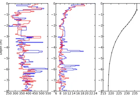
The SP1 and SP2 locations (Fig. 1) where contrasting bright-ness temperatures were noticed were located 400 m apart and differed at first sight by the hardness of the snow: soft (SP1) and very hard (SP2). SP1 also seemed to be about 10–20 cm lower than the surrounding surface while SP2 was located relatively higher. In order to investigate the causes of the spa-tial variations of brightness temperature, we measured pro-files of snow grain size, density and temperature (Fig. 2) nec-essary to run a microwave emission model.
The snow grain size was measured down to 8 m depth us-ing the Profiler Of Snow Specific Surface area Usus-ing short-wave infrared reflectance Measurement (POSSSUM, Arnaud et al., 2011). This instrument measures the reflectance (at 1300 and 805 nm) of the snow face in drilled holes with a centimeter vertical resolution. The reflectances are converted into specific surface area (SSA) using a complex algorithm (Arnaud et al., 2011) that was validated with independent measurements (Gallet et al., 2009). The accuracy was esti-mated to 12 %. The SSA is equivalent to the optical radius (e.g., Grenfell and Warren, 1999; Arnaud et al., 2011) and can be used to run microwave emission models after adapta-tion as described in Sect. 2.3.
The density profiles were measured on snow cores sliced every 5 cm with a miter saw. The height and diameter of each
250 300 350 400 450 500 550 Density (kg m−3)
8 7 6 5 4 3 2 1 0
Depth (m)
6 8 10 1214 16 1820 2224 Specific surface area (m2 kg−1)
8 7 6 5 4 3 2 1 0
215 220 225 230 235 240 Temperature (K) 8
7 6 5 4 3 2 1 0
Figure 2. Density and snow-specific surface area profiles at SP1 (blue, soft snow, low brightness temperature) and SP2 (red, hard snow, high brightness temperature). Temperature profile recorded near the station.
The temperature profile was required for modeling the brightness temperature. With an actual snow accumulation of about 8–10 cm per year at Dome C, the probe installed near the surface in 2006 was at about 50 cm depth in Jan-uary 2012. Even though no temperature data were measured above this depth, we assumed that, during the particular pe-riod of the fieldwork campaign, the temperature was uniform in the uppermost 50 cm. This was supported by the fact that (1) the air and 50 cm temperatures were close and (2) were almost constant during the campaign. Since the temperature profile is governed by diffusion processes, strong tempera-ture gradients could hardly have persisted during this period under these conditions. For modeling, we used the tempera-ture profile averaged over the period.
2.3 DMRT-ML modeling
The Dense Media Radiative Transfer model – Multi Layer (DMRT-ML) predicts the brightness temperature for snow-covered areas from the physical properties of the snowpack. The model is described in detail in Picard et al. (2013) and is available online (http://lgge.osug.fr/~picard/dmrtml/). Each snow layer is fully described by the temperature, density, the radius of the ice spheres representing the snow, and by the amount of liquid water.
The model was evaluated at Dome C (Brucker et al., 2011, B11 hereafter) using similar inputs as used here considering monodisperse nonsticky ice spheres to represent snow. An important result of B11 is that the grain size derived from the SSA – i.e., the radius of the spheres having the same SSA as the snow, r= 3
SSAρice where ρice=917 kg m
−3 – must
be scaled by an empirical factor φ to obtain modeling re-sults in reasonable agreement with the observations (2 K rms over a 2 yr long time series of daily brightness temperature; see B11 for details). The optimal φ value was 2.8 in B11.
160 170 180 190 200 210
TB
(K
) 19V
37V 19H 37H
06 Jan 13 Jan 20 Jan 27 Jan 03 Feb 10 Feb 17 Feb 24 Feb 220
230 240 250 260 270
Temperature (K)
Air Snow (40 cm depth)
Figure 3. Evolution of SSM/I brightness temperatures at 19 and 37 GHz and vertical and horizontal polarizations in January and February 2012. Air temperature measured by the Antarctic Au-tomatic Weather Station Project (AWS) and snow temperature at 50 cm depth. The gray bar shows the period of ground-based radio-metric measurements.
Roy et al. (2013) and Dupont et al. (2014) have confirmed these results using a similar approach with independent data and in different environments, but they have found slightly higher values ofφ. The need to introduceφis probably due to the representation of snow microstructure by monodisperse nonsticky spheres as discussed in Roy et al. (2013).
The method applied here follows B11, with several im-provements: (1) theφfactor was optimized with snow mea-surements and brightness temperature meamea-surements from two different locations (SP1 and SP2) instead of one, and (2) our SSA profiles were 8 m long instead of 3 m in B11. An important consequence was that we did not need the op-timization of a second parameter to represent the mean grain size below the measured profile as used in B11; (3) the snow layers containing more ice than air per volume (i.e., density was larger than 458 kg m−3) were represented by air spheres embedded in an ice background instead of ice spheres in an air background. It yielded a better representation of the medium (Dierking et al., 2012; Picard et al., 2013; Dupont et al., 2014) and extended the validity of the DMRT theory towards large density values.
160 170 180 190 200
T
B(K
)
A3 A4
37 GHz
V-pol Jan 26 (55°) V-pol Jan 27 (54°) V-pol Jan 31 (60°) H-pol Jan 26 (55°) H-pol Jan 27 (54°) H-pol Jan 31 (60°)
160 170 180 190 200
T
B(K
)
A3 A4
19 GHz
V-pol Jan 26 (55°) V-pol Jan 27 (58°) V-pol Jan 31 (60°) H-pol Jan 26 (55°) H-pol Jan 27 (58°) H-pol Jan 31 (60°)
0 50 100 150 200 250
Distance (m)
160 170 180 190 200
T
B(K
)
A3 A4
11 GHz
V-pol Jan 31 (60°) H-pol Jan 31 (60°)
Figure 4. Brightness temperature measured along the A3–A4 transect on different dates (26, 27 and 31 January) for three frequencies (11, 19 and 37 GHz) and nearly constant incidence angle (its mean value along the transect is indicated in the legend). The symbols represent individual measurements at vertical polarization (triangles) and horizontal polarization (squares). The solid curves show the running average for a 6 m window. The horizontal black lines show the mean brightness temperature during the campaign of the pixel containing Dome C from SSM/I (solid line) and WindSat (dashed line).
simplification had a limited impact on the calculated bright-ness temperature since the e-folding penetration depth was about 4 m at 19 GHz and 0.75 m at 37 GHz (Surdyk, 2002; Brucker et al., 2011). The corresponding profiles of SSA, density and temperature are presented in Fig. 2 for both lo-cations.
3 Results
The spatial variations of brightness temperature are analyzed using the two fine-resolution transects. To explain these vari-ations, we present modeling simulations at two locations. The results are generalized using the longer coarse-resolution transects.
3.1 Undulations along two fine-resolution transects The brightness temperatures measured along the A3–A4 transect (see Fig. 1) are shown in Fig. 4 as a function of the distance from A3 towards A4. The individual measurements (squares and triangles) and the smoothed curves (solid lines) show clear undulations. To confirm the reality of these undu-lations, we performed three passes on different days. Except an apparent shift of respectively+6 and−6 m for the second
and third passes, the undulations have similar characteristics for the three passes. The passes corrected from these GPS acquisition error are shown in Fig. 4. At 19 GHz the bright-ness temperatures measured on 31 January are lower than the two other days. Even though the incidence angle was slightly higher and may partially explain this offset, the radiometer stability issue is another probable cause. The linear correla-tions between the passes are larger than 0.70 at 37 GHz and 0.43 at 19 GHz, which is significant (p value<0.01). This confirms that the measurements are reproducible and the un-dulations are real.
160 170 180 190 200
T
B(K
)
S4 S5
37V (60°)
37V (54°)
37V (48°)
37H (60°)
37H (54°)
37H (48°)
160 170 180 190 200
T
B(K
)
S4 S5
19V (58°)
19V (54°)
19V (49°)
19H (58°)
19H (54°)
19H (49°)
Distance (m)
160 170 180 190 200
T
B(K
)
S4 S5
11V (57°)
11V (54°)
11V (49°)
11H (57°)
11H (54°)
11H (49°)
0 50 100 150 200 250
Distance (m)
0.78 0.80 0.82 0.840.86 0.88 0.90 0.92 0.94
Polarization ratio H/V
S4 S5
37 GHz
19 GHz
11 GHz
Figure 5. Brightness temperature (three top plots) and polarization ratio (bottom plot) measured along the S4–S5 transect at three frequencies (11, 19 and 37 GHz) and for various incidence angles. The symbols represent individual measurements at vertical polarization (triangles), horizontal polarization (squares) and polarization ratio (cross). The curves show the running average with a 12 m window. The horizontal black lines show the mean brightness temperature during the campaign of the pixel containing Dome C from SSM/I (solid line) and WindSat (dashed line).
behavior: a decrease from high to low frequencies and from horizontal to vertical polarizations.
Figure 5 shows the brightness temperatures along the sec-ond fine-resolution transect, S4–S5. The different passes were acquired with different incidence angles one after an-other within about an hour. The general characteristics are similar to those of A3–A4. Seven local maximum, separated by a distance of 36 m on average, were found along the S4– S5 transect. The amplitude of the undulations shows the same dependence on the polarization and frequency as found in the previous transect. The incidence angle influences the overall level of the brightness temperatures at horizontal polariza-tion, and at vertical polarization at 19 GHz only. In contrast, the different passes at 37 GHz and vertical polarization are similar, which confirms the good reproducibility of the mea-surements.
Table 1. Mean and standard deviation (in parentheses) of the brightness temperatures for the A3–A4 (at different dates) and S4–S5 (at dif-ference incidence angles) transects; mean brightness temperatures measured by SSM/I and WindSat during the field campaign and corrected for the upwelling atmospheric contribution and the transmission through the atmosphere.
Transect/passes 37 GHz 19 GHz 11 GHz
V-pol H-pol V-pol H-pol V-pol H-pol
Transect A3–A4
25 Jan 195.0 (3.1) 176.7 (4.7) 198.1 (0.6) 174.2 (2.6) n/a n/a
26 Jan 194.8 (3.0) 176.7 (4.0) 197.3 (0.8) 171.7 (3.0) n/a n/a
31 Jan 192.6 (3.1) 175.1 (5.0) 194.4 (0.9) 168.7 (3.2) 198.1 (1.3) 166.0 (3.7)
Transect S4–S5
60◦ 193.5 (3.2) 175.3 (4.2) 195.4 (0.9) 169.0 (2.9) 198.7 (1.0) 166.9 (3.3) 54◦ 193.3 (3.1) 178.7 (4.0) 195.8 (0.8) 170.9 (2.7) 199.4 (1.0) 169.4 (3.5) 48◦ 194.3 (3.2) 182.2 (4.2) 193.7 (0.8) 171.8 (2.4) 198.5 (0.9) 171.6 (2.2) 42◦ 193.2 (2.8) 182.5 (3.2) 192.4 (0.7) 175.6 (1.7) 197.2 (0.9) 174.0 (1.7)
SSM/I 195.6 177.9 197.4 171.7 n/a n/a
WindSat 196.9 179.6 199.6 173.0 199.2 167.0
well. Hence, we conclude that the variations observed in the brightness temperatures and PR are caused by two different electromagnetic mechanisms.
The next Sect. 3.2 seeks the origin of these mechanisms, and the Sect. 3.3 investigates how these results apply at longer length scales.
3.2 Relationship between brightness temperature and snow properties
In order to determine the snow properties responsible for the brightness temperature variations, we used the measure-ments collected at SP1 and SP2 (Fig. 2) to run the DMRT-ML model. We first analyze the radiometric measurements and, second, present the modeling results.
Figure 6 shows the measurements as a function of inci-dence angle at SP1 and SP2 and at 19 and 37 GHz as sym-bols. These measurements present the same characteristic variations in terms of amplitude, frequency and polarization as for the transects A3–A4 and S4–S5. The angular depen-dences have a typical shape (e.g., Tsang and Kong, 2001; Dupont et al., 2014): the vertical polarization reaches a max-imum between 50 and 60◦corresponding to the Brewster an-gle, and it is larger than the horizontal polarization. The hori-zontal polarization decreases with the incidence angle except for large angles for SP2, which could result from the hetero-geneity of the surface and the variations of viewed area as a function of the incidence angle. Visually, the surface at SP2 was indeed more chaotic than at SP1.
The results of the DMRT-ML simulations are shown in Fig. 6 as solid and dashed curves for the vertical and hori-zontal polarizations respectively. These simulations were run with a value ofφ=2.3, a value obtained by manual adjust-ment to get agreeadjust-ment of the mean level between the obser-vations and modeling results considering both frequencies,
20 30 40 50 60 70
Incidence angle (Degree)
150 160 170 180 190 200 210
Brightness temperature (K)
19 GHz 19 GHz
V-pol SP1 H-pol SP1 Obs V-pol SP1 Obs H-pol SP1 V-pol SP2 H-pol SP2 Obs V-pol SP2 Obs H-pol SP2
20 30 40 50 60 70
Incidence angle (Degree) 37 GHz
37 GHz
V-pol SP1 H-pol SP1 Obs V-pol SP1 Obs H-pol SP1 V-pol SP2 H-pol SP2 Obs V-pol SP2 Obs H-pol SP2
Figure 6. Measured and modeled brightness temperature as a func-tion of the incidence angle for two locafunc-tions (SP1 in orange and SP2 in blue), at horizontal (dashed curve and squares) and vertical (solid curve and triangles) polarizations, and at 19 GHz (left) and 37 GHz (right) frequencies.
both locations, and the vertical polarization. Increasingφby 0.1 results in a general decrease of 1.5–2.3 K depending on the angle and location. It means that the optimization of theφ
20
30
40
50
60
70
Incidence angle (Degree)
180
185
190
195
200
205
Brightness temperature (K)
37 GHz
37 GHz
37 GHz
37 GHz
SP1
Obs V-pol SP1
SP2
Obs V-pol SP2
Density from SP1, SSA from SP2
Density from SP2, SSA from SP1
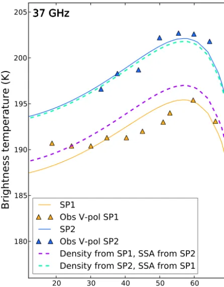
Figure 7. Measured and modeled brightness temperature as a func-tion of the incidence angle for two locafunc-tions at 37 GHz and vertical polarization. Observations and simulations (solid lines) in Fig. 6 are repeated using the same symbols. In addition, simulations with mixed profiles are shown in purple (density from SP1 and SSA from SP2) and cyan (density from SP2 and SSA from SP2).
Table 2. Root mean square error between the modeling results and radiometric measurements at SP1 and SP2.
Frequency Polarization RMSE at SP1 (K) RMSE at SP2 (K)
(GHz) n=10 n=7
19 V 0.9 2.5
19 H 4.5 10.8
37 V 1.5 1.2
37 H 5.2 11.2
The error is quantified using the root mean square (rms) difference between the observations and modeled brightness temperatures over then=10 observations for SP1 orn=7 for SP2. The rms errors reported in Table 2 show that the agreement is, in general, better by a factor of 2 for SP1 than SP2, and better by a factor of around 5 for the vertical than the horizontal polarization. However, the error is relatively independent of the frequency, which indicates that the verti-cal gradient of snow grain size and density is well captured by the measurements (Brucker et al., 2010).
The model reproduces the large difference between SP1 and SP2 at 37 GHz and vertical polarization with an
accu-racy sufficient to investigate the physical cause of the un-dulations observed on the transects. The temperature profile could not be responsible for the difference as it was iden-tical in both simulations. To determine the respective influ-ence of the grain size and density profiles, we ran two other simulations using the density profile of SP1 with the SSA profile of SP2, and vice versa. Figure 7 shows the results at 37 GHz and vertical polarization compared to the origi-nal simulations and the observations. It clearly demonstrates that the exchange of the SSA profiles has a limited impact on the brightness temperature (+1.6 K from orange to pur-ple, and−0.3 K from blue to cyan), whereas swapping the density profiles causes large variations (+6.5 K from orange to cyan, and−5.3 K from blue to purple) with direction and amplitude in agreement with the observations. It means that the density is the main factor explaining the difference in brightness temperature between the two sites. Another simu-lation where only the upper meter of the density profiles was swapped shows very similar results, indicating that the fea-ture responsible for the differences was close to the surface. Density at SP1 and SP2 differs in the upper part of the snow-pack: 390 and 410 kg m−3respectively, on average in the first meter. According to electromagnetic theories (DMRT, Tsang and Kong, 2001, and an improved born approximation, Mät-zler, 1998), a larger density leads to larger absorption and to weaker scattering in snow when the density is in the range of 250–500 kg m−3(Fig. 7; Picard et al., 2013). Both effects combined decrease the single scattering albedo and increase the brightness temperature.
The increase observed at vertical polarization between SP1 and SP2 is also visible at horizontal polarization. At 37 GHz, the brightness temperature increase observed between SP1 and SP2 is larger at horizontal than vertical polarization so that the polarization ratio increases from about 0.89 to 0.92 at 55◦, that is, in the range observed along the transect (Fig. 5). In contrast, at 19 GHz, the polarization ratio remains con-stant at 0.88 between SP1 and SP2. The model predicts a very small difference in the polarization ratio (−0.1 %) from SP1 to SP2, which tends to agree with the observations at 19 GHz but disagrees with those at 37 GHz. This also disagrees with the results along the transects at all the frequencies.
160 170 180 190 200
TB
(K
)
N3 N4 N5 A1 S1 S2 S3 S4 S5 S6 S7 S8
37 GHz
160 170 180 190 200
TB
(K
)
N3 N4 N5 A1 S1 S2 S3 S4 S5 S6 S7 S8
19 GHz
0 2000 4000 6000 8000
Distance (m) 160
170 180 190 200
TB
(K
)
N3 N4 N5 A1 S1 S2 S3 S4 S5 S6 S7 S8
11 GHz
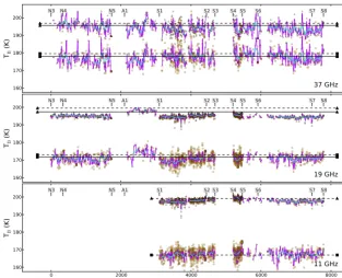
Figure 8. Brightness temperature measured along the N3–N4 (25 January), A1–S1 (26 January) and S1–S8 (31 January) transects for three frequencies (11, 19 and 37 GHz) and nearly constant incidence angles (52 and 57◦). The symbols represent individual measurements at vertical polarization (triangles) and horizontal polarization (squares). The solid curves, violet and blue, show the running average with a box window of 20 and 200 m respectively. The horizontal black lines show the mean brightness temperature during the campaign for the pixel including Dome C from SSM/I (solid line) and WindSat (dashed line).
local slope of the surface and total reflections of emerging radiation, or an indirect effect involving the internal struc-ture of the snowpack (Liang et al., 2009). These mechanisms would be more efficient at grazing angles, which corresponds with the discrepancy in Fig. 6.
Except at high incidence angles for horizontal polariza-tion, the modeling results are accurate enough to conclude that the snow density in the upper meter of the snowpack is the main driver of the variations of brightness temperature between SP1 and SP2.
3.3 Long transects and SSM/I observations
A series of transects totaling nearly 8 km are shown in Fig. 8 covering most of the available transects N3–N4, A1–S1, and S1–S8 (see Fig. 1). The abscissa is the distance along the tra-jectory starting from the northernmost point N3. The curves show the running average with a 20 m (purple) and 200 m (blue) box window.
The undulations could not be identified individually along these transects as it was the case for the A3–A4 and S4–S5 transects. This is probably because of the coarser resolution. According to the sampling theorem (Shannon, 1949), undu-lations should be visible since the spatial resolution (≈7 m at 19 GHz and≈14 m at 37 GHz) was less than half of the typical period of the undulations (≈40 m). The computation of the power spectra using irregular fast Fourier transform
(Greengard and Lee, 2004, results not shown) shows peaks in the range of 30–60 m, but they are not significant. On the other hand, the distance between the undulations observed in Sect. 3.1 is not constant, and the twice coarser resolution at 37 GHz (the most sensitive frequency) prevents detection of undulations.
Although the undulations are not resolved, the signal has some statistical characteristics in common with the fine-resolution transects analyzed in Sect. 3.1: the amplitude of the variations is on the same order (see standard deviations in Table 1), and its dependence on the frequency and polar-ization is very similar – that is, the amplitude is larger at 37 GHz than at the lower frequencies, and it is larger at hor-izontal than at vertical polarization. In addition, most of the variations are concentrated at length scales less than about 100 m. This suggests that the variations observed along the two transects, A3–A4 and S4–S5, are not isolated cases but are representative of the area. Given the large amplitude of these variations, it is important to consider them to under-stand the brightness temperature observed by satellites.
Distance (m)
170175 180 185 190 195 200 205
T
B(K
)
A3 A4
37 GHz
V-pol H-pol
0 50 100 150 200 250
Distance (m) 10
20 30 40 50 60 70
Percent of hard snow
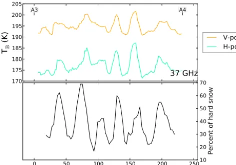
Figure 9. Hardness tested manually along the A3–A4 transect as a function of distance. The penetration in the top 30 cm of the snow-pack was tested using a stick with a 10 mm diameter. The percent of hard snow was calculated by accounting for all these tests in a window (30 m cross-track by 12 m along track) moving along the transect.
acquired at 19 GHz on 26 January along A3–A4 (Fig. 4 and between A1 and S1 in Fig. 8) are systematically greater than the data acquired on 25 and 31 January by about 2.5 K. Nev-ertheless, even considering the uncertainty due to the ex-perimental conditions, we can conclude that the variability decreases with increasing length scales from decameters to kilometers.
The brightness temperatures acquired by satellite, SSM/I (solid line) and WindSat (dashed line), are shown in Figs. 4, 5 and 8. The data correspond to the pixel including Concordia and are the average over the duration of the campaign. The small differences obtained between the two satellites may be due to differences in the sensors (frequency, incidence an-gle), calibration, and/or error due to the geo-spatial projec-tion. Nevertheless, the agreement between the satellite ob-servations and the ground-based radiometer data is close, on average, despite the large difference of spatial resolution and possible uncertainty in the atmospheric correction. It sug-gests that the area that we investigated around Concordia was representative of the whole pixel.
4 Discussion
The variations of brightness temperature along the two fine-resolution transects are significant at 37 GHz (about 10 K) and dominated by undulations separated by about 40 m. It is evident in the field that the maximum brightness temperature is almost systematically found in areas of very hard snow. Indeed, the tip of a pencil (cohesiveness index 4; Fierz et al., 2009) could not penetrate the snow, and the tracks of our vehicle left only traces of the spikes although they entirely sank, about 5 cm deep, everywhere else. Areas of hard snow
were present everywhere along the 8 km of the transects, and we noticed a strong correlation with the maximum bright-ness temperature. Even though the undulations are not di-rectly visible in the microwave data for the coarse-resolution transects (Fig. 8), there is no doubt that the maxima were related to snow hardness.
The snow property measurements collected at SP1 (“nor-mal area”, low brightness temperature) and SP2 (“hard snow area”, high brightness temperature) and the radiative transfer model results (Sect. 3.2) show that the difference in bright-ness temperature is mainly explained by the density in the upper part of the snowpack. The density is indeed higher at SP2, particularly in the top 30 cm (on average 445 kg m−3at SP2 and 375 kg m−3at SP1), which agree with the greater hardness of the snow (even though such a difference is mod-erate with respect to the vertical variability, and hardness and density are not strictly related in general). The density pro-file at SP2 suggests that the vertical extent of the hard snow layer is no more than 50 cm. This was also consistent with our experience in drilling SP2. The horizontal extent was not precisely measured at SP2, but we estimated the emerging part to be about 10 m wide. The measurements for the tran-sect near SP2 (not shown) and for the A3–A4 and S4–S5 transects (Figs. 4 and 5) suggest a larger extent, about 20 m, since the brightness temperature undulations are separated by about 40 m and the shape of the undulation is nearly symmet-ric above and below the mean. It is likely that only a fraction of the hard snow emerges at the surface, and the feature is indeed 20 m wide. These results imply that nearly half of the surface area was hard snow.
Additional measurements along the A3–A4 transect were conducted during the 2012–2013 summer campaign to check this hypothesis. The penetration of a stick (10 mm diameter) into the snowpack was tested every 1 m by six people walk-ing in parallel, at a distance of about 5 m from each other. Two clearly distinct types of snow were found: areas with no hard layer (i.e., the stick penetrated easily up to 30 cm depth) and areas with at least one hard layer between 0 and 30 cm (i.e., the stick was blocked before reaching a depth of 30 cm (hardness below was not tested)). A total of 39 % of the tests indicate hard snow. To refine this, we calculated the percent of hard snow as a function of the distance along the tran-sect with a moving window (12 m along the trantran-sect by 25 m perpendicular to the transect). The result is shown in Fig. 9 along with the brightness temperature at 37 GHz averaged for the three dates (see Fig. 4). The correlation between the mi-crowave signal and the percent of hard snow is remarkable, accounting for possible changes over 1 year, GPS geolocal-ization errors and the subjectiveness of this simple test.
Figure 10. (a) Contour of a “whale back” and (b) longitudinal slice extracted from the same “whale back” in 2006–2007.
of 10–15 m. The thickness was about 50 cm at the center and regularly decreased towards the borders (Fig. 10b). Be-cause of its shape, size and emergence above the mean sur-face, it was called “whale back”. The density was above 500 kg m−3, and the hardness was very high (cohesiveness index 5), which was much higher than the density measured at SP2 in 2012 in the first meter. On the other hand, the SSA was the same as in “normal snow” areas (≈25 m2kg−1). We cannot ascertain whether this particularly regular feature was what caused the variations of brightness temperature every-where. In 2012, there was less evidence of such emerging “whale backs”, and the hard snow area around SP2 seemed irregular. Nevertheless, the general characteristics were sim-ilar.
The formation of the 2012 features was very likely driven by the wind and involved the compaction of small fine grains leading to a highly cohesive wind-packed layer. According to Kobayashi and Ishida (1979), these features could be trans-verse waves (also known as barchan dunes). In fact, the wind speed at Dome C is rarely above the theoretical threshold (15 m s−1; Kobayashi and Ishida, 1979) to form longitudinal dunes. In addition, the contour drawn in 2006 (Fig. 10) was not elongated as in the case of longitudinal dunes. Moreover, in 2012, there was no sign of particular alignments and the brightness temperatures along the A3–A4 and S4–S5 tran-sects show similar variations despite the different orientation with respect to the prevailing wind direction. Specific de-tailed observations of these features are needed in the future to understand their origin. Another key question is whether the areal proportion of these features can significantly change over time. With a difference of about 10 K at 37 GHz between hard and normal snow areas, if the proportion changed by say 10 % over time, the brightness temperature would change by about 1 K.
5 Conclusions
Using ground-based radiometers towed by a vehicle in the area around Dome C in Antarctica, we investigated the spa-tial variability of the brightness temperatures at 11, 19 and 37 GHz for length scales from meters to kilometers. These observations revealed that variations are significant at the meter/decameter scales, especially for the highest frequency. The analysis and the simulations conducted with an elec-tromagnetic model indicate that these variations are mainly caused by the alternation of dense/hard and light/loose snow areas with a quasi-period of 30–50 m. The hard snow areas, representing approximately 40 % of the investigated area in summers 2011–2012 and 2012–2013, seem to be features formed by the wind, that is, dunes or “whale backs”, despite the moderate wind speeds encountered at Dome C.
The study also shows that, for the hectometer to kilometer scales, the variations are much smaller. The average of the ground-based brightness temperature is close to the SSM/I and WindSat satellite observations meaning that the inves-tigated area was representative of the pixel of the satellites including Dome C. An important consequence is that space-borne passive microwave sensors cannot spatially resolve these wind-formed features, but they are very sensitive to the areal proportion of these features. It means that changes in emissivity, like those observed by Lacroix et al. (2009) in the Vostok area, might be solely due to a change in the proportion of these features without significant changes in the properties of the different areas.
program. We acknowledge the Naval Research Laboratory, Naval Center for Space Technology, Washington, DC 20375 USA, which provided the WindSat data through Computational Physics, Inc. (http://www.cpi.com/projects/ws.html). We thank T. Scambos, C. Mätzler and R. Kelly for reviewing this paper.
Edited by: R. Kelly
The publication of this article is financed by CNRS-INSU.
References
Abdalati, W. and Steffen, K.: Passive microwave-derived snow melt regions on the Greenland ice sheet, Geophys. Res. Lett., 22, 787– 790, doi:10.1029/95GL00433, 1995.
Anschütz, H., Eisen, O., Rack, W., and Scheinert, M.: Periodic sur-face features in coastal East Antarctica, Geophys. Res. Lett., 33, L22501, doi:10.1029/2006GL027871, 2006.
Arnaud, L., Picard, G., Champollion, N., Domine, F., Gallet, J., Lefebvre, E., Fily, M., and Barnola, J.: Measurement of vertical profiles of snow specific surface area with a 1 cm resolution us-ing infrared reflectance: instrument description and validation, J. Glaciol., 57, 17–29, doi:10.3189/002214311795306664, 2011. Arthern, R. J., Winebrenner, D. P., and Vaughan, D. G.: Antarctic
snow accumulation mapped using polarization of 4.3-cm wave-length microwave emission, J. Geophys. Res., 111, D06107, doi:10.1029/2004JD005667, 2006.
Brucker, L., Picard, G., and Fily, M.: Snow grain size profiles deduced from microwave snow emissivities in Antarctica, J. Glaciol., 56, 514–526, doi:10.3189/002214310792447806, 2010.
Brucker, L., Picard, G., Arnaud, L., Barnola, J., Schneebeli, M., Brunjail, H., Lefebvre, E., and Fily, M.: Modeling time series of microwave brightness temperature at Dome C, Antarctica, using vertically resolved snow temperature and microstructure mea-surements, J. Glaciol., 57, 171–182, 2011.
Champollion, N., Picard, G., Arnaud, L., Lefebvre, E., and Fily, M.: Hoar crystal development and disappearance at Dome C, Antarctica: observation by near-infrared photography and passive microwave satellite, The Cryosphere, 7, 1247–1262, doi:10.5194/tc-7-1247-2013, 2013.
Chang, W. and Tsang, L.: Conical electromagnetic waves diffrac-tion from sastrugi type surfaces of layered snow dunes on Green-land ice sheets in passive microwave remote sensing, in Proc. IGARSS, 122–125, 2011.
Colton, M. C. and Poe, G. A.: Intersensor calibration of DMSP SSM/I’s: F-8 to F-14, 1987–1997, IEEE T. Geosci. Remote, 37, 418–439, doi:10.1109/36.739079, 1999.
Courville, Z. R., Albert, M. R., Fahnestock, M. A., Cath-les IV, L. M., and Shuman, C. A.: Impacts of an ac-cumulation hiatus on the physical properties of firn at a low-accumulation polar site, J. Geophys. Res., 112, F02030, doi:10.1029/2005JF000429, 2007.
Das, I., Bell, R. E., Scambos, T. A., Wolovick, M., Creyts, T. T., Studinger, M., Frearson, N., Nicolas, J. P., Lenaerts, J. T. M., and van den Broeke, M. R.: Influence of persistent wind scour on the surface mass balance of Antarctica, Nat. Geosci., 6, 367–371, doi:10.1038/ngeo1766, 2013.
Dierking, W., Linow, S., and Rack, W.: Toward a robust re-trieval of snow accumulation over the Antarctic ice sheet using satellite radar, J. Geophys. Res., 117, D09110, doi:10.1029/2011JD017227, 2012.
Dupont, F., Picard, G., Royer, A., Fily, M., Roy, A., and Champol-lion, N.: Modeling the microwave emission of ice; Applications to the Cap Prud’Homme Blue Ice Area in Antarctica and to the Barnes Ice Cap superimposed ice in Arctic, IEEE T. Geosci. Re-mote, 52, 6639–6651, doi:10.1109/TGRS.2014.2299829, 2014. Fahnestock, M. A., Scambos, T. A., Shuman, C. A., Arthern, R. J.,
Winebrenner, D. P., and Kwok, R.: Snow megadune fields on the East Antarctic Plateau: extreme atmosphere-ice interaction, Geo-phys. Res. Lett., 27, 3719–3722, doi:10.1029/1999GL011248, 2000.
Fierz, C., Armstrong, R. L., Durand, Y., Etchevers, P., Greene, E., McClung, D. M., Nishimura, K., Satyawali, P. K., and Sokra-tov, S. A.: The international classification for seasonal snow on the ground, UNESCO/IHP, 2009.
Frezzotti, M., Gandolfi, S., La Marca, F., and Urbini, S.: Snow dunes and glazed surfaces in Antarctica: new field and remote-sensing data, Ann. Glaciol., 34, 81–88, 2002a.
Frezzotti, M., Gandolfi, S., and Urbini, S.: Snow megadunes in Antarctica: sedimentary structure and genesis, J. Geophys. Res., 107, 4344, doi:10.1029/2001JD000673, 2002b.
Furukawa, T., Kamiyama, K., and Station, M. H.: Snow surface fea-tures along the traverse route from the coast to Dome Fuji and Queen Maud Land and Antarctica, in: Proc NIPR Symp. Polar Meteorol. Glaciol., vol. 10, 13–24, 1996.
Gaiser, P., St. Germain, K., Twarog, E., Poe, G., Purdy, W., Richard-son, D., Grossman, W., Jones, W., Spencer, D., Golba, G., Cleve-land, J., Choy, L., Bevilacqua, R., and Chang, P.: The WindSat spaceborne polarimetric microwave radiometer: sensor descrip-tion and early orbit performance, IEEE T. Geosci. Remote, 42, 2347–2361, doi:10.1109/TGRS.2004.836867, 2004.
Gallet, J.-C., Domine, F., Zender, C. S., and Picard, G.: Measument of the specific surface area of snow using infrared re-flectance in an integrating sphere at 1310 and 1550 nm, The Cryosphere, 3, 167–182, doi:10.5194/tc-3-167-2009, 2009. Goodwin, I. D.: Snow accumulation and surface topography in the
katabatic zone of Eastern Wilkes Land, Antarctica, Antarct. Sci., 2, 235–242, doi:10.1017/S0954102090000323, 1990.
Gow, A. J.: On the rates of growth of grains and crystals in south polar firn, J. Glaciol., 8, 241–252, 1969.
Greengard, L. and Lee, J.: Accelerating the nonuni-form fast fourier transnonuni-form, SIAM Rev., 46, 443–454, doi:10.1137/S003614450343200X, 2004.
Grenfell, T. C. and Warren, S. G.: Representation of a nonspherical ice particle by a collection of independent spheres for scatter-ing and absorption of radiation, J. Geophys. Res., 104, 31697– 31710, doi:10.1029/1999JD900496, 1999.
Hyland, G. and Young, N.: Wind-induced directional anisotropy of microwave backscatter and its impact on imaging of the Antarctic continental snow cover, Int. Geosci. Remote Se., 4, 1988–1990, doi:10.1109/IGARSS.1998.703717, 1998.
Jezek, K. C.: Glaciological properties of the Antarctic ice sheet from RADARSAT-1 synthetic aperture radar imagery, Ann. Glaciol., 29, 286–290, doi:10.3189/172756499781820969, 1999. Kerr, Y. H., Waldteufel, P., Wigneron, J.-P., Cabot, F., Boutin, J.,
Escorihuela, M.-J., Font, J., Reul, N., Gruhier, C., Juglea, S., Delwart, S., Drinkwater, M., Hahne, A., Martin-Neira, M., and Mecklenburg, S.: The SMOS mission: new tool for monitoring key elements ofthe global water cycle, P. IEEE, 98, 666–687, doi:10.1109/JPROC.2010.2043032, 2010.
Kerr, Y. H., Waldteufel, P., Richaume, P., Wigneron, J. P., Ferraz-zoli, P., Mahmoodi, A., Al Bitar, A., Cabot, F., Gruhier, C., Ju-glea, S. E., Leroux, D., Mialon, A. and Delwart, S.: The SMOS soil moisture retrieval algorithm, IEEE T. Geosci. Remote, 50, 1384–1403, doi:10.1109/TGRS.2012.2184548, 2012.
Kobayashi, S. and Ishida, T.: Interaction between wind and snow surface, Bound.-Lay. Meteorol., 16, 35–47, doi:10.1007/BF02524396, 1979.
Koenig, L. S., Steig, E. J., Winebrenner, D. P., and Shuman, C. A.: A link between microwave extinction length, firn thermal diffusiv-ity, and accumulation rate in West Antarctica, J. Geophys. Res., 112, F03018, doi:10.1029/2006JF000716, 2007.
Lacroix, P., Legresy, B., Remy, F., Blarel, F., Picard, G., and Brucker, L.: Rapid change of snow surface properties at Vostok, East Antarctica, revealed by altimetry and radiometry, Remote Sens. Environ., 113, 2633–2641, doi:10.1016/j.rse.2009.07.019, 2009.
Liang, D., Xu, P., Tsang, L., Gui, Z., and Chen, K.: Electromag-netic scattering by rough surfaces with large heights and slopes with applications to microwave remote sensing of rough sur-face over layered media, Pr. Electromagn. Res. S., 95, 199–218, doi:10.2528/PIER09071413, 2009.
Liebe, H. : MPM – an atmospheric millimeter-wave prop-agation model, Int. J. Infrared. Milli., 10, 631–650, doi:10.1007/BF01009565, 1989.
Long, D. G. and Drinkwater, M. R.: Azimuth variation in microwave scatterometer and radiometer data over Antarctica, IEEE T. Geosci. Remote, 38, 1857–1870, doi:10.1109/36.851769, 2000.
Macelloni, G., Brogioni, M., and Pampaloni, P.: An experimen-tal campaign in Antarctica for the calibration of low-frequency space-borne radiometers, Int. Geosci. Remote Se., 3980–3983, doi:10.1109/IGARSS.2006.1021, 2006.
Macelloni, G., Brogioni, M., Pampaloni, P., and Cagnati, A.: Multifrequency microwave emission fromthe Dome-C area on the East Antarctic plateau: temporal and spa-tial variability, IEEE T. Geosci. Remote, 45, 2029–2039, doi:10.1109/TGRS.2007.890805, 2007.
Magand, O., Picard, G., Brucker, L., Fily, M., and Genthon, C.: Snow melting bias in microwave mapping of Antarctic snow ac-cumulation, The Cryosphere, 2, 109–115, doi:10.5194/tc-2-109-2008, 2008.
Maslanik, J. and Stroeve, J.: DMSP SSM/I-SSMIS Daily Polar Gridded Brightness Temperatures, Version 4, Boulder, Colorado USA: NASA DAAC at the National Snow and Ice Data Center, 2012.
Mätzler, C.: Improved Born approximation for scattering of radia-tion in a granular medium, J. Appl. Phys., 83, 6111–6117, 1998. Mätzler, C. and Wegmüller, U.: Dielectric properties of freshwater ice at microwave frequencies, J. Phys. D. Appl. Phys., 20, 1623, doi:10.1088/0022-3727/20/12/013, 1987.
Narvekar, P. S., Heygster, G., Jackson, T. J., Bindlish, R., and Li, L.: Azimuthal variations in polarimetric microwave measurements observed over Dome C, Antarctica, in: Society of Photo-Optical Instrumentation Engineers (SPIE) Conference Series, vol. 6410 of Society of Photo-Optical Instrumentation Engineers (SPIE) Conference Series, doi:10.1117/12.693503, 2006.
Narvekar, P. S., Heygster, G., Jackson, T., Bindlish, R., Macel-loni, G., and Notholt, J.: Passive polarimetric microwave sig-natures observed over Antarctica, IEEE T. Geosci. Remote, 48, 1059–1075, doi:10.1109/TGRS.2009.2032295, 2010.
Nolin, A., Fetterer, F., and Scambos, T.: Surface roughness characterizations of sea ice and ice sheets: case studies with MISR data, IEEE T. Geosci. Remote, 40, 1605–1615, doi:10.1109/TGRS.2002.801581, 2002.
Painter, T. H., Rittger, K., McKenzie, C., Slaughter, P., Davis, R. E., and Dozier, J.: Retrieval of subpixel snow covered area, grain size, and albedo from MODIS, Remote Sens. Environ., 113, 868– 879, doi:10.1016/j.rse.2009.01.001, 2009.
Picard, G., Brucker, L., Fily, M., Gallee, H., and Krinner, G.: Mod-eling timeseries of microwave brightness temperature in Antarc-tica, J. Glaciol., 55, 537–551, 2009.
Picard, G., Domine, F., Krinner, G., Arnaud, L., and Lefebvre, E.: Inhibition of the positive snow-albedo feedback by precipita-tion in interior Antarctica, Nature Climate Change, 2, 795–798, doi:10.1038/nclimate1590, 2012.
Picard, G., Brucker, L., Roy, A., Dupont, F., Fily, M., Royer, A., and Harlow, C.: Simulation of the microwave emission of multi-layered snowpacks using the Dense Media Radiative transfer the-ory: the DMRT-ML model, Geosci. Model Dev., 6, 1061–1078, doi:10.5194/gmd-6-1061-2013, 2013.
Remy, F., Legresy, B., and Benveniste, J.: On the az-imuthally anisotropy effects of polarization for altimetric measurements, IEEE T. Geosci. Remote, 44, 3289–3296, doi:10.1109/TGRS.2006.878444, 2006.
Roy, A., Picard, G., Royer, A., Montpetit, B., Dupont, F., Lan-glois, A., Derksen, C., and Champollion, N.: Brightness temper-ature simulations of the Canadian seasonal snowpack driven by measurements of the snow specific surface area, IEEE T. Geosci. Remote, 51, 4692–4704, doi:10.1109/TGRS.2012.2235842, 2013.
Scambos, T. A., Haran, T. M., Fahnestock, M. A., Painter, T. H., and Bohlander, J.: MODIS-based Mosaic of Antarctica (MOA) data sets: continent-wide surface morphology and snow grain size, Remote Sens. Environ., 111, 242–257, 2007.
Scambos, T. A., Frezzotti, M., Haran, T., Bohlander, J., Lenaerts, J., Van Den Broeke, M., Jezek, K., Long, D., Urbini, S., Far-ness, K., Neumann, T., Albert, M., and Winther, J.: Extent of low-accumulation “wind glaze” areas on the East Antarctic plateau: implications for continental ice mass balance, J. Glaciol., 58, 633–647, doi:10.3189/2012JoG11J232, 2012.
Schneider, D. P., Steig, E. J., and Comiso, J. C.: Recent climate vari-ability in Antarctica from satellite-derived temperature data, J. Climate, 17, 1569–1583, 2004.
Shannon, C.: Communication in the presence of noise, P. IRE, 37, 10–21, doi:10.1109/JRPROC.1949.232969, 1949.
Shuman, C. A., Alley, R. B., and Anandakrishnan, S.: Character-ization of a hoar-development episode using SSM/I brightness temperatures in the vicinity of the GISP2 site, Greenland, Ann. Glaciol., 17, 183–188, 1993.
Shuman, C. A., Alley, R. B., Anandakrishnan, S., and Stearns, C. R.: An empirical technique for estimating near-surface air ture trends in central Greenland from SSM/I brightness tempera-tures, Remote Sens. Environ., 51, 245–252, 1995.
Surdyk, S.: Using microwave brightness temperature to detect short-term surface air temperature changes in Antarctica: an an-alytical approach, Remote Sens. Environ., 80, 256–271, 2002.
Torinesi, O., Fily, M., and Genthon, C.: Interannual variability and trend of the Antarctic summer melting period from 20 years of spaceborne microwave data, J. Climate, 16, 1047–1060, 2003. Tsang, L. and Kong, J. A.: Scattering of Electromagnetic Waves,
vol. 3, Advanced Topics, Wiley Interscience, New York, 2001. van den Broeke, M., Konig-Langlo, G., Picard, G., Kuipers M. P.,
and Lenaerts, J.: Surface energy balance, melt and sublimation at Neumayer Station, East Antarctica, Antarct. Sci., 22, 87–96, doi:10.1017/S0954102009990538, 2009.
Vaughan, D. G., Bamber, J. L., Giovinetto, M., Russell, J., and Cooper, A. P. R.: Reassessment of net surface mass balance in Antarctica, J. Climate, 12, 933–946, 1999.