Nonlinear Processes
in Geophysics
c
European Geosciences Union 2003
Cyclic Markov chains with an application to an intermediate
ENSO model
R. A. Pasmanter1and A. Timmermann2
1KNMI, Postbus 201, 3730 AE De Bilt, the Netherlands
2Institut f¨ur Meereskunde, D¨usternbrooker Weg 20, D-24105 Kiel, Germany
Received: 4 September 2001 – Revised: 3 June 2002 – Accepted: 24 June 2002
Abstract. We develop the theory of cyclic Markov chains and apply it to the El Ni˜no-Southern Oscillation (ENSO) pre-dictability problem. At the core of Markov chain modelling is a partition of the state space such that the transition rates between different state space cells can be computed and used most efficiently. We apply a partition technique, which di-vides the state space into multidimensional cells containing an equal number of data points. This partition leads to mathe-matical properties of the transition matrices which can be ex-ploited further such as to establish connections with the dy-namical theory of unstable periodic orbits. We introduce the concept of most and least predictable states. The data basis of our analysis consists of a multicentury-long data set obtained from an intermediate coupled atmosphere-ocean model of the tropical Pacific. This cyclostationary Markov chain ap-proach captures the spring barrier in ENSO predictability and gives insight also into the dependence of ENSO predictabil-ity on the climatic state.
1 Introduction
One of the main challenges being addressed by climate re-search is that of climate prediction on time scales ranging from several months to years and up to decades. In this con-text, modern statistical techniques (e.g. Barnston and Ro-pelewski, 1992; Penland and Magorian, 1993; Xue et al., 1994; van den Dool and Barnston, 1995; Tangang et al., 1997) as well as climate models of different complexity (e.g. Cane et al., 1986; Zebiak and Cane, 1987; Blumen-thal, 1991; Goswami and Shukla, 1991a, b; Balmaseda et al., 1994; Oberhuber et al., 1998; Stockdale et al., 1998; Ji et al., 1998; Mason et al., 1999; Gr¨otzner et al., 1998) are being used in order to predict climate fluctuations sufficiently in ad-vance for societies to take precautionary measures. Probably the most prominent example of this is the El Ni˜no-Southern Correspondence to: A. Timmermann
Oscillation (ENSO) phenomenon which, sometimes, can be predicted with an anticipation longer than six months.
Despite recent success in predicting ENSO using statisti-cal and physistatisti-cal models (Latif et al., 1994) it turned out that, partly due to model-reality mismatches and partly due to ini-tial state errors, the models perform very well in some years whereas they fail in others. Similar to the predictability of low-dimensional nonlinear dynamical systems (Smith et al., 1999), ENSO predictability is state dependent. To account for the state dependence of predictability in ENSO models, singular vector techniques have been employed (Chen et al., 1995; Eckert, 1997; Moore and Kleeman, 1997a, b). The singular vectors represent those states of the system which are associated with the strongest error-growth characteristics. However, by construction, they only capture the linear error growth along piecewise linearized trajectories. Furthermore, the computation of singular vectors in ENSO models requires a linearized version of the model code as well as of its ad-joint. For fully coupled general circulation models (CGCMs) such an approach is not feasible due partly to limited com-puter resources and partly to the fundamental problem of for-mulating adjoint operators of coupled systems with different time scales. In our paper we describe an alternative approach, based on the statistical investigation of model generated time series rather than on manipulating computer code (Eckert, 1997; Chen et al., 1995; Moore and Kleeman, 1997a, b). The statistical technique employed here is based on the estimation of a dynamical equation for probability densities. In contra-position to the singular vector approach, see, e.g. Palmer et al. (1998), this technique is fully nonlinear and is also appli-cable to CGCM simulations. The essential part of the dynam-ical equation is a transition matrix which describes the proba-bility of observing, in one time step, transitions between dif-ferent states. This so-called Markov chain approach was al-ready applied to the ENSO prediction problem by Fraedrich (1988)1. Fraedrich’s results are based on rather short ENSO
time series; his analysis is univariate and it does not take into account the cyclostationarity of the ENSO system, see Fl¨ugel et al. (1999). The present work improves on these aspects by applying the theory of cyclic Markov chains to bivariate data series characterizing ENSO. We point out the analogies be-tween cyclic Markov chains and the Floquet theory of ordi-nary differential equations with periodic coefficients. In this way, e.g. one is able to detect the so-called spring-barrier in ENSO’s predictability.
Moreover, we partition the system’s state space in such a way that each multidimensional cell contains the same num-ber of observations, i.e. the system spends an equal amount of time in each cell. This turns out to be not only an efficient way of using the data and the state space, it also leads to a direct and transparent expression of the dynamics in terms of permutations matrices acting on the discretized state space, i.e. in terms of cycles. As the discretization becomes finer, one expects this cycles expansion to converge into the un-stable periodic orbits (UPOs) expansion of chaotic attrac-tors, see, e.g. P. Cvitanovic (1991) and the references therein. Hence, here one could use the term coarse-grained unstable periodic orbits in order to stress the fact that our discretiza-tion of the state space is not arbitrarily fine. A nice example of UPOs in the ENSO context can be found in Tziperman et al. (1997). In practice, one can construct reliable transition matrices for just a small number, for example three, dynami-cal variables. Therefore, it is of utmost importance to choose the right (three) variables, otherwise the results may be prac-tically irrelevant.
The paper is organized as follows: Sect. 2 gives a brief introduction to the theory of cyclic Markov chains with a special emphasis on the connections with dynamical systems and unstable periodic orbits. Also, the connection between the concept of predictability and a suitably defined entropy production, or information loss rate, is brought to the fore. In Sect. 3 we study the state dependence of ENSO as sim-ulated by an intermediate ENSO model (Zebiak and Cane, 1987). We apply univariate and bivariate Markov chains in order to determine both the least and the most predictable states in this model. Also, the predictability spring barrier is recovered. We conclude in Sect. 4 with a summary and dis-cussion of the technique we applied, of the limitations that may show up in practice and of our main results.
2 Theoretical foundation of cyclic Markov chains
Before venturing into ENSO predictability in coupled mod-els, we briefly describe the theory of Markov chains and dis-cuss how to estimate master equations from data also in the case of cyclostationary systems.
Consider a dynamical system withV degrees of freedom denoted byxα,1 ≤ α ≤ V. The Markov chain descrip-tion of the system is obtained by discretizing time as well as the system’s configuration space. After discretizing the time
Vautard et al., 1990; Nicolis et al., 1997; Egger, 2001) and oceano-graphic (Cencini et al., 1999) contexts.
variablet,the dynamical variables at timet+1 are related to their values at the previous time stept by
xα(t+1)=fα(x(t ), ξ(t ), t ),
where ξ stands for any possible random factors, while the explicit time dependence stands for the non-random external factors. For the sake of illustration and of simplicity, let us assume that
xα(t+1)=fα(x, t )+ξα(t ) (1) where the random terms ξα(t ) are Gaussian, uncorrelated and their variances are
ξα(t )ξβ(t0)=12α(t )δαβδ(t−t0). (2) The case12α(t ) =0 describes a deterministic system. Au-tonomous systems correspond to fα(x(t ), t ) = fα(x(t ))
and12α(t )=12αfor allα.
Even in the purely deterministic case, it makes sense to consider the probability of observing, at timet,the dynami-cal variables having values between sayxand(x+dx). We denote this probability density byp(x, t )withp(x, t ) ≥ 0 andR
p(x, t ) dVx=1.The time evolution of this probability density is expressed then in terms of the so-called Frobenius-Perron (FP) integral operator
p(y, t+1)=
Z
dVxL(y|x, t )p(x, t ).
One always has that L(y|x, t ) ≥ 0 and
R
dVyL(y,x, t )=1. In the case of additive Gaussian noise characterized by Eq. (1) and Eq. (2), the explicit form of the Frobenius-Perron operator is
L(y|x, t ):= √
2π
−V
1−1
·exp −
V
X
α=1
(yα−fα(x, t ))2
212
α(t )
!
, (3)
with 1(t ) = QV
α=11α(t ). For autonomous systems, i.e. L(y|x, t )=L(y|x),one has a stationary probability den-sity2, call itpo(x),which is invariant under the time evolu-tion, i.e.
po(y)=
Z
dVxL(y|x)po(x).
If the system is non-autonomous but its dynamics is periodic in time, i.e.L(y|x, t+T )=L(y|x, t ),whereT is the cor-responding period, then the analogue of the stationary distri-bution will be time-dependent: besides the oscillations with periodT it may also contain (sub)harmonics. The system we shall consider, ENSO, is non-autonomous since its dynamics is modulated by the yearly seasonal cycle .
Next, one partitions the state space into a finite numberC
of cells. We will identify each cell by a Latin subscript. The occupation probability of each cell is,
pi(t ):=
Z
i
dVx p(x, t )≥0, (4)
and satisfies C
X
i=1
pi(t )=1.
Our partial knowledge about the state of the system at timet
is contained inp(t ),we callp(t )either the probability dis-tribution or the state vector.
Finally, one defines the cell-to-cell transition ratesmt(j, i) by
mt(j, i)=−i 1RjdVy RidVxL(y|x, t ),
withi =RidVx.
The dimensionless numbers mt(j, i) are the fraction of times that one observes the system in thej-th cell at time
t+1 when the system was in thei-th cell at timet.The par-tition of initial and final states need not be identical. In the following, we deal always with initial and final partitions that are not (necessarily) identical but have the same number of cellsC.The transition ratesmt(j, i)can be seen then as ele-ments of a nonnegativeC×Cmatrix that we shall denote by mt.The conservation of the total probability takes now the form,
C
X
i=1
mt(i, j )=1, for allj. (5)
This means also that the vector(1,1, . . . ,1,1)is a left eigen-vector of the matricesmtwith eigenvalue 1.Nonnegative ma-trices satisfying (5) are called stochastic mama-trices; they form a semigroup, i.e. the product of two stochastic matrices is a stochastic matrix; the inverse of a stochastic matrix, if it ex-ists, is not necessarily a stochastic matrix. The occupation probability of each cell will evolve according to
pi(t+1)=
C
X
j=1
mt(i, j )pj(t ),
whenever the probability densityp(x, t )and/or the kernel L(y|x, t )is sufficiently constant over the x-cells. More-over, by taking finer partitions with largerC one expects to approximate the real dynamics with higher precision.
Nonnegative matrices and, more specifically, stochastic matrices have been extensively studied, see, e.g. Berman and Plemmons (1979). We recall some of the important proper-ties that they share. The Perron-Frobenius theorem tells us that for any stochastic matrix m,1) there is at least one posi-tive eigenvector with eigenvalue 1,i.e. m·v=vandvi >0 for all 1 ≤ i ≤ C,such an eigenvector is called a Perron vector, 2) all other eigenvalues have absolute values smaller
than or equal to 1 and 3) if m is irreducible3, then the pos-itive right eigenvector is unique. The Perron vector, is then the (unique) stationary distribution,po =v.The stochastic matrices we shall encounter are irreducible and, moreover, all their other eigenvalues have absolute values smaller than 1; such matrices are called primitive. Irreducibility means that there is only one attractor in state space.
As just stated, irreducible stochastic matrices have only one positive eigenvector. This means that all other eigenvec-tors have positive and negative components, moreover, some components may be complex. On the other hand, the state vectorsp(t )describe probability distributions, i.e. their com-ponents are nonnegative at all times,pj(t )≥0,for allj and for allt ≥ 0,as it is ensured by the property (5) satisfied by the transition matrices mt.These two observations make evident that the non-Perron eigenvectors are not probability distributions but deviations away from the stationary distri-bution, i.e. deviations with respect to the Perron vector. Sim-ilarly, complex eigenvectors will always be accompanied by their complex conjugates; the presence of pairs of complex conjugate eigenvalues tells us that the corresponding eigen-vectors do not decay monotonically but that they oscillate in time with a period that equals (2π i) /
ln(argλ)
,when it is measured in units of the time step. In the general case, stochastic matrices are neither symmetric nor normal; on the physical relevance of nonnormal matrices see, e.g. Lorenz (1965) and Trefethen et al. (1993).
In order to avoid unnecessary complications, in the next Subsections we limit the discussion to autonomous systems. The generalization to non-autonomous systems is done in Sect. 2.4.
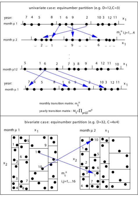
The concept of Markov chains is illustrated and summa-rized in Fig. 1. This figure also shows the main analogies with the expansion of deterministic dynamical systems in terms of eigenvectors of the Frobenius Perron operator. 2.1 Data (equi)partition
Suppose that we are given a long data series consisting ofD
measurements withD 1.We assume that transient phe-nomena (stataistically transient), if present, play a negligible role in the data series. These measurements allow us to de-fine the system state space and subsequently to partition this space into a number of cells. The construction of these cells can be done in an infinite number of different ways. The computation of some important dynamical quantities is sen-sitive to the way in which the cells are constructed. Conse-quently, one is interested in finding those partitions that make reliable and efficient computations possible.
The partitions we have been using are constructed as fol-lows. Consider first the case when one measures only one dynamical variable. Then theD measurements are spread between a minimum and a maximum value; these extreme
3A nonnegative matrix m is irreducible if and only if there is no
permutation P such that PmP†is of the form
S1 0
C S2
month µ 1
month µ 2
year: 7 4 5 8 1 6 9 2 103 1211
1
2 9 6
.. .. .. .. .. .. .. ..
. . .
month µ12
month µ 1
year: 7 4 5 8 1 6 9 2 103 1211
1 2 3 4
5 6 7 8 9 12 11 10
mijµi.j=1,..4
monthly transition matrix: mijµ yearly transition matrix : Mij=Πµ=1,12 mµ
univariate cas e: equinumber partition (e.g. D=12,C =3)
x 1
x2
bivariate cas e: equinumber partition (e.g. D=32, C =4x4)
1
2
3
4 5
6
7
8
9
month µ 1 month µ 2 x 1
x2
x 1
x 1
x 1 x 1
1
2
3
4 5
6
7 1
10
10
1 mijµ
i,j=1,...16
Fig. 1. Data partition for the univariate and bivariate cases.
values define the variable’s range. Partition this range into
Cintervals such that each interval contains an equal number of data points. The number of data points in each interval is
d = D/C.Ideally, we would like to have enough points in each cell so that, potentially, every cell can be accessed from every cell, i.e. one would like to haved ≥C,i.e.D≥C2.
Consider next the two dimensional case, i.e. when one measures two simultaneous dynamical variables. Firstly, par-tition theD data points into
√
C cells along the coordinate corresponding to one of the dynamical variables, each cell containingD/
√
Cpoints4. Then partition each of these cells into
√
Ccells along the second coordinate corresponding to the other measured dynamical variable. In this way one gen-eratesC cells, each one containingd = D/C data points. The procedure is illustrated in Fig. 1.
This partitioning can be applied to higher-dimensional measurements. In this way we can always partition the state space into ‘cells of equal weight’, i.e. the time series spends the same amount of time in each of the cells. It is intuitively clear that this is a very efficient way of defining a partition. This partition does not automatically ensure that the system’s
4For the sake of simplicity, we are assuming that √C and
D/
√
Care integers.
description satisfies the Markovian property. The Markovian property is assumed in our approach and has to be verified a posteriori. Like every sorting procedure, the manipulations required for this task are very time consuming and special algorithms have been developed in order to do this in an ef-ficient way, see, e.g. Chap. 14 of The nature of mathemati-cal modelling by Gershenfeld, Cambridge University Press, (1999) and the references therein.
2.2 Double stochastic matrices and unstable periodic orbits
Since we constructed our partition in such a way that each cell contains the same number of occurrences, it follows that the probability distribution corresponding to the complete data set is represented by the state vector
pdat a=
1/C .. .
1/C
. (6)
Then one must have m·pdat a=pdat a,
i.e.pdat aas given by Eq. (6) is the stationary distribution or Perron vectorpowith eigenvalue 1.This means that, besides the probability conservation constraint (5), the transition ma-trices satisfy also
C
X
k=1
m(i, k)=1. (7)
Non-negative matrices satisfying both constraints (5) and (7) are called doubly stochastic matrices. Also, these matrices form a semigroup.
A theorem by Birkhoff (1946) states a remarkable property of these matrices: every doubly stochasticC×Cmatrix can be written as a convex combination of permutation matrices, i.e.
doubly stochastic M→M=c1P1+ · · · +cNPN (8) withci >0,
N
X
i=1
ci =1 and N ≤C2−2C+2.
the cycles expansion, the Birkhoff expansion is not unique. For example, the Markov chain described by the following doubly stochastic transition matrix,
0 0 1/2 1/2 1/2 1/2 0 0 1/2 1/2 0 0 0 0 1/2 1/2
can be decomposed in terms of permutations in more than one way. One possible decomposition is
1 2
0 0 0 1 1 0 0 0 0 1 0 0 0 0 1 0
+1
2
0 0 1 0 0 1 0 0 1 0 0 0 0 0 0 1
.
Another possible decomposition is:
1 2
0 0 0 1 0 1 0 0 1 0 0 0 0 0 1 0
+1
2
0 0 1 0 1 0 0 0 0 1 0 0 0 0 0 1
.
Generally, one is interested in the expansion (8) with the smallest possible number of termsNand, consequently, with the largest amplitudesci (or longest lifetimes).
In closing this Subsection, it is worthwhile recalling that, for a large class of irreducible stochastic matrices m,it is possible to find positive diagonal matrices D1 and D2 such
that D1·m·D2is a doubly stochastic matrix, see Brualdi et
al. (1966) and Sinkhorn and Knopp (1967). 2.3 Information loss
The transition matrices m may be singular, i.e. one or more eigenvalues may be zero. Evidently, in such a case, some of the information contained inp(t )is irretrievably lost when passing tot +1. More generally, the decay of all modes5 but for the Perron vector, means that information about the departure of the state vectorp(t )from the stationary state
pois lost. How can we quantify this information loss? A convenient and often used measure of the ‘distance’ between, say, a statep(t )andpois6
I (t )= +
C
X
i=1
pi(t )lnp i(t )
pi o
≥0,
This quantity is also bounded from above, lnC ≥I (t ),the maximum value ofI (t )is achieved when only one compo-nent ofp(t )is different from zero. The decay of the modes implies that, on the average, the information contentI (t ) di-minishes7until it reaches zero, i.e. whenpi(t )=poi.
5We use ‘mode’ and ‘eigenvector’ indistinguishably.
6There are other possible definitions; this one is the only exten-sive one, i.e. extenexten-sive over uncorrelated degrees of freedom.
7The decay ofI (t )is not necessarily monotonic: transiently it may happen thatI (t )increases.
Suppose that at t = 0 we know with high precision the state of our system, i.e. att =0 the probability distribution is totally localized in one cell, say it is in cellk,
pi(0)=δik
so that the information attains its maximum possible value
Ik(0)=lnC.One time-step later, the state will bepi(1)=
m(i, k)and the corresponding information content will be
Ik(1)= C
X
i=1
m(i, k)lnm(i, k)+lnC.
Therefore, the information lost in the first time step of the evolution is
1Ik :=Ik(0)−Ik(1)= − C
X
i=1
m(i, k)lnm(i, k)≥0.
By construction, all cells have equal weight (or probability), therefore the probability of starting from cellkis just 1/C.
Averaging over all possible initial conditions, i.e. over all ini-tial cells, we get the average loss of information in one time-step
h1Ii = −1
C
C
X
k=1
C
X
i=1
m(i, k)lnm(i, k)≥0. (9)
Since permutation matrices are characterized bym(i, k) =
δf (k)i for some invertiblef (k)we see that permutation ma-trices achieve the lower bound in information loss. In fact, permutation matrices are the only doubly stochastic matrices withh1Ii = 0. This agrees with our expectations since a permutation corresponds to a totally reversible dynamics.
Notice that the information loss is strongly dependent upon the chosen partition. For example, one can construct the cells in such a contrived way that all the transition rates equal 1/C,i.e.m(i, k)=1/Cfor all(i, j )and the informa-tion loss achieves its largest possible value lnC.On the other hand, the minimum information loss, taken over all possible partitions, is an intrinsic property of the system.
2.4 Cyclic Markov chains and Floquet theory
The effects of the yearly cycle are clearly present in the ENSO phenomenon. In this Subsection we explain how to include this fact in a Markov-chain description.
The data on which the analysis is based are monthly av-erages of some relevant variables. The partition described in the previous Subsections is applied to each month, i.e. we create 12 equipartitions, each with a numberCof cells, each cell containing D/12C number of measurements. This is illustrated in Fig. 1. The precise position in state space of the cells differs from month to month. Next, we compute 12 transition-rate matrices, e.g.m1(i, j )denotes the
yearly cycle starting from month 1 and ending in the same month one year later, is given by
M1:=m12·m11· · · · ·m2·m1
Notice that it is not necessary to compute the twelve in-termediary month-to-month transition matrices mµ in or-der to compute M1, it can be computed directly from the
yearly transition rates, i.e. M1(i, j )is the fraction of
month-1 data points that were in the j-th cell and reached the i -th cell of -the same mon-th one year later. In -this way, it is possible to construct twelve year-to-year transition matrices Mµ, µ=1, . . . ,12.Since the mµare doubly stochastic and irreducible, so are the yearly transition rate matrices Mµ.
In general, the twelve yearly transition matrices Mµwill be different, however, it is easy to show that they have the same eigenvalues{ρn|0≤n≤(C−1)}and that their eigenvectors are simply related. This can be seen as follows: multiply the eigenvalue equation
M1·pn=ρnpn
on the left by the transition matrixm1and obtain
M2·m1·pn=ρnm1·pn
with M2=m1·m12· · · · ·m2.
In other words, m1·pnis an eigenvector of M2corresponding
to the same eigenvalueρn.Similarly, m2·m1·pnis the M3
-eigenvector corresponding toρn.
Being doubly stochastic, all the yearly transition matrices Mµ have the same Perron vector [1,1, . . . ,1] with eigen-valueρ0 = 1.However, recall that the partitions associated with each month are different; consequently, the Perron vec-tor in, e.g. January describes a different probability distri-bution than the, e.g. February Perron vector. In fact, these twelve Perron vectors describe the stationary pdf’s of each month.
The analogy with the classical Floquet theory of ordinary differential equations (1883), see, e.g. Cronin (1980), be-comes evident by introducing a set of matrices Yµ,the ana-logue of Floquet’s fundamental matrix solution, as
Yµ:= [p0µ,p1µ, . . . ,pCµ−1], µ=1, . . . ,12,
where the columnspnµare the eigenvectors of the transition matrix from monthµto the same month one year later, i.e. Mµ·pnµ=ρnpnµwithn=0,1, . . . , C−1,
and the e.g. eigenvalues are, e.g. ordered according to their absolute values,|ρn| ≥ |ρn+1| withρ0 = 1.Our indexµ
corresponds in the Floquet approach to the time modulo the period, in our case, modulo twelve months. Then one has that
Yµ+12=Yµ·8
where8, the analogue of Floquet’s monodromy matrix, is the diagonal matrix[ρ0, ρ1, . . . , ρC−1]and the time-indexµ
is shifted by twelve months, i.e. by one complete cycle.
In the Floquet theory one introduces the monodromy matrix in order to show that it is time-independent; we have already proved that, i.e. that the8as defined above is, indeed, inde-pendent ofµ.
2.5 Reversible and irreversible dynamics
Let us split a doubly stochastic transition matrix M into its symmetric and antisymmetric parts,
Mik =Sik+Aik (10)
Sik = 1
2(Mik+Mki) Aik = 1
2(Mik−Mki) . (11) Due to the doubly stochastic character of M,one has
0≤Sik =Ski≤1, (12)
X
i
Sik=1,
X
k
Sik=1.
In words: the symmetric part of a doubly stochastic matrix is also doubly stochastic. The dynamics generated purely by such a doubly stochastic, symmetric S would consist of decaying, non-oscillating modes, we say that such an S is purely dissipative or diffusive. In mechanics, such a dynam-ics is called irreversible. The matrix elements of the anti-symmetric part A satisfy
−1
2 ≤Aik ≤ 1
2, (13)
X
i
Aik =0, (14)
X
k
Aik =0, (15)
|Aik| ≤Sik. (16)
The dynamics generated purely by the anti-symmetric part A consists of non-decaying, oscillating modes, i.e. A alone would generate a non-dissipative (or conservative) time evo-lution. In mechanics, such a dynamics is called reversible. In the next paragraphs we will discover more reasons for as-sociating A with the conservative part of the dynamics and S with the diffusive part.
The complete dynamics, i.e. the one generated by M=S+A,cannot be obtained by a simple juxtaposition or factorization of the dynamics generated by these two com-ponents separately because, in general, SA 6= AS, conse-quently, the eigenvectors of these matrices will differ.
Let us express the average information loss in terms of the symmetric and anti-symmetric components,
h1Ii = −1
C
C
X
k=1
C
X
i=1
[Sik+Aik] ln [Sik+Aik]
= −1
C
C
X
k=1
C
X
i=1
SiklnSik
1+Aik
Sik
−1
C
C
X
k=1
C
X
i=1
Aikln [Sik+Aik]
= −1
C
C
X
k=1
C
X
i=1
SiklnSik
−1
C
C
X
k=1
C
X
i=1 Sikln
1+Aik
Sik
−1
C
C
X
k=1
C
X
i=1
Aikln [Sik+Aik]. (17)
Therefore, we can writeh1Ii = h1IiS + h1IiA/S where
h1IiSis the information loss that would be generated by the doubly stochastic matrixSexclusively, namely
h1IiS= −1
C
C
X
k=1
C
X
i=1
SiklnSik≥0,
whileh1IiA/Sdepends both on S and A,
h1IiA/S= −1
C
C
X
k=1
C
X
i=1 Sikln
1+Aik
Sik
−1
C
C
X
k=1
C
X
i=1
Aikln [Sik+Aik], (18)
and it vanishes for A=0.Taking into account the antisym-metry of A,one has
h1IiA/S= −1
C
C
X
k=1
C
X
i<k
Sikln
"
1−
Aik
Sik
2#
−1
C
C
X
k=1
C
X
i<k
Aikln
Sik+Aik
Sik−Aik
. (19)
Since|Aik| ≤ Sik, one sees that each term under the first summation sign is negative or zero and that each term under the second summation sign is positive or zero. Moreover, one can check thataln [(s+a) / (s−a)]≥ −sln
1−(a/s)2
for all 0≤s≤1 and|a| ≤s.Therefore,h1IiA/S≤0,i.e. a non-vanishing anti-symmetric component A implies that the entropy production of the doubly stochastic matrix(S+A)
is smaller than that of the doubly stochastic matrix S. The most extreme example of this reduction is provided by the permutations matrices: sinceh1Iipermutation=0 one has that
h1Iipermutation
A/S = − h1Ii
permutation
S <0.
For all these reasons it is natural to associate the anti-symmetric part A with the conservative part of the dynamics. On the other hand, the symmetric part S stems not only from the diffusive part but also from the conservative part of the dynamics, as can be clearly seen in the case of a permutation matrix: a permutation matrix is a purely conservative dynam-ics and yet it has a nonvanishing symmetric part S.One is led to define the purely diffusive components of M asSkl− |Akl| and to measure the overall purely diffusive character of M by
1−C−1P
k,l|Akl|
.
3 Predictability of an intermediate ENSO model
In this section we apply the Markov chain concepts sketched above to data generated by the Zebiak and Cane (ZC) ENSO model (Zebiak and Cane, 1987). The ZC model is a cou-pled atmosphere-ocean model for the tropical region. The atmospheric component consists of a Gill-type, steady-state, linear shallow water model (Gill, 1980) which is formu-lated on an equatorial beta plane. Dissipation is parame-terized in terms of linear Newtonian cooling and Rayleigh friction. Furthermore, a surface-wind parameterization of low-level moisture convergence is used. This model simu-lates reasonably well the steady state atmospheric response to typical sea surface temperature anomalies (SSTA) in the tropics. The ocean model is formulated for a rectangular tropical ocean basin. It is based on a linear, reduced grav-ity model, including a 50 m deep frictional layer, which ac-counts for surface intensification of wind-driven currents. The thermodynamic core of this ocean model takes into ac-count three-dimensional temperature advection by mean and anomalous ocean currents, a linear dependence between sur-face heat flux anomalies and SSTA and the asymmetric effect of vertical advection on temperature. Subsurface temperature anomalies are diagnosed from the variations of the model’s upper layer thickness. The seasonal background fields of sur-face winds and wind divergence, as well as of sea sursur-face temperature are prescribed.
The Zebiak and Cane model generates chaotic ENSO os-cillations in the standard parameter set. As to whether the observations are more adequately described in terms of a stochastically excited damped oscillator (Penland and Sardeshmukh, 1995) or of a chaotic oscillation is an interest-ing issue that has not been solved yet. We do not intend to dwell into the details of this interesting controversy. Small changes in the standard parameters of the ZC model can lead to stable ENSO oscillations, for which noise becomes cru-cial., This sensitivity should be kept in mind when interpret-ing the results of the ZC model. Very often, however, the possibility is ignored that ENSO can be self-sustained dur-ing some decades, whereas it might be stable durdur-ing other decades. In fact there is observational evidence (An and Jin, 2000) that interdecadal background changes in the trop-ical Pacific can trigger changes in the growth rate of ENSO, strong enough to cross the Hopf bifurcation point.
1.2 1.4 1.6 1.8 2 2.2
2 4
6 8
10 12
2 4 6 8 10 12
1 1.5 2 2.5
initialization month entropy production Nino3 S S T A ZC model
lead time [months]
e
n
tr
o
p
y
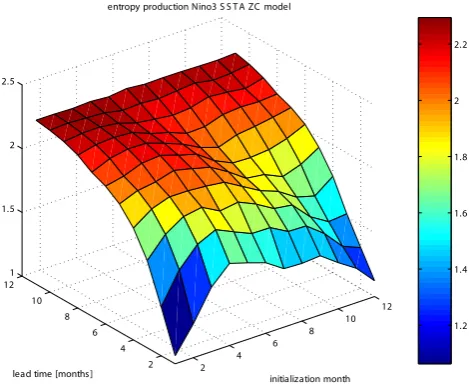
Fig. 2. Seasonal dependence of the entropy production: Entropy as
a function of lead time and of the initialization month.
It is well-known (Balmaseda et al., 1995, Kumar and Hoerling, 1998) that ENSO forecast skills depend on the initial state and in particular, on the season of the year. The so-called predictability barrier characterizes the fact that ENSO predictions initialized in the boreal fall have a sig-nificantly better skill than those initialized in the boreal spring8. This effect might be due to the seasonal changes of ENSO instability related to changing ocean stratification and atmosphere-ocean interactions. As to whether the Ze-biak Cane model is a “realistic” model with respect to sim-ulating the seasonality of the atmosphere-ocean interactions shall not be discussed here9.
We studied this phenomenon by looking at the information loss as a function of lead time and initialization month10.
8Recently Torrence and Webster (2000) introduced the term per-sistence barrier in order account for the fact that the drop of the au-tocorrelation observed during spring (Balmaseda et al., 1995) is not necessarily associated with a complete lack of predictability. Dy-namical ENSO prediction models, however, show that ENSO fore-cast skills are strongly affected by this barrier. In the following, we will thus, use the old term predictability barrier.
9As for the role of the ZC-model, the ZC-model was chosen not because we consider it to be a perfect model for ENSO but just as an illustrative example. The cyclic Markov chain concept can be applied to any kind of ENSO model that yields either stochastically excited linear oscillations or self-sustained chaotic oscillations.
10The transition matrices for a ν-month lead forecast starting from monthµcan be computed as m(ν+µ)=m(ν+µ−1)··m(µ).
However, such a matrix multiplication might increase the rounding errors and this should be avoided in order to ensure that Eq. (5) is satisfied. Hence, we compute the corresponding transition matrix elements, called themmab, directly by counting how many data points in monthµlocated in cellaend up in cellb νmonths later.
−30 −2 −1 0 1 2 3 4
0.5 1
forecasts 1,2,3,...,6 months, initialized in January
−30 −2 −1 0 1 2 3 4
0.5 1
forecasts 1,2,3,...,6 months
−30 −2 −1 0 1 2 3 4
0.5 1
forecasts 1,2,3,...,6 months
Nino3 SSTA [K]
Fig. 3. Initial-state dependence of dispersion in probability space;
the initialization month is January.
3.1 Univariate analysis
Let us first consider an univariate analysis using only the El Ni˜no 3 SSTA index. The computed information loss based on the 640-year long time series for different initialization months and different lead prediction times is shown in Fig. 2. The partition used here isD=640, C =16, d =40 which ensures the accessibility conditionsd ≥CandD≥C2.
One observes that the entropy production quantifying the rate of spread of the probability density is modulated by the annual cycle. More precisely: there is a larger entropy production from March and April and a lower entropy pro-duction for late summer to autumn initialization months; this is the so-called ENSO predictability barrier. One ob-serves furthermore, that for forecasts initialized in, e.g. Au-gust (month 8) the entropy production levels off at a lead time of about six to seven months whereas it increases again for longer lead times. These results are not new but they do illus-trate the utility of cyclic Markov chains in order to quantify predictability.
Notice that in this approach information about the pre-dictability of the system is extracted from one, long, time se-ries and not from a number of simulations initialized on dif-ferent points of the attractor, as is done in ensemble-forecast studies.
In addition to the seasonal cycle effect, the predictability of ENSO might depend also on the state of the tropical Pa-cific itself. This implies that an El Ni˜no forecast starting, e.g. from an El Ni˜no state might have a different quality than a forecast initialized during an intermediate state.
−3 −2 −1 0 1 2 3 0
0.5 1
forecasts 1,2,3,...,6 months, initialized in April
−3 −2 −1 0 1 2 3
0 0.5 1
forecasts 1,2,3,...,6 months, initialized in April
−3 −2 −1 0 1 2 3
0 0.5 1
forecasts 1,2,3,...,6 months, initialized in April
Nino3 SSTA [K]
Fig. 4. Initial-state dependence of dispersion in probability space;
the initialization month is April.
one to strong El Ni˜no conditions. The time evolution for these initial pdfs is shown for lead times from one to six months.
One observes that, starting from strong La Ni˜na condi-tions, upper panel of Fig. 3 the system remains in the La Ni˜na state for about six months. The same holds for strong El Ni˜no conditions, see lower panel of Fig. 3. In contrast to these two large anomaly cases, neutral conditions are much less predictable as can be seen from the fast spread of the pdfs in the middle panel of this Figure. Probably this is a manifes-tation of the fact that under neutral conditions an oscillation exhibits a velocity maximum in state space. This could im-ply that neutral ENSO conditions in January are much more unstable than extreme ENSO conditions.
In Fig. 4 we show the results obtained from the same type of analysis but done now for highly localized initial condi-tions starting in April. We observe qualitatively the same features as for the January initialization case. However, the dispersion rate of the pdfs is much stronger during the boreal spring than during the boreal winter. The main quantitative differences with respect to Fig. 3 can be seen for leads rang-ing from one to three months.
Had we chosen a partition of the state-space into equidis-tant intervals of the index, then the transition rates from and to the extreme-value cells would have been estimated with large errors. Our partition into equal-weight cells has the ad-vantage that the transition rates for the extreme values are estimated as precisely as those for the neutral conditions. On the other hand, a drawback of this partition may be the re-duced physical resolution for extreme ENSO events.
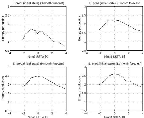
The state dependence of ENSO predictability is summa-rized in Fig. 5. It displays the information loss associated with the El Ni˜no 3 SSTA index for different forecasting lengths. The January initial states are chosen aspi0 = δij, j=1,..., 16.
−4 −2 0 2 4
0.5 1 1.5 2 2.5 3
E pred. (initial state) (3 month forecast)
Nino3 SSTA [K]
Entropy production
−4 −2 0 2 4
0.5 1 1.5 2 2.5 3
E. pred.(initial state) (6 month forecast)
Nino3 SSTA [K]
Entropy production
−4 −2 0 2 4
0.5 1 1.5 2 2.5 3
E. pred.(initial state) (9 month forecast)
Nino3 SSTA [K]
Entropy production
−4 −2 0 2 4
0.5 1 1.5 2 2.5 3
E. pred.(initial state) (12 month forecast)
Nino3 SSTA [K]
Entropy production
Fig. 5. Entropy as a function of the January initial state for
forecast-ing lengths of 3, 6, 9 and 12 months.
In agreement with the previous findings, one observes sat-uration of the entropy production at around a six-month lead and that predictions started from neutral ENSO conditions are less predictable than those initialized during large ENSO events. For a given lead time, we shall call Most Unpre-dictable Modes (MUMs) those initial states that generate the largest information loss and Least Unpredictable Modes (LUMs) those initial states that generate the smallest infor-mation loss. In our analysis we obtain MUMs and LUMS for each month of the year, separately.
In closing this Subsection, let us analyze the eigenmodes of the year-to-year transition matrices Mµ=511i=0mµ+i. As
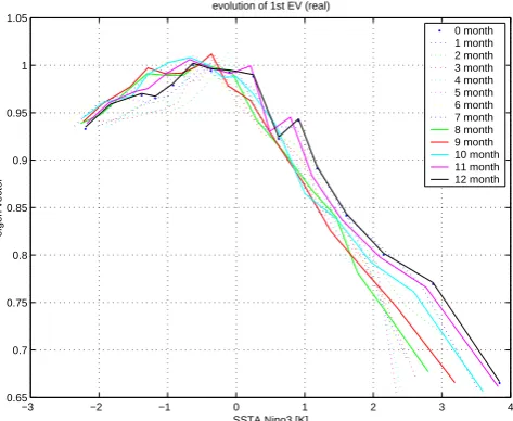
shown in previous sections, all the Mµhave a Perron eigen-vector pµ0 = (1/C, . . . ,1/C),such that Mµ·pµ0 = pµ0. These twelve Perron vectors are nothing else but the aver-age, stationary distributions corresponding to each month. Recalling that each month has its own partition of state space, one realizes that, indeed, the twelve Perron vectors describe different distributions in state space. It is only af-ter a complete twelve-month cycle that we recover the same state space distribution. The distributions corresponding to all twelve Perron vectors have the maximum possible entropy for a partition withCcells, namely, their entropy is lnC. Ac-cordingly, there is no information loss when one starts from this distribution. Another way of stating this is that the Per-ron eigenvector has an infinite lifetime. The time evolution of the Perron vectors starting from the initial month of January is shown in Fig. 6.
We observe that in the first stages of the time evolution the eigenvector of M is rotated away from the El Ni˜no state, whereas the pdf does not change significantly for SSTA val-ues smaller than 2 K. The eigenvector turns back to its origi-nal position after about 7 months.
−3 −2 −1 0 1 2 3 4 0.65
0.7 0.75 0.8 0.85 0.9 0.95 1 1.05
SSTA Nino3 [K]
eigen vector
evolution of 1st EV (real)
0 month 1 month 2 month 3 month 4 month 5 month 6 month 7 month 8 month 9 month 10 month 11 month 12 month
Fig. 6. Time evolution of the leading eigenmode of the yearly
tran-sition matrix M during the course of a year.
that their lifetimes are finite, i.e. that they decay in time. There is another essential difference with respect to the Per-ron vectors, namely, the other eigenvectors are not positive. This reflects the fact that these eigenvectors are not prob-ability distributions but only departures of probprob-ability dis-tributions with respect to the steady distribution, i.e. from the corresponding Perron vector. In meteorological parlance, they are anomalies. Since the matrices Mµ are real, com-plex eigenvalues and their corresponding comcom-plex eigenvec-tors appear always in conjugate pairs; in such a case, the cor-responding departures from the Perron vector do not decay monotically but decay as damped oscillations. There is a connection between these eigenvalues and the periods and lifetimes of the coarse-grained unstable periodic orbits, see, e.g. Cvitanovi´c et al. (1991).
3.2 Bivariate analysis
Next, we present a bivariate study, i.e. Markov chains which are derived from two ENSO-characterizing variables. In the first example, we compute the information loss based on the El Ni˜no 3 SSTA index as generated by the ZC model and the west equatorial thermocline depth anomalies, averaged over the 10◦S–10◦N, 120◦W–180◦W for different initialization months and different lead prediction times. We use Eq. (9) and the cyclostationary transition matrices computed accord-ing to the scheme shown in the lower panel of Fig. 1. The par-tition we use is characterized byD=640, C=16, d =40 which ensures the accessibility conditionsd ≥ CandD ≥
C2. The results are displayed in Fig. 7 where the entropy production has been split into three parts.
– The entropy productionh1Iibased on the full dynam-ics is shown in Fig. 7 upper left panel. Qualitatively and quantitatively we observe very similar features as in the univariate case displayed in Fig. 2. The spring barrier
−4 −2 0 2 4 6
−80 −60 −40 −20 0 20 40
phase space thermocl. depth west, SSTA NINO3
SSTA Nino3 [K]
TDA west [m]
1 1.5 2 2.5
0 5 10 15
0 2 4 6 8 10 12
640 years 16 Cells
1 1.5 2 2.5
0 5 10 15
0 2 4 6 8 10 12
symmetric 640 years 16 Cells
−0.2 −0.15 −0.1 −0.05
0 5 10 15
0 2 4 6 8 10 12
antisymmetric 640 years 16 Cells
Fig. 7. Entropy as a function of lead time and initialization month
as computed for the total (upper left panel), symmetric (lower left panel) and non-dissipative dynamics (lower right panel). A state space view of the SSTA-TDA- trajectory is displayed in the upper right panel.
is retrieved as well as the slowing down of entropy pro-duction after about six months.
– The entropy productionh1IiSdue only to the symmet-ric part of the transition rate matrix is shown in Fig. 7 lower left panel. It can be seen that the total entropy production is mainly dominated by the symmetric part. – The non-dissipative part h1IiA/S which is related to the anti-symmetric part of the transition rate matrix ex-plains only a small part of the information loss. How-ever, a strongly pronounced seasonal modulation of in-formation gain becomes apparent with strongest infor-mation gain to be seen in the boreal summer season. In Fig. 8 we show the one-month lead transition matrix starting in June, its eigenvectors, eigenvalues, and its sym-metric and anti-symsym-metric parts. The eigenvectors are shown in cell-number space. As one can see, also in this case the total transition matrix is dominated by the symmetric part. Hence, even for a one month forecast the dynamics is largely dissipative. The eigenvalue spectrum (Fig. 8f) shows several oscillating modes with frequencies comparable to their decay rates. How these oscillatory modes can be interpreted phys-ically is a question that requires further work. A first step would consist in studying whether they remain unchanged or not when one increases the number of state space cells C.As it is evident, whenC = 16 the longest period that one can detect is 16 months. Similarly, more research should lead to a better understanding of the information contained, e.g. in the asymmetric part of the transition matrices.
0 0.2 0.4 0.6 0.8
5 10 15
2 4 6 8 10 12 14 16
a) trans. matrix 6 1
0 0.2 0.4 0.6 0.8
5 10 15
2 4 6 8 10 12 14 16
b) trans. symmatrix 6 1
−0.2 −0.1 0 0.1 0.2
5 10 15
2 4 6 8 10 12 14 16
c) trans. asymmatrix 6 1
−0.6 −0.4 −0.2 0 0.2 0.4 0.6
5 10 15
2 4 6 8 10 12 14 16
d) real eigenvec.
−0.6 −0.4 −0.2 0 0.2 0.4 0.6
5 10 15
2 4 6 8 10 12 14 16
e) imag eigenvec.
−1 0 1
−0.4 −0.2 0 0.2 0.4 0.6
f) real imag eigenval.
Fig. 8. (a) one month forecast transition matrix starting in June, (b)
its symmetric part, (c) its anti-symmetric part, (d) real part of its eigenvectors, (e) imaginary part of its eigenvectors, (f) its spectrum.
0 0.1 0.2 0.3 0.4
5 10 15
2 4 6 8 10 12 14 16
a) trans. matrix 6 3
0 0.1 0.2 0.3 0.4
5 10 15
2 4 6 8 10 12 14 16
b) trans. symmatrix 6 3
−0.15 −0.1 −0.05 0 0.05 0.1 0.15
5 10 15
2 4 6 8 10 12 14 16
c) trans. asymmatrix 6 3
−0.6 −0.4 −0.2 0 0.2 0.4 0.6
5 10 15
2 4 6 8 10 12 14 16
d) real eigenvec.
−0.6 −0.4 −0.2 0 0.2 0.4 0.6
5 10 15
2 4 6 8 10 12 14 16
e) imag eigenvec.
−1 0 1
−0.4 −0.2 0 0.2 0.4 0.6
f) real imag eigenval.
Fig. 9. (a) transition matrix for a three month forecast initialized
in June, (b) its symmetric part, (c) its anti-symmetric part, (d) real part of its eigenvectors , (e) imaginary part of its eigenvectors, (
¯f) its spectrum.
exactly the same modes, then their spectra would be simply related to each other: the damping factor and the phase of the eigenvalues of the second matrix would be the cubic power and three times those of the one month lead matrix, respec-tively. The associated eigenvectors would show the evolu-tion in state space of the corresponding anomaly. As one can see, the spectra of the two matrices are not so simply related. This is not surprising since there may be more than sixteen modes that dominate the evolution at different phases of the yearly cycle. By increasing the number of cells11 one may detect more dynamically relevant modes, for example, those
11This will require a larger set of data.
140 160 180 200 220 240 260 -15 -10 -5 0 5 10 15 -9 -7 -5 -4 -4 -3 -3 -2 -2 -2 -1 -1 -1 0 0 0 1 1 1 1 1 2 2 2 2 2 3 3 3 3 3 4 4 4 5 5 5 6 6 7
MUM ZC model, 7 month forecast, initialized in January
140 160 180 200 220 240 260 -15 -10 -5 0 5 10 15 -2 -1 -1 -1 0 0 0 0 0 0 1 1 1 1 2 2 2 3 3 3 3
MUM ZC model, 7 month forecast, initialized in May
140 160 180 200 220 240 260 -15 -10 -5 0 5 10 15 -1 -1 0 0 0 0 0 0 1 1 1 1 2 2 2
MUM ZC model, 7 month forecast, initialized in September
with periods longer than 16×3 months=48 months. More-over, as discussed in Sect. 2.2, the transition matrices can be expanded in terms of cyclic permutations that correspond to the coarse-grained unstable periodic orbits of dynamical systems’ theory, Cvitanovi´c et al. (1991). Such a decom-position in terms of UPOs may, in fact, be more revealing than a decomposition in terms of eigenvectors. Again, by en-larging the number of cells, it should be possible to detect more UPOs and to disentangle them better. In this respect, it should be noticed that probably the best way to detect and to disentangle UPOs is to work with three or more dynamical variables, as it is done in Tziperman et al. (1997).
3.3 Most Unpredictable Modes (MUM’s)
It has become quite popular to study similar aspects of error growth in ENSO forecasts (Chen et al., 1995b, Xue et al., 1994, Moore and Kleeman, 1997; Eckert, 1997) due to ini-tial state errors within the linear framework of singular vec-tors (Lorenz, 1965). These vecvec-tors are associated with the fastest linear growth of the initial perturbations due to the non-normality of the tangent linear propagator (Trefethen et al., 1993). They can be computed from the integral propaga-tor of the linearized model. In the case of reduced complex-ity, coupled, atmosphere-ocean models (Chen et al., 1995b; Xue et al., 1994; Moore and Kleeman, 1997; Eckert, 1997) these linearized models and their adjoint can be obtained without facing fundamental difficulties. However, the deter-mination of singular vectors associated with ENSO using a comprehensive CGCM is highly non-trivial and has not been achieved yet. The reason is not only computer power but also the fundamental difference in atmospheric and oceanic time scales. As shown above, the Markov chain approach allows for the extraction of those initial states (or patterns) which are associated with the highest (or the lowest) predictability without any linearization whatsoever. In order to illustrate the type of possible application we have in mind, we have decomposed the simulated thermocline depth field of the ZC model into Empirical Orthogonal functions (EOFs). The two leading EOFs explain about 80% of the variance. These large values of the explained variance are typical for 1 1/2 layer models. We constructed then a Markov chain based on these two leading principal components and searched for those lo-calized initial statesp0j =δij which are characterized by the largest entropy production for a given forecast length. This state is then transformed from cell space back into physical space giving a pair of values for the two principal compo-nents of thermocline depth anomaly which is associated with the largest rate of information loss. Finally, these values of the two principal components are multiplied with their re-spective EOF patterns such as to give an impression of what the initial state which leads to the lowest predictability looks like.
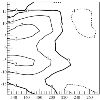
We apply this to three seven-month forecasts, initialized in January, May and September, respectively. The result-ing MUM’s are displayed in Fig. 10. We see that the most unpredictable mode changes during the course of the year.
The MUM computed for a seven-month forecast initialized in January characterizes the discharging of the warm pool. Warm thermocline waters swash the equatorial eastern Pa-cific. This situation is very similar to a situation shortly be-fore a major El Ni˜no event is developed and downwelling Kelvin waves propagate from east to west. The most un-predictable mode for a September forecast has a similar pat-tern to the one initialized during May. MUMs for May and September are characterized by a deep warm pool thermo-cline and a shallow eastern equatorial Pacific. This pattern is dominated mainly by the leading EOF. The MUM for May corresponds to the situation approximately 7 months before a major El Ni˜no event. The warm pool is anomalously deep and short perturbations can lead to the initiation of down-welling Kelvin waves which need about two to three months to cross the Pacific. It is worthwhile noticing that the MUMs computed for different initialization months have very sim-ilar structures to the singular vectors computed for the ZC model, see, e.g. Chen et al. (1995b).
4 Summary and discussion
Our main objective has been to illustrate the capacity and utility of the Markov chain approach in a geophysical con-text, more specifically, in characterizing ENSO and its pre-dictability. To this end, we presented the formalism for cy-clostationary Markov chains and introduced an efficient way of partitioning the state space that also leads directly to an interpretation of the dynamics in terms of coarse-grained un-stable periodic orbits. One of the most attractive aspects of this approach is that it does not require a linear approxima-tion of the dynamics; this stands in contraposiapproxima-tion to the sin-gular vector approach. Another attractive aspect is that the analysis is based on one long, experimental or numerically generated, data series; this should be compared with ensem-ble forecasting which requires numerous numerical simula-tions. Among the straightforward applications presented in Sect. 3, is the identification of the physical configuration that leads to the largest (alternatively, the smallest) uncertainty in predictions with a predefined forecast lead; these states are identified separately for each month. A more standard application is the detection of the spring predictability bar-rier and, less standard, its quantification. It should be noted that the partition into equal weight cells implies that the cells corresponding to the most unprobable observations12occupy a relatively large interval of the variable’s physical range. Sometimes, this may be undesirable.
Needless to say, in order to be able to predict, a good knowledge of the system’s past behaviour is required; this is an inescapable fact that all practical forecasting techniques have to face. In the context of the present article, this means that 1) sufficiently long data series are required in order to be able to make accurate and interesting predictions and 2) the
records should be of more than one relevant dynamical vari-able. Moreover, the choice of these variables is crucial, e.g. if two variables are strongly correlated then one of them is nearly redundant and should be ignored. These two require-ments have been satisfied in, e.g. Tziperman et al. (1997).
Another important question that must be addressed is the so-called Markovian assumption that lays behind the Markov chain approach. The Markovian assumption or Markovian approximation consists in assuming that p(x, t +1), the probability at time step t + 1, is completely determined byp(x, t ), the probability at the previous time stept. No-tice that this is more general than a Markov chain, i.e. the ‘Markovian models’ often found in the literature are not nec-essarily Markov chains. In practice, the Markovian assump-tion is often violated because the set of variablesx that one uses is usually (much) smaller than the total number of rele-vant variables. Whether the Markovian assumption holds or not can be checked a posteriori, e.g. by computing correla-tion funccorrela-tions and comparing them with the corresponding correlation functions in the original data. In many cases one will find that the real system shows stronger, longer lived correlation functions than the Markov chain model does. In principle, the violations of the Markovian approximation can be eliminated by refining the partition and/or by enlarging the setxof dynamical variables, e.g. by including past val-ues of the dynamical variables, etc. In practice, this is hardly feasible.
These comments on the validity of the Markovian approx-imation have important implications for some of the results we have obtained. In particular, it should be clear that some results are no more than lower bounds to predictability. In its turn, this has implications for the development of sophisti-cated physical models: the effort needed in order to develop physical, accurate dynamical models can be justified only if the predictions obtained from such models have a lower un-certainty than the ones obtained from Markov chain models like the one presented in this article.
Our future work will be devoted to the application of cyclic Markov chains to ENSO data obtained from long CGCM simulations. It is our goal to identify those patterns which are associated with least and highest predictability. Furthermore, we plan to study the time evolution of CGCM ENSO pre-dictability more in detail. This can be achieved by projecting the physical fields onto the MUMs and LUMs. The result-ing timeseries quantify how simulated ENSO predictability is modulated in time. Maybe it is possible to attribute phys-ical meaning to these predictability timeseries, such as es-tablishing that, e.g. if the thermocline is anomalously deep for several decades then we might expect better intrinsic pre-dictability of the ENSO system as compared to eras with rel-atively shallow thermocline. This will eventually lead to the generation of probabilistic physical ENSO models.
Acknowledgements. RAP thanks A. Knauf (Erlangen University)
and H. Voss (Freiburg University) for very stimulating conversa-tions. This work was partly sponsored by the German Science Foundation (DFG), partly by the EU project SINTEX ENV4-CT98– 0714.
References
An, S.-I. and Jin, F.-F.: An eigenanalysis of the interdecadal changes in the structure and frequency of ENSO mode, Geophys. Res. Lett., 27, 2573–2576, 2000.
Balmaseda, M. A., Anderson, D. L. T., and Davey, M. K.: ENSO prediction using a dynamical ocean model coupled to statistical atmospheres, Tellus, 46 A, 497–511, 1994.
Balmaseda, M. A., Davey, M. K., and Anderson, D. L. T.: Decadal and seasonal dependence of ENSO prediction skill, J. Climate, 8, 2705–2715, 1995.
Barnston, A. G. and Ropelewski, C. F.: Prediction of ENSO episodes using canonical correlation analysis, J. Climate, 5, 1316–1345, 1992.
Berman, A. and Plemmons, R. J.: Nonnegative matrices in the mathematical sciences, Academic Press, 1979.
Birkhoff, G.: Tres observaciones sobre el algebra lineal, Rev. Univ. Nac. Tucum´an, Ser. A, 5, 147–150, 1946 .
Brualdi, R. A., Parter, S. V., and Schneider, H.: The diagonal equiv-alence of a nonnegative matrix to a stochastic matrix., J. Math. Anal., Appl., 16, 31–50, 1966.
Cane, M. A., Zebiak, S. E., and Dolan, S. C.: Experimental fore-casts of El Ni˜no, Nature, 321, 827–832, 1986.
Cencini, M., Lacorata, G., Vulpiani, A., and Zambianchi, E.: Mix-ing in a meanderMix-ing jet: A Markovian Approximation, J. Phys. Oceanogr., 29, 2578–2593, 1999.
Chen, D., Zebiak, S. E., Busalacchi, A. J., and Cane, M. A.: An improved procedure for El Ni˜no forecasting, Science, 269, 1699– 1702, 1995a.
Chen, Y-Q., Battisti, D. S., Palmer, T. N., Barsugli, J., and Sarachik, E. S.: A study of the predictability oftropical Pacific SST in a coupled atmosphere/ocean model using singular vector analysis: the role of the annual cycle and the ENSO cycle, Mon. Wea. Rev., 125, 831–845, 1995b.
Cronin, J.: Differential equations, Marcel Dekker, New York, 1980. Cvitanovi´c, P.: Periodic orbits as the skeleton of classical and
quan-tum chaos, Physica D, 51, 138, 1991.
Eckert, C.: PhD Dissertation, University of Hamburg, 1997. Egger, J.: Master equations for climatic parameter sets, submitted,
2000.
Fl¨ugel, M. and Chang, P.: Does the predictability of ENSO depend on the seasonal cycle? J. Atmosph. Sciences, 55, 3230–3243, 1998.
Fraedrich, K.: El Ni˜no-Southern Oscillation predictability, Mon. Wea. Rev., 116, 1001–1012, 1988.
Gill. A.: Some simple solutions for heat induced tropical circula-tion, Q. J. R. Meteor. Soc., 106, 447–462, 1980.
Goswami, B. and Shukla, J.: Predictability of a coupled ocean-atmosphere model, J. Climate, 4, 3–22, 1991a.
Goswami, B. and Shukla, J.: Predictability and variability of a coupled ocean-atmosphere model, J. Marine. Sys., 1, 217–228, 1991b.
Gr¨otzner, A., Latif, M., Timmermann, A., and Voss, R.: Interannual to decadal predictability in a coupled ocean-atmosphere general circulation model, J. Climate, 12, 2607–2624, 1998.
Ji, M., Behringer, D. W., and Leetmaa, A.: An improved coupled model for ENSO prediction and implications for ocean initial-ization, Part II: The coupled model, Mon. Wea. Rev., 126, 1022– 1034, 1998.
Kumar, A. and Hoerling, M. P.: Annual cycle of
Latif, M., Barnett, T. P., Cane, M. A., Fl¨ugel, M., Graham, N. E., von Storch, H., Xu, J.-S., and Zebiak, S. E.: A review of ENSO prediction studies, Climate Dynamics, 9, 167–179, 1994. Lorenz, E. N.: A study of the predictability of a 28-variable
atmo-spheric model, Tellus, 17, 321–333, 1965.
Mason, S. J., Goddard, L., Graham, N. E., Yulaeva, E., Sun, L., and Arkin, P. A.: The IRI seasonal climate prediction system and the 1997/8 El Ni˜no event, Bull. Am. Met. Soc., 80, 1853–1873, 1999.
Mo, R. and Straus, D. M.: Probability forecasts for seasonal aver-age anomalies based on GCM ensemble means, COLA Technical Report No. 74, 33, 1999.
Moore, A. M. and Kleeman, R.: The singular vectors of a coupled atmosphere-ocean model of ENSO, I: Thermodynamics, ener-getics and error growth, Quart. J. Roy. Met. Soc., 123, 953–981, 1997a.
Moore, A. M. and Kleeman, R.: The singular vectors of a coupled atmosphere-ocean model of ENSO, II: Sensitivity studies and dy-namical interpretation, Quart. J. Roy. Met. Soc., 123, 983–1006, 1997b.
Nicolis, C., Ebeling, W., and Baraldi, C.: Markov processes, dy-namic entropies and statistical prediction of mesoscale weather regimes, Tellus, 49 A, 108–118, 1997.
Oberhuber, J. M., Roeckner, E., Christoph, M., Esch, M., and Latif, M.: Predicting the 1997 El Ni˜no Even with a global cli-mate model, Geophys. Res. Lett., 13, 2273–2276, 1998. Palmer, T. N., Gelaro, R., Barkmeijer, J., and Buizza, R.: Singular
vectors, metrics and adaptive observations, J. Atmos. Sci., 55, 633–653, 1998.
Penland, C. and Magorian, T.: Prediction of Ni˜no 3 sea surface tem-perature using linear inverse modeling, J. Climate, 6, 1067–1076, 1993.
Penland, C. and Sardeshmukh, P. D.: The optimal growth of tropi-cal sea surface temperature anomalies, J. Climate, 8, 1999–2024, 1995.
Sinkhorn, R. and Knopp, P.: Concerning nonnegative matrices and doubly stochastic matrices, Pacific J. Math., 21, 343–348, 1967.
Smith, L. A., Ziehmann, C., and Fraedrich, K.: Uncertainty dynam-ics and predictability in chaotic systems, Q. J. R. Meteor. Soc., 2855–2886, 1999.
Spekat, A., Heller-Schulze, B., and Lutz, M.: “Grosswetter” circu-lation analysed by means of Markov chains, Meteorol. Rdsch., 36, 243–248, 1983.
Stockdale, T. N., Anderson, D. L. T., Alves, J. O. S., and Bal-maseda, M. A.: Global seasonal rainfall forecasts using a cou-pled ocean-atmosphere model, Nature, 392, 370–373, 1998. de Swart, H. E. and Grasman, J.: Effect of stochastic perturbations
on a low order spectral model of theatmospheric circulation, Tel-lus, 39 A, 10–24, 1987.
Tangang, F. T., Hsieh, W. W., and Tang, B.: Forecasting the equa-torial Pacific sea surface temperatures byneural network models, Climate Dynamics, 13, 135–147, 1997.
Torrence, C. and Webster, P. J.: The annual cycle of persistence in the El Ni˜no-Southern oscillation, Quart. J. Roy. Meteor. Soc., 124, 1985–2004. 2000.
Trefethen, L. N., Trefethen, A. E, Reddy, S. C., and Driscoll, T. A.: Hydrodynamic stability without eigenvalues, Science, 261, 578– 584, 1993.
Tziperman, E., Scher, H., Zebiak, S. E., and Cane, M. A.: Control-ling spatiotemporal chaos in a realistic El Ni˜no prediction model, Phys. Rev. Lett., 79, 1034–1038, 1997.
van den Dool, H. M. and Barnston, A. G.: Forecasts of global sea surface temperature out to a year using the constructed analogue method, Proceedings of the 19th Annual Climate Diagnostics Workshop, Nov. 14–18, 1994, College Park, Maryland, 416–419, 1995.
Vautard, R., Mo, K., and Ghil, M.: Statistical significance test for transition matrices of atmospheric Markov chains, J. Atmosph. Sc., 47, 1926–1931, 1990.
Xue, Y., Cane, M. A., Zebiak, S. E., and Blumenthal, M. B.: On the prediction of ENSO: a study with a low-order Markov model, Tellus, 46 A, 512–528, 1994.