www.atmos-meas-tech.net/8/5113/2015/ doi:10.5194/amt-8-5113-2015
© Author(s) 2015. CC Attribution 3.0 License.
A wide field-of-view imaging DOAS instrument for two-dimensional
trace gas mapping from aircraft
A. Schönhardt1, P. Altube1,2, K. Gerilowski1, S. Krautwurst1, J. Hartmann3, A. C. Meier1, A. Richter1, and J. P. Burrows1
1Institute of Environmental Physics, University of Bremen, Germany 2Dept. of Astronomy and Meteorology, University of Barcelona, Spain 3Alfred-Wegener-Institute (AWI) Bremerhaven, Germany
Correspondence to: A. Schönhardt ([email protected])
Received: 22 December 2013 – Published in Atmos. Meas. Tech. Discuss.: 8 April 2014 Revised: 31 October 2015 – Accepted: 8 November 2015 – Published: 9 December 2015
Abstract. The Airborne imaging differential optical absorp-tion spectroscopy (DOAS) instrument for Measurements of Atmospheric Pollution (AirMAP) has been developed for the purpose of trace gas measurements and pollution mapping. The instrument has been characterized and successfully op-erated from aircraft. Nitrogen dioxide (NO2) columns were retrieved from the AirMAP observations. A major benefit of the push-broom imaging instrument is the spatially contin-uous, gap-free measurement sequence independent of flight altitude, a valuable characteristic for mapping purposes. This is made possible by the use of a charge coupled device (CCD) frame-transfer detector. A broad field of view across track of around 48◦is achieved with wide-angle entrance optics. This leads to a swath width of about the same size as the flight altitude. The use of fibre coupled light intake optics with sorted light fibres allows flexible instrument positioning within the aircraft and retains the very good imaging capa-bilities. The measurements yield ground spatial resolutions below 100 m depending on flight altitude. The number of viewing directions is chosen from a maximum of 35 indi-vidual viewing directions (lines of sight, LOS) represented by 35 individual fibres. The selection is adapted to each sit-uation by averaging according to signal-to-noise or spatial resolution requirements. Observations at 30 m spatial reso-lution are obtained when flying at 1000 m altitude and mak-ing use of all 35 viewmak-ing directions. This makes the instru-ment a suitable tool for mapping trace gas point sources and small-scale variability. The position and aircraft attitude are taken into account for accurate spatial mapping using the Attitude and Heading Reference System of the aircraft. A
first demonstration mission using AirMAP was undertaken in June 2011. AirMAP was operated on the AWI Polar-5 aircraft in the framework of the AIRMETH-2011 campaign. During a flight above a medium-sized coal-fired power plant in north-west Germany, AirMAP clearly detected the emis-sion plume downwind from the exhaust stack, with NO2 ver-tical columns around 2×10¹⁶molecules cm−2in the plume centre. NOxemissions estimated from the AirMAP observa-tions are consistent with reports in the European Pollutant Release and Transfer Register. Strong spatial gradients and variability in NO2amounts across and along flight direction are observed, and small-scale enhancements of NO2above a motorway are detected.
1 Introduction
and a greenhouse gas. The main sources of NOx, apart from natural processes such as lightning, natural biomass burning events and soil emissions, are anthropogenic activities such as fossil fuel combustion by power plants, industry and traf-fic. The spatial and temporal variability of NO2may be large due to variable and small-scale sources, the high reactivity of NOxand a short atmospheric NO2lifetime.
Since the 1970s, atmospheric NO2 amounts have been measured spectroscopically from the ground (Brewer et al., 1973; Noxon, 1975). A powerful and well-established method for the detection of atmospheric trace gases is the dif-ferential optical absorption spectroscopy (DOAS) technique (Platt and Perner, 1980; Platt and Stutz, 2008). Using the passive remote sensing DOAS method, the vertical column integrated amount of a trace gas can be determined from dif-ferent platforms. Our knowledge about global distributions and temporal variation of NO2 has been increased by satel-lite observations from space (e.g. Burrows et al., 1999b; Leue et al., 2001; Richter and Burrows, 2002; Beirle et al., 2003; Richter et al., 2005; Bucsela et al., 2006; Hilboll et al., 2013) which provide valuable long-term and global data sets. Up to the present, spatial variability or point source emissions at spatial scales much below the order of several tens of kilome-tres, however, are not individually resolved from space-based measurements.
The ground-based DOAS technique has been further de-veloped into the widely used MAX-DOAS (multiple axis DOAS) method, utilizing measurements at multiple elevation angles (Hönninger et al., 2004; Wittrock et al., 2004). These measurements provide information on the vertical trace gas profile. In addition to stationary set-ups, DOAS and MAX-DOAS instruments have been used from ships (e.g. Peters et al., 2012), driving cars (Ibrahim et al., 2010) and air-borne platforms. For example, DOAS measurements from high-altitude balloons yield NO2columns and vertical pro-files in the stratosphere (Pfeilsticker and Platt, 1994), and observations from aircraft yield tropospheric NO2amounts over emission point sources and polluted regions (Melamed et al., 2003; Wang et al., 2005), as well as from shipping emissions (Berg et al., 2012). Such airborne measurements are also valuable for satellite validation (Heue et al., 2005). Observing in flight direction, Merlaud et al. (2012) apply a DOAS instrument on an ultralight aircraft and achieve high sensitivity for boundary layer NO2. Utilizing regular flights of an airliner, the CARIBIC project comprises DOAS mea-surements of several trace gases (Dix et al., 2009; Heue et al., 2011). The combination of multiple elevation angles in flight direction has enabled tropospheric NO2profile re-trievals from aircraft (Bruns et al., 2004, 2006). As a further development, Baidar et al. (2013) use a scanning unit as well as motion compensation for accurate selection of the desired elevation angles, with which they retrieve vertical profiles of trace gases and aerosols.
The extension of a DOAS instrument with one viewing di-rection at a time to an imaging design allows simultaneous
observation in multiple independent directions within a large field of view. Imaging DOAS measurements have been per-formed from the ground (Lohberger et al., 2004; Bobrowski et al., 2006) and are regularly performed by the space-borne OMI (Ozone Monitoring Instrument) sensor (Levelt et al., 2006).
Two instrument applications of imaging DOAS from air-craft have already been reported which are based on two con-siderably different instrumental systems. Heue et al. (2008) report on the first imaging DOAS measurements from air-craft observing large-scale NO2 emissions over the South African Highveld power plants. The instrument is based on a commercial grating spectrometer as in the present study. Popp et al. (2012) use the APEX hyperspectral imaging spec-trometer for successful NO2observations over a city. That in-strument has been developed within a broad ESA programme since 1993 and built by an industrial consortium. First data became available in 2008 (Itten et al., 2008).
Recently, the new imaging instrument, HAIDI (Heidelberg Airborne Imaging DOAS Instrument), has been reported, which has been successfully applied to measurements of NO2, SO2, BrO and OClO from anthropogenic emissions, in Polar regions and within volcanic plumes (General et al., 2014, 2015). The HAIDI consists of three DOAS instruments which point in different directions and are used either in whisk-broom or push-broom mode (Schowengerdt, 2007). Observations yield spatial trace gas distributions at ground resolutions below 100 m depending on flight altitude, as well as information on the vertical distribution.
The present study introduces the push-broom Airborne imaging DOAS instrument for Measurements of Atmo-spheric Pollution (AirMAP), which is well suited for trace gas mapping of comparably small-scale emissions at fine spatial resolution. The full spatial coverage within the given swath is independent of flight altitude, aircraft speed and measurement sequence. The wide and continuous spatial coverage is supported by (a) a large field of view of 48◦ across track and (b) a measurement sequence without tem-poral gaps between consecutive exposures. At the same time, a good imaging quality is achieved. In the following, the in-strumental set-up and viewing geometry as well as the atti-tude correction for accurate geolocation are introduced. The instrument quality is demonstrated in terms of spatial and spectral resolution as well as the NO2retrieval quality. Some observations of NO2are discussed, and the emission flux for a medium-sized power plant is calculated as an application example.
2 Aircraft, flight and target description
campaign on the Polar-5, the AWI DC-3 research aircraft. The research aircraft is equipped with an AIMMS-20 (Aircraft-Integrated Meteorological Measurement System), comprising an AHRS (Attitude and Heading Reference System) and a GPS (Global Positioning System). The main target of the research flight was the observation of pollution plumes from a coal mine with a coal-fired power plant close by, the RWE Power AG Kraftwerk Ibbenbüren, at coordinates 7.748◦E and 52.289◦N. One research focus addressed the emissions of methane, CH4, from ventilation shafts (Krings et al., 2013), for which the flight patterns were primarily selected. The medium-sized power plant gen-erates an average power of around 840 MW, it has a 275 m high exhaust stack and uses extensive flue gas cleaning facilities. This information is reported by RWE Gener-ation SE at http://www.rwe.com/web/cms/de/1770936/ rwe-generation-se/standorte/deutschland/kw-ibbenbueren (visited 11 December 2013). Emissions of around 3060 t a−1 of nitrogen oxides (NOxin weights of NO2) are reported for the year 2011 following E-PRTR, the European Pollutant Release and Transfer Register, http://prtr.ec.europa.eu (vis-ited 11 December 2013). Emissions are variable from year to year, with reported amounts between 1900 and 3300 t a−1 for 2007 to 2010. The aircraft survey above the target area took place between 09:05 and 10:20 UTC at an average flight altitude of around 1100 m. The NO2 column amount was observed during multiple overpasses over the power plant exhaust plume.
3 Instrumental set-up
A sketch of the AirMAP instrumental set-up is shown in Fig. 1. The instrument comprises an Acton 300i imaging spectrograph with a focal length of 300 mm and anfnumber off/3.9. It is equipped with a 600 lines/mm grating blazed at 500 nm, enabling measurements of the incoming light in the visible wavelength range from 412 to 453 nm. The tem-perature of the spectrometer is stabilized at 35◦C. While the same spectrometer was used as by Bruns (2004) and Heue et al. (2008), the other parts of the instrument and its opera-tion have rather different characteristics.
Viewing in nadir geometry, a wide-angle camera objective with 8 mm focal length is used as entrance optics allowing for a large field of view of about 48◦across track. The ob-served ground scene is imaged onto the entrance of a light guide consisting of 38 sorted single glass fibres, which are vertically aligned in the same sequence at either end with a centre-to-centre separation of 220 µm. The dimension of the fibres without cladding is 193 µm. The distance from one fi-bre to the next determines the limit of the spatial resolution in across-flight direction in terms of viewing angle. The de-coupling of the entrance optics from the instrument by the use of this sorted light guide allows both optical imaging and flexible positioning of the instrument within the aircraft. On
S pectrometer
E ntrance slit
O bjective CCD
S cattered light from below aircraft
F ibre bundle
Curved mirrors Data
T rigger Data
PC 1 PC 2
O bjective
Camera F
light direction
35°C const.
A ircraft skin Grating
Figure 1. Sketch of the imaging DOAS instrument set-up with two nadir viewing wide-angle objectives, one objective directing the backscattered radiation via a sorted glass fibre bundle into an imag-ing spectrometer where the radiation is recorded by a frame-transfer CCD, and one objective collecting the incoming radiation for direct scene photography and additional pointing information.
the spectrometer side, the light guide is attached to the en-trance slit (approximately 100 µm width) in the focal plane. Via the imaging spectrometer the spatial information of the radiance is retained, and the intensity spectrum is recorded by a 2-D CCD (charge coupled device) detector. The com-bination of the imaging spectrometer and the 2-D detector enables the push-broom imaging technique, where the field of view across track is observed simultaneously. In contrast, whisk-broom imagers scan over the swath measuring in dif-ferent viewing directions in a rapid sequence (Schowengerdt, 2007).
short time. Effectively, no observational gaps occur between two subsequent measurements. During the test flights, once every 120 exposures (once per minute) a re-initialization of the detector was performed in order to prevent potential syn-chronization offsets with the GPS time. During the initial-ization, small observational gaps occur along track; however, this procedure is not generally necessary.
The following instrumental parts of AirMAP are similar to those described for the MAMAP instrument (Gerilowski et al., 2011). A second nadir viewing port is used for scene photography. The release of the employed 1/200CCD cam-era is triggered by the recordings of the spectrometer CCD. This way, alongside the trace gas measurements, correspond-ing photographic images for additional scene and position control are taken. The images are used for interpretation of the ground scene, e.g. to identify pollution sources. A Panel PC with SSD (solid state disk) memory is used for measure-ment control and data storage. The SSD provides fast read-ing and writread-ing speed as well as comparably good vibration stability and, most importantly, safe operation also in higher flight altitudes at low pressure. A second compact PC is used for control of the image camera. For position and orienta-tion monitoring, a Garmin 5 Hz GPS antenna as well as a small Microstrain 3DM-GX1 AHRS system are included in AirMAP.
4 Viewing geometry 4.1 Field of view
A sketch of the viewing geometry is shown in Fig. 2. AirMAP observes from an aircraft nadir port down-wards, measuring the solar electromagnetic radiation that is backscattered by the ground or atmosphere to the entrance objective. Radiation from a field of view (FOV) of around 48◦ across track is observed simultaneously. From the fibre bundle with an entire height of 8.5 mm, the radiation from 35 of the 38 individual fibres is recorded by the CCD with a chip height of 8.2 mm. Thus, a maximum of 35 individual viewing directions can be separated at a time. The instantaneous FOV (IFOV) along track is around 1.2◦, while the effective FOV along track is given by the convolution of the IFOV with the travelled distance (i.e. the product of flight speed and expo-sure time). The along-track IFOV projected onto the ground is usually smaller than the travelled distance during the ex-posure time and is therefore neglected in the trace gas maps. The length of displayed ground pixels in flight direction is determined here by the travelled distance during one expo-sure, also taking into account the aircraft attitude at the start and end of an exposure.
Typical flight speed during the central flight pattern (i.e. the flight path above the power plant area) is around 60 m s−1. With an exposure time of 0.5 s, a ground pixel size of 30 m along track is achieved.
g q
H qi
Swath width
Figure 2. Sketch of the in-flight viewing geometry of the imaging DOAS instrument with flight altitudeH, swath widths, single pixel lengthw=v·texp, flight speedvand exposure timetexp and the instantaneous FOV along track (defined by opening angleγ) and across track (opening angleθ). The FOV across track is divided into individual viewing directionsθi.
The lines of sight, LOS, across track are spread between
±24◦ at level flight. With respect to flight direction, posi-tive LOS values point to the right. At a typical flight altitude of around 1100 m a ground swath width of nearly 1000 m is covered. Averaging over neighbouring viewing directions and/or over time along track may be applied during post-processing depending on the respective research focus, e.g. depending on the spatial extent of observed sources and re-quired signal-to-noise ratio. All values reported in the present study are derived from the original 0.5 s exposures without temporal averaging. Specifications for ground resolution and spatial imaging quality follow below in Sect. 5.1.
4.2 Aircraft angles and correction of geolocation
Under flight conditions, the viewing geometry as described above is impacted by the aircraft attitude, i.e. the pitch, roll and yaw (heading) angles. For an accurately computed ge-olocation, required for source assignment and the determina-tion of distances, it is essential to take into account the air-craft orientation and its altitude in addition to the latitude and longitude positions. Positioning information is either taken from the AirMAP GPS and AHRS, or it is received from the AIMMS-20 AHRS on board the research aircraft. The latter is used in the current study. By convention, the pitch angle is positive when the aircraft nose is pointing upwards, the roll angle is positive when the right wing is down and the yaw angle is counted positive from north (0◦) in clockwise direc-tion, i.e. towards the east.
exposure start, and two for the end conditions. Linear varia-tion of all parameters during the fairly short exposure time of 0.5 s is assumed, so that the ground pixel is a tetragon. The across-track limits of an individual ground pixel are given by two individual LOS angles,θi, with respect to the centre of the entire FOV. From the pitch (αp) and roll (αr) angles, the spatial displacements of the corner ground locations along (L) and across (d) flight direction can be calculated, whereby
H denotes the flight altitude above ground level (a.g.l.).
L = H·tan(αp) (1)
d = H
cos(αp)
·tan(θi−αr) (2)
Starting from the aircraft location with latitudeφ0and longi-tudeλ0, a corner coordinate (φ, λ) deviates from the centre by φ0 andλ0 and is calculated at a given time instance for each individual corner by using the above displacements, the aircraft yaw angle (αy) and the Earth radiusR0:
λ φ = λ0 φ0 + λ0 φ0 with λ0 φ0 =180 ◦
π R0
cosαy cosφ0
sinαy cosφ0
−sinαy cosαy d L . (3)
This results in
λ0= 180
◦·H
π R0cosφ0
cosαy
tan(θi−αr) cosαp
+sinαytanαp
(4)
φ0=180
◦·H
π R0
−sinαy
tan(θi−αr) cosαp
+cosαytanαp
. (5) During most survey flights, where the pitch angle and alti-tude do not change much, the roll angle has the largest influ-ence on the spatial displacement. Also during straight flight legs, the aircraft is often not exactly levelled. For the example flight discussed in Sect. 2, the average displacement mag-nitude over fairly straight tracks (withαr≤5◦) lies around 60 m, while for curved tracks (with αr>5◦), the displace-ment mostly lies between 300 and 400 m with maxima up to between 700 m (central viewing direction) and 1200 m (side-ways viewing direction). Application of the above correction is hence essential for accurate geolocation.
For part of the flight described in Sect. 2, Fig. 3 shows an image of the recorded radiation intensity mapped onto the ground (left) together with a Google Earth image (right). The image contains a piece of a motorway, which is visible in the measurements by the enhanced intensity. The intensity map is a composite of several passes over the motorway in differ-ent oridiffer-entations, at differdiffer-ent locations, and also during fairly curved paths. Nevertheless, the motorway, i.e. the enhanced intensity, shows a continuous course and is positioned at the correct location, demonstrating the good performance of the computed geolocation.
Figure 3. Demonstration of the good performance of the geoloca-tion determined from the instrument field of view and correcgeoloca-tion by the aircraft angles during a curve. The recorded light intensity (left) shows high reflectivity of the motorway also seen in the Google Earth image (right, www.google.com/earth). The motorway is ob-served by a composite of three differently oriented overpasses and appears continuous and in the correct position.
5 Instrument quality
The performance of the imaging DOAS instrument has been tested in terms of its spatial, as well as its spectral character-istics. Spatial resolution and imaging qualities are important aspects for small-scale observations and subsequent source identification and attribution. In the spectral range, sufficient resolution for application of the DOAS technique and a well-shaped, stable spectral response function (SRF), commonly termed “slit function”, are required. The retrieval quality of the NO2absorption signal is discussed in Sect. 6.2.
5.1 Spatial resolution and imaging quality
Following from the field of view described in Sect. 4, a flight altitude of typically aroundH=1100 m above ground level yields a swath width of 980 m and an individual pixel size of 28 m across track using full resolution. When combining spectra from adjacent fibres, e.g. to a number of nine LOS (8×4 fibres and one LOS with three fibres at the upper CCD edge), the effective ground pixel size is increased to around 110 m while improving the SNR by about a factor of 2. In order to further improve the SNR, subsequent detector read-outs may be averaged, increasing the integration time, e.g. from 0.5 to 2 s. This increases the ground pixel size to 120 m along track and the SNR again by a factor of 2. As the en-tire pixel-by-pixel read-out of each CCD exposure is stored, spatial and temporal averaging and choices of viewing direc-tions may be performed during post-flight data evaluation, depending on the respective research question.
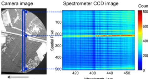
photo-Figure 4. Example scene from a flight along a highly reflecting mo-torway in the centre of the field of view. Left: visual image of the observed scene, the spectrometer field of view marked by the blue box. Right: intensity recording on the 2-D CCD chip, with spectral information distributed along the horizontal axis and spatial infor-mation on the vertical axis. The horizontal stripes on the CCD im-age are caused by the 35 light fibres, the enhanced intensity from the bright motorway being visible only in one of the fibres.
graph in black and white is shown; the simultaneous CCD image of the DOAS measurement is shown on the right. In the CCD image, the horizontal axis contains the spectral in-formation, while spatial information is distributed along the vertical axis. The blue box in the photograph marks the field of view for the DOAS observation. The CCD figure shows 35 illuminated stripes from the 35 glass fibres. The strongly reflecting motorway in the centre of the photograph causes high intensity only in one fibre, i.e. within one stripe on the CCD. Other features such as the smaller road above the mo-torway and the bright area towards the bottom of the pic-ture can also be distinguished in the CCD image. The good imaging quality also allows the fine mapping of the motor-way seen before in Fig. 3.
5.2 Spectral resolution and spectral response function
Due to image aberrations for off-axis object points, the SRF has a different shape and width for the different viewing an-gles. In addition, the image quality along the spatial axis is slightly degraded towards the detector edges. However, the individual spatial directions remain well separated. The nar-rowest SRF is that one of the central viewing direction with a FWHM (full width at half maximum) of 0.5 nm, while the outermost viewing directions have an SRF with a FWHM of around 1.0 nm. The experimental SRF measured at 435.8 nm with a HgCd calibration lamp is displayed in Fig. 5. From the centre to the outer directions, lighter colours are used. The viewing directions to the right are drawn as solid lines; directions to the left are drawn as dotted lines. With a sam-pling of 512 pix/41 nm=12.5 pix/nm, i.e. between 6 and 12 pix/FWHM, the Nyquist sampling theorem is well ful-filled. The broadening of the point spread function towards the outer directions is clearly visible. The central directions
Figure 5. Experimental slit functions of the AirMAP instrument for campaign conditions in June 2011. The spectral resolution lies between 0.5 and 1.0 nm for the central and the outer viewing direc-tions, respectively.
reveal good symmetry, while the two outermost viewing di-rections (VD 01 and 09) show some deviation in form of a dent to the right of the SRF centre. Most importantly, the SRF shape and width for each individual viewing direction are reasonably constant along the wavelength axis (not shown). Such a dependency may in general occur and would become more important for larger CCD chips. However, no variations in the SRF spectral shape were detected in laboratory tests with the AirMAP. This stability is required for accurate and consistent trace gas retrieval results.
6 Observations of NO2
The measurements of the AirMAP instrument have been used to retrieve trace gas absorption signals using the DOAS method. The current instrumental set-up allows observations within a spectral range of around 41 nm. For the present study, the recorded spectral range was from 412 to 453 nm. This spectral band covers strong spectral features of the NO2 absorption cross section.
6.1 Retrieval settings
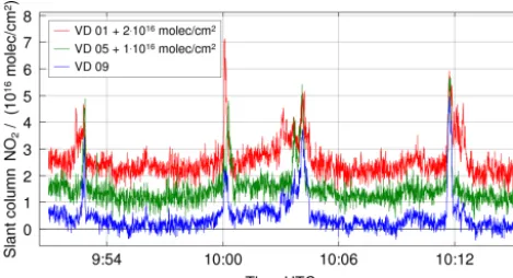
Figure 6. Excerpt of the NO2time series measured at high tem-poral resolution (0.5 s exposure time) during the flight on 4 June 2011, here for three of the nine viewing directions, VD 01, VD 05 and VD 09, offset against one another for better visibility. Signif-icant spatial variation of NO2 amounts is visible along the time axis (along track) as well as between the single viewing directions (across track).
product indicates that the stratospheric NO2 amount was about 4.0×10¹⁵molecules cm−2for the time and location of the research flight. The small diurnal variation of this strato-spheric NO2 column and the effect of changing the solar zenith angle (SZA) close to local noon are negligible. This is also because of the short time between the actual and the background measurement, which is 1 h at maximum for the measurements discussed in this study.
In addition to the NO2 absorption cross section (293 K, Burrows et al., 1998) the absorption signatures of O3(241 K, Burrows et al., 1999a), O4(296 K, Greenblatt et al., 1990) and H2O vapour (HITRAN 2004 data base, Rothman et al., 2005) are taken into account. A quadratic polynomial ac-counts for the broad-band spectral structures, and a constant intensity offset is fitted. In order to account for the in-filling of Fraunhofer lines in scattered light measurements, the Ring effect spectrum determined by radiative transfer calculations (Vountas et al., 2003) is also fitted as a pseudo-absorber. Prior to the actual retrieval procedure, all reference spectra are con-volved with the instrument’s SRF, individually for each view-ing direction.
6.2 NO2slant columns and retrieval quality
During the measurement flight, the retrieved SC of NO2 varies between values around 0 for areas which are similarly unpolluted as the rural reference region, and 5×10¹⁶molec cm−2for locations most strongly affected by local NOx emissions. Small negative SC values in some locations indicate cleaner conditions and thus lower NO2 amounts than in the reference region average. All results in this section refer to division of the field of view into nine viewing directions (referred to as LOS09 retrieval) at 0.5 s exposure time. A short part of the NO2slant column time se-ries is shown in Fig. 6, covering a 24 min period from 09:51
Figure 7. Example NO2fit results for 4 June 2011, 10:11:47 UTC, for three of the nine different viewing directions, VD 01, VD 05 and VD 09. The respective NO2slant columns are given in the figures.
to 10:15 UTC for three viewing directions, the furthest right (VD 01), centre (VD 05) and furthest left (VD 09) with re-spect to flight direction. Results of VD 01 and VD 05 are off-set against VD 09 for better visibility by 2×10¹⁶molec cm−2 and 1×10¹⁶molec cm−2, respectively. With an exposure time of 0.5 s this high-resolution time series shows signif-icant spatial variations along flight direction, i.e. along the time axis, as well as considerable spatial variation in across-flight direction, visible through the differences between the three viewing directions. Some of the variation is due to noise, which is in the range of a few times 1015molec cm−2 for the slant columns as discussed below. The observed vari-ations along and across flight direction are clearly larger than the noise alone.
Figure 8. Histograms for the distribution and variability of NO2 amounts in three of the nine different viewing directions used for uncertainty analysis. Data used for this figure are recorded 3 min around the 1 min reference (I0in the DOAS fit).
detection limit. Typical RMS values of the residual are in the range of (1.5–2.0)×10−3. As the spectral sampling is larger than necessary, the RMS may be improved by coadding along the spectral axis. However, such a procedure has no effect on the noise of the retrieved NO2amount.
The detection limits and uncertainties of the column re-sults are better estimated from the retrieved NO2 amounts and their noise. For this purpose, the spread of NO2values is analysed, taken from an area with small relative abundances (Platt and Stutz, 2008). In the present case, a suitable area is the reference location, from where the 1 min average ref-erence spectrumI0for the DOAS analysis is obtained. For better statistics, a 3 min section from the flight is used for the error analysis. Figure 8 shows the results for viewing di-rections VD 01, 05 and 09. The relative occurrence of the given NO2 column densities is plotted in a histogram with a bin width of 0.5×10¹⁵molec cm−2. The mean and the width of the distributions are found in each case by a fitted Gaussian function. The mean is slightly positive but close to 0 in all three cases (0.5–0.6×10¹⁵molec cm−2) due to residual background NO2. With 95 % probability, values lie within 2 times the standard deviation, 2σ, of 4.4, 3.5 and 5.5×10¹⁵molec cm−2 for VD 01, 05 and 09, respectively.
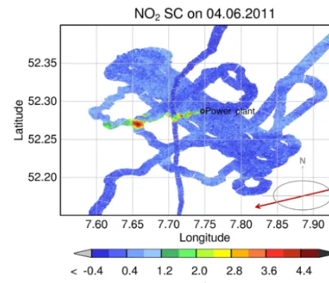
Figure 9. Map of NO2slant columns measured during the flight on 4 June 2011 above the area around the Ibbenbüren power plant. The elevated levels of NO2are clearly visible in the exhaust plume downwind of the power plant stack. In the bottom right corner of the map, the wind direction is indicated.
These values give a meaningful measure for the slant col-umn detection limit and uncertainty for individual detections. With typical air mass factors of around 2.2 (Sect. 6.3), the vertical column detection limit and uncertainty lie between 1.6 and 2.5×10¹⁵molec cm−2for a single observation, as-suming a normal distribution and using 2σto cover the range of possible values. As a result of some real variability in the NO2 amounts, these values represent an upper limit of the experimental uncertainty.
At a typical speed of 60 m s−1and 1100 m flight altitude, averaging over four subsequent measurements leads to nearly quadratic ground scenes with an area of 110×120 m, and the fit RMS is improved by nearly a factor of 2 as expected. In ar-eas affected by anthropogenic activities, NO2enhancements are clearly above the detection limit of the AirMAP instru-ment.
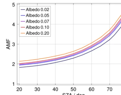
Figure 10. Box-air-mass-factors for NO2 calculated with SCIA-TRAN for flight geometries, 1.1 km flight altitude, 40◦SZA and different ground reflectance values.
viewing directions would have the tendency to always show larger values than others, neither in the instrument calibration parameters nor in the retrieved NO2column amount.
The location of the power plant is marked in the figure by a black dot. Enhanced amounts of NO2 are observed downwind of the power plant stack, while surrounding ar-eas have much lower NO2 amounts than within the ex-haust plume. The average wind direction is indicated in the map (see also Sect. 7.1). For single measurements, max-imum slant columns reach 5.0×10¹⁶molec cm−2. Typical amounts within the power plant plume are between 1.2 and 4×10¹⁶molec cm−2. This is much smaller than values mea-sured by Heue et al. (2008) above the huge South African Highveld power plants. In comparison, they observe slant columns up to 1.1×10¹⁷molec cm−2for the coal and syngas-fired Majuba power station (around 4100 MW nominal ca-pacity), and Melamed et al. (2003) observe vertical columns of up to 8×10¹⁶molec cm−2above the lignite-fired Monti-cello power station (Texas, USA, around 2000 MW nominal capacity).
6.3 Air mass factors for tropospheric NO2
In order to transfer the retrieved NO2slant columns into ver-tical column amounts, air mass factors (AMF) are computed by radiative transfer (RT) calculations. For this purpose, the SCIATRAN code is used (Rozanov et al., 2002). The AMF takes care of the relative light path length through the ab-sorber layer, and the vertical column (VC) is determined by
VC= SC
AMF(p). (6)
The AMF depends on a set of parameters p which deter-mine the radiative transfer scenario. This is influenced, e.g. by the wavelength, ground reflectance, the absorber profile, SZA and aerosols. The sensitivity of the measurements in dependence of the altitude location of the absorber is given
Figure 11. Air mass factors for NO2and their SZA dependence for different ground reflectance values for a NO2box profile of a mixed layer in the lowest 1 km.
by the Box-AMF, which is the respective AMF in a defined altitude range. For a scenario of 40◦SZA and a wavelength of 425 nm, the Box-AMF is plotted in Fig. 10 for different values of the ground reflectance and considering a flight al-titude of 1100 m and direct nadir LOS. SZA values for the campaign flight lie between 32 and 57◦, and for the cen-tral flight pattern, between 39 and 50◦. The flight took place on a clear summer day with good visibility; i.e. aerosols are not considered in these examples. The measurement sensi-tivity changes from 2.6 directly below the aircraft to values between 2.55 (20 % albedo) and 1.65 (5 % albedo) close to the ground. The sensitivity for NO2observation therefore de-pends on the trace gas altitude profile.
The path length of solar electromagnetic radiation through the layers below the aircraft also depends on the respective viewing angle, which for the AirMAP instrument reaches up to ±24◦ for level flight and even larger angles when the aircraft is banking and turning. The LOS influence on the AMF determined by RT calculations is only slightly differ-ent (<1 %) from the geometrically calculated factor. The AMF for nadir view (AMF0 for LOSα=0◦) is computed with SCIATRAN, and the correction for LOS angleθiis then based on the geometric AMFs,AMF[0andAMF[θi. With SZA
θs and LOSθi, the corrected VCθi for slant viewing
direc-tions is determined by
VCθi =SCθi·
1 AMFθi
≈SCθi·
1 AMF0
· AMF[0
[
AMFθi
(7)
with the geometric air mass factor
[
AMFθi= 1
cos(θs)
+ 1
cos(θi)
. (8)
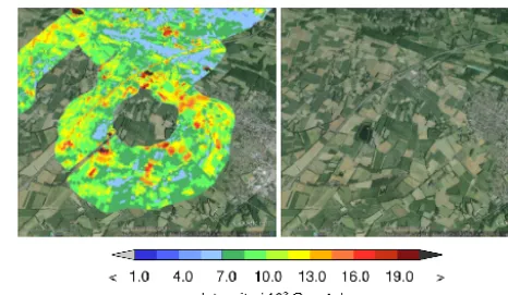
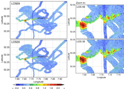
Figure 12. Map of NO2vertical columns above the Ibbenbüren power plant exhaust plume for division of the field of view into 9 LOS (top) and 35 LOS (bottom). On the right, a close-up view is shown. The retrieved slant columns from Fig. 9 and AMF from Fig. 11 (albedo 0.05, blue curve) have been used. Good consistency of NO2amounts is achieved independent of the LOS division.
5 %. In the vicinity of emission sources, the NO2will not be well mixed below the aircraft. Using Gaussian plume disper-sion, corresponding vertical profiles within an exhaust plume have been computed, and differences between plume pro-file AMFs and the Box-AMF have been investigated. The AMF for a plume at 6 km distance used below for emission estimates (Sect. 7) differs less than a few percent from the Box-AMF within the relevant SZA range, whereas for pro-files closer to the emitting stack, the plume is more confined and may cause a difference of about 5 % in the AMF.
It is worth noting that neither SCIATRAN nor the geo-metric approximation take 3-D effects into account. The im-portance of such 3-D effects increases for increasing SZA, increasing LOS angle and for a plume which is horizontally confined as well as situated at high altitudes directly below the aircraft. For such a case, an individual light beam may travel through the plume only once, e.g. either on the way from sun to the ground or from the ground to the instrument. In this case, the AMF would be overestimated and the result-ing vertical column would be underestimated. In addition, the assignment of the measured trace gas amount to the ground pixel may be affected. Multiple scattering, however, reduces the influence of 3-D effects.
Close to the stack, 3-D effects might be present in our case; further away from the stack, however, the plume has already spread in horizontal and vertical directions, so that the influ-ence of 3-D effects becomes less relevant.
6.4 NO2vertical columns
small as 0.4±8.5×10¹⁴molec cm−2within the central flight pattern.
The VC amounts of NO2 are strongly enhanced within a confined plume downwind of the power plant stack, as seen before. Maximum VC amounts reach up to 2.4×
1016molec cm−2, while typical values within the exhaust plume lie between 0.6 and 2.0×10¹⁶molec cm−2. NO2 amounts in overpasses closer to the stack are lower than in the overpasses further downwind, because emissions of ni-trogen oxides first occur as NO which is converted into NO2 during the transport in the plume. The most distant overpass at around 6 km reveals the largest NO2 amounts. In addi-tion, the plume broadens while it is transported away from the stack, and the integrated VC across the plume increases with distance from the stack. This is shown in more detail in the following section. In comparison to the NO2amounts within the plume, surrounding NO2values are rather small and variable below(4±2)×1015molec cm−2.
One flight segment in a north–south direction shows lower NO2amounts than the other flight paths. The respective seg-ment was flown latest in the pattern and at lower altitude; therefore the track is rather narrow. The later time means that the SZA and the influence of stratospheric NO2 have changed. This effect is noticeable but is too small to entirely explain the observed change in the background NO2. The lower flight altitude might cause some NO2to be missed by the measurements. Additional effects probably influence the measurements in this flight path, which is however not fur-ther used in this study.
Figure 12 demonstrates some further features of the imag-ing DOAS aircraft measurements. A comparably large area is covered with trace gas observations within a relatively short time interval at fine spatial resolution. The flight pattern above the target area with several partly overlapping flight legs was, e.g. completed within about 80 min. Hence, the ob-servations with AirMAP are useful for the analysis of small-scale trace gas variability above extended areas with several tens of kilometres’ side length.
7 Power plant emissions
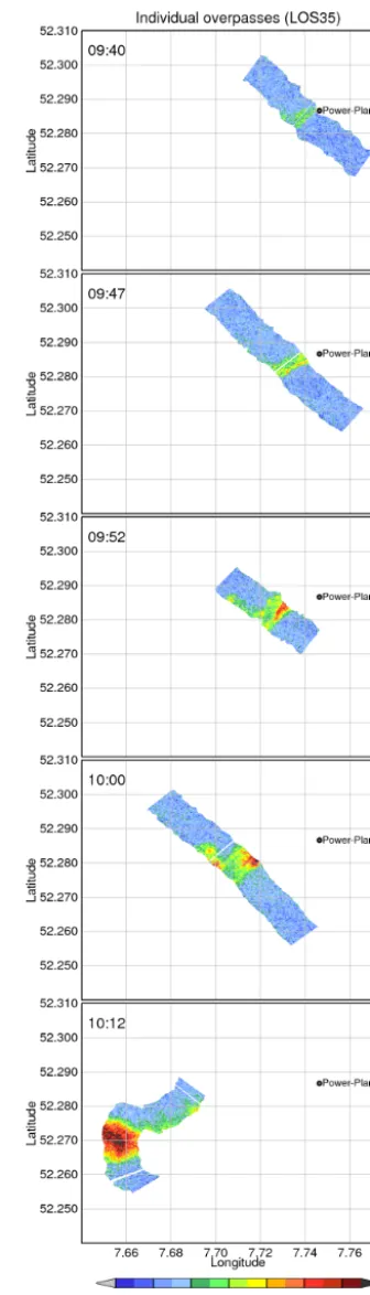
The NO2plume is investigated during several overpasses. In Fig. 13, five overpasses over the exhaust plume are displayed. They show the NO2 measurements at different distances downwind of the power plant stack. The overpass furthest away has a distance of around 6 km from the stack and is used for an emission estimate. Many details in the plume structure are resolved by the AirMAP measurements. At 09:40 UTC close to the stack, NO2 amounts are still rather low, as NO2 needs time to form from NO and ozone. Especially the two overpasses at 09:52 and 10:00 UTC show that the plume structure is strongly inhomogeneous. At 09:52 UTC the largest NO2amounts are not found in the lateral centre but towards the southern edge of the plume. At 10:00 UTC
Figure 14. Integrated NO2amount across the plume from five in-dividual overpasses (OP) at different times and distances from the stack. Results are taken from the LOS35 evaluation; therefore, in total, 175 cross sections through the plume are included in this dia-gram.
an interruption of the plume in wind direction (across track), i.e. a discontinuity due to atmospheric turbulence, is ob-served. Figure 14 shows the integrated NO2 amount across the plume with respect to the distance of the stack. The inte-grated NO2amount (line integral) takes into account the rel-ative angle between the cross section and the direction of the plume movement, i.e. the wind direction; see discussion be-low. Cross sections of the five overpasses are included in this figure, and data are based on the LOS35 evaluation. In total, the results from 175 cross sections are shown. The detailed maps of the plume and the integrated NO2amounts show that emission estimates from single cross sections would lead to fairly different results. NO2emission ratesQfrom the power plant point source are derived using the fifth cross section from the overpass furthest away from the stack. For this pur-pose, Gauss’s divergence theorem is utilized, describing the relation between the flux of a vector field through a closed surface (which is measured) to the divergence of the vector field inside the enclosed volume (which relates to the source strength). This relationship has also been used, e.g. by Wang et al. (2006), Heue et al. (2008) and Krings et al. (2013). Lo-cal wind data are a prerequisite for the emission Lo-calculations. 7.1 Wind data
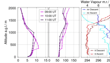
Information on wind speed and direction is received from the COSMO-DE regional model from the German Weather Ser-vice DWD (Doms and Baldauf, 2015). Observational data are assimilated, and the output grid size is 2.7×2.7 km2. The al-titude grid has 12 levels in the lowest kilometre. For the clos-est grid points around the target area, wind profiles (speed and direction) have been extracted. The wind speed on the campaign day was moderate, increases with altitude in the boundary layer and drops to smaller values above. Figure 15 shows the altitude profile of the wind speed (left) and direc-tion (middle) for a locadirec-tion close to the power plant (7.67◦E, 52.28◦N) for three hourly time steps at 09:00, 10:00 and
Figure 15. Example vertical profiles of wind speed (left) and wind direction (middle) from the COSMO-DE model on 4 June 2011 at three time steps (09:00, 10:00 and 11:00 UTC) for the location 7.67◦E, 52.28◦N, close to the Ibbenbüren power station, as well as potential temperature2, and water vapour mixing ratio m.r., during a dive south of the power plant (right).
Dl
VD 09 VD 01 Flight direction
(time, distance)
𝑢 𝑛 b
𝑢
VC (NO2)
i = 1 … n
Figure 16. Sketch illustrating the emission flux calculation from AirMAP data for an example plume overpass with wind vectoru, line element1l, flight path normal vectorn, angleβand NO2 ver-tical column VC(NO2). The contributionsito the emission source strengthQ(Eq. 11) are summed up along the transect.
Assuming Gaussian plume dispersion for the shape and development of the NO2 emission plume emerging at the stack altitude of 275 m a.g.l., the vertical plume extent can be estimated. Considering that the atmospheric stability class valid for the present campaign day was rated as slightly un-stable (Krings et al., 2013), dispersion leads to a substan-tial spreading of several hundred metres within the boundary layer at a distance of 6 km from the stack. From this percep-tion and the measurements of the vertical mixing layer ex-tent, a homogeneous distribution of NO2 below the aircraft is assumed for the wind averaging at this location. Below the aircraft, the wind speed varies between 6.1 and 9.2 m s−1 with an average of 8.3 m s−1. A small bias of+0.7 m s−1in the COSMO-DE wind speed data for the respective time and region has been identified by Krings et al. (2013) in com-parison to the AIMMS-20 wind probe. Taking the bias into account, a wind speed of 7.6 m s−1is used. The wind direc-tion varies between 61 and 75◦with an average of about 68◦. The AIMMS-20 wind probe on the aircraft yields a direction of 78◦ which is turned clockwise at the higher altitude of the aircraft position above the plume in agreement with the COSMO-DE profiles. The apparent plume transport from the measurements is consistent with a wind direction of around 70◦. For calculations, the 68◦angle is used, and uncertainties on this value are around±5◦.
7.2 Calculation and discussion of the emission rate
The aircraft measurements integrate over the vertical dimen-sion, so that the flux calculation considers the horizontal componentF=VC·uof the 3-D vector field of NO2 trans-port. VC is the NO2 vertical column and u is the effec-tive horizontal wind vector. The source strength (emission rate) Qis thus determined from the vertical NO2 columns measured within the exhaust plume. The divergence theorem yields
Q=
Z
A
∇FdA=
I
L
(F·ndl)=
I
L
VC·u·ndl. (9)
The integral runs over an areaAenclosed by the surrounding lineL. The calculated flux thus contains the emissions from all sources enclosed byL. For calculation ofQfrom the ex-perimental discrete data, the integral in Eq. (9) converts into a sum over the observed ground pixelsi:
Q =
I
L
VC·u·dl≈X
i
VCi·u·1li (10)
⇒Q = X
i
VCi·u·1licos(β). (11)
In the last step,βis the angle between the wind vectoruand the normal vector nof the line element along flight direc-tion 1l (or along any other selected transect). The product vanishes for pieces of the boundary Lwhich are parallel to
Figure 17. Cross section of NO2vertical columns through the ex-haust plume at around 10:12 UTC and a distance of around 6 km from the power plant used for the emission flux calculation. The cross section is taken from the ninth viewing direction of the LOS09 analysis.
the wind direction. Figure 16 illustrates the determination of
Qfrom the aircraft measurements with a simplified sketch of a plume overpass, including the parameters that enter the above calculation. When closing the integral over the sur-rounding line around the power plant on the upwind side of the power plant, positive NO2 amounts lead to a reduction of the resulting emission rate as the wind and line normal vectors are antiparallel.
The cross section through the plume along flight di-rection for one example viewing didi-rection (VD 09 from the LOS09 retrieval) is seen in Fig. 17. The cross sec-tion shows enhanced NO2 amounts at around 10:12 UTC up to 1.9×10¹⁶molec cm−2, clearly above the background amount in a compact shape. Immediately to the sides of the central plume, a mean vertical NO2 column of VCB= 2×10¹⁵molec cm−2is observed, resulting from background NO2concentrations and outflow from the city of Ibbenbüren. Parts of the city of Ibbenbüren are close to the power plant and are therefore enclosed by any possible flight path. The additional sources can influence the emission estimate if the closed line integral is determined. Alternatively, the back-ground NO2is assumed constant across the plume and sub-tracted from the observed NO2 in order to effectively re-move additional emission sources. The emission rate is then determined by the downwind part of the line integral over the background corrected NO2 column VC−VCB. Calcu-lated this way, the emission rate is slightly smaller than from the closed integral; however, the differences are not signif-icant. Other local sources can therefore be concluded to be small. Figure 18 shows the computed emission rates with re-spect to the distance from the power plant location for the nine viewing directions, i.e. nine independent results forQ. From this, the average emission rate and standard deviation is
¯
Figure 18. Emission flux estimates from the plume overpass at around 6 km distance for the nine different viewing directions.
of the mean when considering the uncertainties on the indi-vidual results ofQ. The uncertainties on all involved quanti-ties making up for the error bars in Fig. 18 are discussed in Sect. 8 below.
7.3 Comparison to emission reports
The determined emission rates correspond to 82±20 g s−1 NO2. For the conversion into a NOx emission rate, a value for the [NO]/[NO2] ratiorneeds to be assumed. The ratio
r is the inverse of the well-known “Leighton ratio”, which is the ratio [NO2]/[NO] in photo-stationary state. The NOx emission rateQNOx is then given by
QNOx=(1+r)·QNO2. (12)
A value ofr=0.25 is used (Ehhalt et al., 1992), which is rea-sonable as soon as steady state is achieved; see discussions below. Following from this, the NOx emission rateQNOx is
103±25 g s−1NOx in mass of NO2. The error does not in-clude uncertainties of the ratio r. Reports issued in the E-PRTR state an emission rate of 3060 t a−1 NO
x in mass of NO2. Extrapolating the instantaneous observations from the individual overflight to an entire year, the observed annual emission rate would be 3240±800 t a−1, consistent with the reported amounts. The extrapolation is only reasonable either if the emission rate is constant over the course of the year, or if the individual day was a representative situation of typical conditions, which is both not necessarily the case. However, the comparison shows that the plume estimate of NOx emis-sions and the reported annual average are consistent. 7.4 Limitations of the emission calculations
At example locations closer to the stack, the analysis leads to lower NOxemission rates. The reason for this is that less of the emitted NO has been converted to the measured NO2
(Davis et al., 1974). For application of the divergence the-orem, chemical inertness of the compound or a stationary state condition needs to be assumed. However, NO2 is not inert at atmospheric conditions. For a meaningful reasoning, the distance of the NO2measurement from the power plant needs to be sufficiently large so that the photochemical sta-tionary state can be assumed as implied above. Stasta-tionary state will evolve over the first few tens of kilometres of an ex-haust plume (Davis et al., 1974). The actual distance required depends on wind speed and atmospheric stability as well as chemical conversions mainly driven by reactions with O3and photolysis. Wind speed is moderate, and at around 6 km dis-tance, an air parcel has travelled for nearly 15 min from the stack. At large NO concentrations, O3 can be entirely de-pleted in the plume centre. NOx emissions are smaller in the present case as compared to Davis et al. (1974). If O3 is not entirely depleted, conversion to NO2and achievement of a steady state evolves faster. If a steady state has not been reached, the factorr and hence alsoQNOx would be larger
than estimated above. In conclusion, estimates of the NOx emission rate are derived here under these limitations. 7.5 Non-uniform plume dispersion
The NO2amounts within the emission plume do not show a smooth and uniform distribution. The emission rates plotted in Fig. 18 represent nine independent results forQat differ-ent distances from the stack, i.e. differdiffer-ent times since emis-sion. The approximate time difference between two adjacent viewing directions, taking the locations and wind speed into account, is about 13 s; the difference between the outermost directions is about 2 min. Even from this short excerpt of the emission plume, its variability becomes clear. Possibly the NO emissions in the first place, but mainly the chemical conversions and the transport process are presumably non-uniform. The particularly inhomogeneous structure of the plume was addressed in Figs. 13 and 14, where overpasses closer to the stack are included as well. In this respect, obser-vations made with the AirMAP instrument provide a good opportunity to study these plume processes within short time and spatial scales and covering distances of many kilometres.
8 Error estimates
of the reference location for the reference spectrum I0 in the DOAS retrieval does not affect the emission calculation, and hence also not its uncertainty. From all considered er-ror sources, an overall relative and additional absolute un-certainty of around ±30 % and ±2.5×10²³molec s−1, re-spectively, is determined for the instantaneous emission rate
QNO2.
8.1 Uncertainties of the vertical NO2columns
The NO2 DOAS retrieval exhibits fitting errors around 5 % for large NO2 values within the plume. Naturally, the rel-ative error becomes bigger for small NO2 abundances to the sides of the plume. Absolute errors lie in the range of 2×10¹⁵molec cm−2. The same absolute uncertainty applies for the background NO2 amount, determined next to the emission plume. Systematic errors induced by the choice of NO2cross section are in the range of a few percent, e.g. the temperature dependence causes an uncertainty of<2 % for a temperature change from surface to 2 km of about 15 K (from 297 to 282 K, based on COSMO-DE data), when using a 293 K reference cross section.
Main uncertainties of the NO2VC arise from assumptions necessary for the calculation of the AMF, e.g. through influ-ences from aerosol scattering, the vertical NO2 profile and ground albedo. While aerosol above a remotely sensed NO2 layer tends to shield part of the trace gas, mixed aerosol with NO2 may also lead to enhanced sensitivity, e.g. shown for satellite-specific studies (Leitão et al., 2010). The campaign day was a fairly clear and sunny day with good visibility. Therefore, the error from assuming there to be no aerosol scattering in the radiative transfer is not large. Conversely to the NO2 vertical profile, which in general is not known, the emission plume injection height and the height of the mixed layer are approximately known. AMFs for different profiles, box-shaped and Gaussian plumes, as well as for dif-ferent ground albedo values, have been computed (Sect. 6.3). From the related uncertainties, deviations of the AMF in the range of 25 % are considered.
8.2 Uncertainties of the path element length
Factors influencing the calculation of the length of the path element in the line integral include the timing of the GPS sig-nal, the uncertainties in the GPS positioning itself and in the aircraft orientation and altitude. In comparison to the preci-sion and accuracy of the GPS position and its timing, which lead to an uncertainty of a few metres only, the influence of the aircraft angles are the dominant ones. Also, the inac-curacy of the altitude is small in comparison. Uncertainties in the pitch and roll angles, of around 0.5–1◦ each, cause displacements on the ground, leading to an overall error of around 30 m for the geolocation in our case, i.e. when fly-ing at the main altitude of around 1100 m. However, it is the difference in geolocation between the start and end of the
measurements that is entered in the emission calculation in Eq. (11), which causes a major part of the systematic uncer-tainty of the angles to be cancelled out. A curvature in the flight path during overpass (cf. Fig. 13) induces an inaccu-racy as the path is approximated by straight segments leading to a systematic but small underestimation of the track length. Overall, the influence of the path length uncertainty is minor in comparison to the other error sources.
8.3 Uncertainties of the wind speed and direction The wind speed and direction imply errors (a) due to uncer-tainties and inaccuracies in the model data itself, (b) due to the finite grid size and (c) due to uncertainties in the vertical expansion of the emission plume. Depending on the time of day and the lifting of the boundary layer, the variation of the wind speed and direction with altitude can be fairly strong. From estimates of the plume vertical location and extension, related uncertainties on the order of 10 % for the wind speed and 5 % on the cosine of relative wind angleβ are reason-able. The latter is true as long asβ <30◦, which is the case for the analysed overpass.
9 NO2above motorways
As the AirMAP instrument offers high spatial resolution and good quality NO2 measurements, it is worth investigating weaker and smaller NO2 sources. The flight path also fol-lowed motorways in north-west Germany. Figure 19 shows a flight section along the A1 motorway for about 5 min around 08:50 UTC. The recorded intensity is shown in the left map, where the motorway can clearly be distinguished by higher intensity values in comparison to surrounding vegetation, again demonstrating the good imaging capability of AirMAP. Some bright reflecting fields in the western part of the track yield even higher intensities than the road surface. The two maps on the right cover an excerpt of the section for the re-flected intensity (top right) and the retrieved NO2amounts (bottom right), all from the LOS35 retrieval. With a flight altitude of 1500 m and an airspeed of 90 m s−1, the individ-ual ground pixel is 40×45 m2in across×along track size. Enhanced NO2values of around 5×10¹⁵molec cm−2are de-tected above the motorway. The AMF causes signal enhance-ment of the NO2amounts above the bright surface due to an increased albedo and will need to be considered for more pre-cise calculations. However, while the intensity (Int) is larger above the bright field than above the motorway, NO2is only enhanced above the road. The following values are deduced from 23 observations (ground pixels) above the motorway and 30 observations above the bright field:
– for the motorway: VC=5±2×10¹⁵molec cm−2 and Int=(14±2)×103counts s−1;
The enhanced reflectivity from the road surface is therefore not sufficient to explain the retrieved NO2amounts. In con-clusion, enhanced NO2 from motor vehicle emissions from the motorway is clearly observed.
In previous studies, Pundt et al. (2005) used a tomographic DOAS approach to measure NO2 emissions from a Ger-man motorway, the A656, at a fixed ground location. This study was used in order to compare the order of magnitude of NO2column amounts for a medium-sized highway. They found enhancement of NO2on the order of 5–10 ppb above the background level in the lowest few tens of metres, with measurement data being collected between the surface and 40 m altitude. By vertically integrating these numbers, the column amount is around 0.4–0.8×10¹⁵molec cm−2above background. NO2 amounts decrease with altitude, but any NO2 present at higher altitudes originating from the traffic emissions is not included. Following the Federal Highway Research Institute (Bundesanstalt für Straßenwesen, BASt), the vehicle number frequencies for the respective motorway sections of the A656 and A1, respectively, are both in the same range of around 55 000 vehicles on average in 24 h when considering both travel directions (http://www.bast.de, last visited 19 December 2013). The above observations from aircraft yield a column of 3.0±2.2×10¹⁵molec cm−2NO2 above background for the A1, which is larger than that from the tomographic experiment over the A656, but lies in a com-parable and reasonable range. The difference is a result of the typically strong variations in time of the instantaneous traffic densities and flow, and is also influenced by the vertical con-finement of the A656 data used here from Pundt et al. (2005). It is relevant to add that an overestimation of the NO2 verti-cal column from the AirMAP data as a result of the road surface reflectivity is not large, and cannot account for the difference between the two motorway NO2values. Assum-ing an albedo of 0.2 instead of 0.05, even in a clear Rayleigh atmosphere, the overestimation is below 23 % for NO2at the surface, where the albedo influence is largest (cf. Fig. 10). For elevated layers or in the presence of aerosols, this effect is even smaller.
The ability of AirMAP to map pollutants emitted from transport is especially advantageous when aiming to im-prove emission inventories and the predictive capability of regional modelling. Regular aircraft measurement campaigns focussing on motor traffic emissions that are complementary and coupled to the network of ground-based stations may provide invaluable insight into these variable pollutant emis-sions and distributions.
10 Conclusions and outlook
The AirMAP imaging DOAS instrument has been charac-terized and was successfully applied during an airborne op-eration in June 2011. In its current set-up, the instrument is adjusted for measurements of NO2column amounts
be-low the aircraft. The AirMAP instrument and associated data analysis differ from previous studies in several aspects. The present study demonstrates the mapping of compara-bly small-scale NO2 abundances at good spatial coverage and resolution. The wide and continuous spatial coverage is achieved by (a) a wide field of view of 48◦across track and (b) a measurement sequence without temporal gaps between consecutive exposures. Independent of flight altitude, the in-strument provides smooth trace gas maps. The inin-strument is hence capable of covering large areas with trace gas obser-vations within a comparably short time. Previously reported instruments with opening angles up to 30◦ require nearly twice the length of time to cover the same area. As an exam-ple, AirMAP would achieve full coverage of a typical satel-lite pixel of GOME-2 (40×80 km2) or OMI (13×24 km2) at a flight altitude of around 3 km, and an air speed around 80 m s−1, within 4.5 h or less than 1 h, respectively, with pixel sizes below 100 m side length at full resolution of 35 viewing directions.
Flexible integration of the instrument into the aircraft is facilitated through an optical light guide with sorted fibres, allowing up to 35 individual viewing directions simulta-neously. At full spatial resolution, a ground pixel size of 30×30 m2is enabled for present flight conditions. At such fine spatial resolution, accurate geolocation of the observa-tions is required. In contrast to some previous studies on air-borne NO2measurements, the aircraft attitude is taken fully into account. In relation to the pixel sizes, computed dis-placements are significant for the investigated survey flight. Accurate geolocation has been achieved during typically un-level flight conditions and even during strongly curved flight paths by use of AHRS positioning data. Good spatial imag-ing and the accurate assignment of the observations to ground locations have been demonstrated.
Figure 19. Flight section along the motorway A1 in north-west Germany. The recorded intensity (left) is enhanced above the motorway and in addition above bright fields. The two maps on the right show an excerpt of the flight section, the recorded intensity (top) and the NO2 VC (bottom). The reflected intensity is enhanced above the motorway and even more above a field on the western side of the swath. NO2 amounts above the motorway are also enhanced, but not above the bright field.
and analysis of exhaust plumes and their temporal evolution, also in future applications. At full spatial resolution, local enhancements of NO2columns above a motorway have been detected and investigated for a short flight section as an illus-tration of the potential of the AirMAP small-scale observa-tions. Such observations in a campaign or on a regular ba-sis are invaluable for the improvement of emission inven-tories and as a reference for regional modelling. The cur-rent spectrometer configuration was focussed on NO2; mi-nor modifications in the spectrometer set-up enable observa-tions of other key trace gases such as formaldehyde, HCHO, and glyoxal, CHOCHO, as well as sulfur dioxide, SO2, water vapour, H2O, and halogen oxides (BrO, OClO and IO).
In conclusion, the present study demonstrates the success-ful operation of the AirMAP instrument, in particular the achievement of good spatial resolution and coverage, as well as the high instrument quality in terms of spatial imaging and accurate geolocation. Good spectral quality and stability support the successful observation of NO2on small spatial scales. The good mapping capability of AirMap is to be used in the future for scientific investigations focussing on small-scale spatial variability of tropospheric trace species.
Acknowledgements. Financial support for the AirMAP project by the State and University of Bremen is gratefully acknowledged. The project is supported through the University of Bremen Insti-tutional Strategy in the framework of the Excellence Initiative. The AIRMETH-2011 campaign was jointly funded by the Alfred
We-gener Institute for Polar and Marine Sciences (AWI), the Helmholtz Centre Potsdam (German Research Centre for Geosciences, GFZ) and the University of Bremen.
The authors are grateful to AWI Bremerhaven and Fielax, especially to Martin Gehrmann and Franziska Nehring, for their dedicated and essential campaign support. Support by the AIRMETH team is acknowledged for including AirMAP in the campaign configuration. The Polar-5 aircraft was kindly operated by Kenn Borek Air Ltd, Canada. COSMO-DE model data were obtained from the German Weather Service (DWD). The authors are thankful to Thomas Krings for discussions on the wind data, and to Vladimir Rozanov for his support on the RT code SCIATRAN.
The article processing charges for this open-access publication were covered by the University of Bremen.
Edited by: J. Stutz
References
Baidar, S., Oetjen, H., Coburn, S., Dix, B., Ortega, I., Sinreich, R., and Volkamer, R.: The CU Airborne MAX-DOAS instrument: vertical profiling of aerosol extinction and trace gases, Atmos. Meas. Tech., 6, 719–739, doi:10.5194/amt-6-719-2013, 2013. Beirle, S., Platt, U., Wenig, M., and Wagner, T.: Weekly cycle of
Berg, N., Mellqvist, J., Jalkanen, J.-P., and Balzani, J.: Ship emis-sions of SO2and NO2: DOAS measurements from airborne plat-forms, Atmos. Meas. Tech., 5, 1085–1098, doi:10.5194/amt-5-1085-2012, 2012.
Bobrowski, N., Hönninger, G., Lohberger, F., and Platt, U.: IDOAS: A new monitoring technique to study the 2D distribution of vol-canic gas emissions, J. Volcanol. Geotherm. Res., 150, 329–338, doi:10.1016/j.jvolgeores.2005.05.004, 2006.
Brewer, A. W., McElroy, C. T., and Kerr, J. B.: Nitrogen dioxide concentrations in the atmosphere, Nature, 246, 129–133, 1973. Bruns, M.: NO2 Profile Retrieval using Airborne Multiaxis
Dif-ferential Optical Absorption Spectrometer (AMAXDOAS) data, Ph.D. thesis, University Bremen, 2004.
Bruns, M., Buehler, S. A., Burrows, J. P., Heue, K.-P., Platt, U., Pundt, I., Richter, A., Rozanov, A., Wagner, T., and Wang, P.: Retrieval of Profile Information from Airborne Multi Axis UV/visible Skylight Absorption Measurements, Appl. Optics, 43, 4415–4426, 2004.
Bruns, M., Buehler, S. A., Burrows, J. P., Richter, A., Rozanov, A., Wang, P., Heue, K. P., Platt, U., Pundt, I., and Wagner, T.: NO2 Profile retrieval using airborne multi axis UV-visible skylight absorption measurements over central Europe, Atmos. Chem. Phys., 6, 3049–3058, doi:10.5194/acp-6-3049-2006, 2006. Bucsela, E., Celarier, E., Wenig, M., Gleason, J., Veefkind, J.,
Boersma, K., and Brinksma, E.: Algorithm for NO2vertical col-umn retrieval from the ozone monitoring instrument, Geoscience and Remote Sensing, IEEE Transactions on, 44, 1245–1258, doi:10.1109/TGRS.2005.863715, 2006.
Burrows, J. P., Dehn, A., Deters, B., Himmelmann, S., Richter, A., Voigt, S., and Orphal, J.: Atmospheric remote sensing ref-erence data from GOME: Part 1. temperature dependent absorp-tion cross-secabsorp-tions of NO2in the 231-794 nm Range, J. Quant. Spectrosc. Ra. Transfer, 60, 1025–1031, 1998.
Burrows, J. P., Richter, A., Dehn, A., Deters, B., Himmelmann, S., Voigt, S., and Orphal, J.: Atmospheric remote-sensing refer-ence data from GOME: Part 2. Temperature-dependent absorp-tion cross secabsorp-tions of O3 in the 231-794 nm range, J. Quant. Spectrosc. Ra. Transfer, 61, 509–517, doi:10.1016/S0022-4073(98)00037-5, 1999a.
Burrows, J. P., Weber, M., Buchwitz, M., Rozanov, V. V., Ladstätter-Weissenmayer, A., Richter, A., DeBeek, R., Hoogen, R., Bram-stedt, K., and Eichmann, K. U.: The Global Ozone Monitoring Experiment (GOME): Mission Concept and First Scientific Re-sults, J. Atmos. Sci., 56, 151–175, 1999b.
Davis, D. D., Smith, G., and Klauber, G.: Trace Gas Analysis of Power Plant Plumes Via Aircraft Measurement: O3, NO, and SO2Chemistry, Science, 186, 733–736, 1974.
Dix, B., Brenninkmeijer, C. A. M., Frieß, U., Wagner, T., and Platt, U.: Airborne multi-axis DOAS measurements of atmospheric trace gases on CARIBIC long-distance flights, Atmos. Meas. Tech., 2, 639–652, doi:10.5194/amt-2-639-2009, 2009. Doms, G. and Baldauf, M: A Description of the Nonhydrostatic
gional COSMO-Model, Deutscher Wetterdienst, Technical Re-port, May 2015, available at: http://www.cosmo-model.org/, last access: December 2015.
Ehhalt, D. H., Rohrer, F., and Wahner, A.: Sources and Distribution of NOxin the Upper Troposphere at Northern Mid-Latitudes, J. Geophys. Res., 97, 3723–3738, 1992.
Galloway, J., Likens, G., Keene, W., and Miller, J.: The Composition of precipitation in the remote areas of the world, J. Geophys. Res.-Oceans and Atmos., 87, 8771–8786, doi:10.1029/JC087iC11p08771, 1982.
General, S., Pöhler, D., Sihler, H., Bobrowski, N., Frieß, U., Ziel-cke, J., Horbanski, M., Shepson, P. B., Stirm, B. H., Simpson, W. R., Weber, K., Fischer, C., and Platt, U.: The Heidelberg Airborne Imaging DOAS Instrument (HAIDI) – a novel imag-ing DOAS device for 2-D and 3-D imagimag-ing of trace gases and aerosols, Atmos. Meas. Tech., 7, 3459–3485, doi:10.5194/amt-7-3459-2014, 2014.
General, S., Bobrowski, N., Pöhler, D., Weber, K., Fischer, C., and Platt, U.: Airborne I-DOAS measurements at Mt. Etna: BrO and OClO evolution in the plume, J. Volcanol. Geotherm. Res., 300, 175–186, 2015.
Gerilowski, K., Tretner, A., Krings, T., Buchwitz, M., Bertagnolio, P. P., Belemezov, F., Erzinger, J., Burrows, J. P., and Bovens-mann, H.: MAMAP – a new spectrometer system for column-averaged methane and carbon dioxide observations from aircraft: instrument description and performance analysis, Atmos. Meas. Tech., 4, 215–243, doi:10.5194/amt-4-215-2011, 2011. Greenblatt, G. D., Orlando, J. J., Burkholder, J. B., and
Ravis-hankara, A. R.: Absorption Measurements of Oxygen Between 330 and 1140 nm, J. Geophys. Res., 95, 18577–18582, 1990. Heue, K.-P., Richter, A., Bruns, M., Burrows, J. P., v. Friedeburg, C.,
Platt, U., Pundt, I., Wang, P., and Wagner, T.: Validation of SCIA-MACHY tropospheric NO2-columns with AMAXDOAS mea-surements, Atmos. Chem. Phys., 5, 1039–1051, doi:10.5194/acp-5-1039-2005, 2005.
Heue, K.-P., Wagner, T., Broccardo, S. P., Walter, D., Piketh, S. J., Ross, K. E., Beirle, S., and Platt, U.: Direct observation of two dimensional trace gas distributions with an airborne Imag-ing DOAS instrument, Atmos. Chem. Phys., 8, 6707–6717, doi:10.5194/acp-8-6707-2008, 2008.
Heue, K.-P., Brenninkmeijer, C. A. M., Baker, A. K., Rauthe-Schöch, A., Walter, D., Wagner, T., Hörmann, C., Sihler, H., Dix, B., Frieß, U., Platt, U., Martinsson, B. G., van Velthoven, P. F. J., Zahn, A., and Ebinghaus, R.: SO2 and BrO observa-tion in the plume of the Eyjafjallajökull volcano 2010: CARIBIC and GOME-2 retrievals, Atmos. Chem. Phys., 11, 2973–2989, doi:10.5194/acp-11-2973-2011, 2011.
Hilboll, A., Richter, A., and Burrows, J. P.: Long-term changes of tropospheric NO2 over megacities derived from multiple satellite instruments, Atmos. Chem. Phys., 13, 4145–4169, doi:10.5194/acp-13-4145-2013, 2013.
Hönninger, G., von Friedeburg, C., and Platt, U.: Multi axis dif-ferential optical absorption spectroscopy (MAX-DOAS), Atmos. Chem. Phys., 4, 231–254, doi:10.5194/acp-4-231-2004, 2004. Ibrahim, O., Shaiganfar, R., Sinreich, R., Stein, T., Platt, U., and
Wagner, T.: Car MAX-DOAS measurements around entire cities: quantification of NOx emissions from the cities of Mannheim and Ludwigshafen (Germany), Atmos. Meas. Tech., 3, 709–721, doi:10.5194/amt-3-709-2010, 2010.