www.atmos-meas-tech.net/6/3257/2013/ doi:10.5194/amt-6-3257-2013
© Author(s) 2013. CC Attribution 3.0 License.
Atmospheric
Measurement
Techniques
Improvements to the OMI near-UV aerosol algorithm using A-train
CALIOP and AIRS observations
O. Torres1, C. Ahn2, and Z. Chen2
1NASA Goddard Space Flight Center, Greenbelt, Maryland, 20771, USA 2Science Systems and Applications, Inc., Lanham, Maryland, 20706, USA
Correspondence to: O. Torres ([email protected])
Received: 19 April 2013 – Published in Atmos. Meas. Tech. Discuss.: 21 June 2013 Revised: 7 October 2013 – Accepted: 14 October 2013 – Published: 27 November 2013
Abstract. The height of desert dust and carbonaceous
aerosols layers and, to a lesser extent, the difficulty in deter-mining the predominant size mode of these absorbing aerosol types, are sources of uncertainty in the retrieval of aerosol properties from near-UV satellite observations. The avail-ability of independent, near-simultaneous measurements of aerosol layer height, and aerosol-type related parameters de-rived from observations by other A-train sensors, makes possible the use of this information as input to the OMI (ozone monitoring instrument) near-UV aerosol retrieval al-gorithm (OMAERUV). A monthly climatology of aerosol layer height derived from observations by the CALIOP (Cloud-Aerosol Lidar with Orthogonal Polarization) sensor, and real-time AIRS (Atmospheric Infrared Sounder) carbon monoxide (CO) observations are used in an upgraded version of the OMAERUV algorithm. AIRS CO measurements are used as an adequate tracer of carbonaceous aerosols, which allows the identification of smoke layers in regions and sea-sons when the dust-smoke differentiation is difficult in the near-UV. The use of CO measurements also enables the iden-tification of high levels of boundary layer pollution unde-tectable by near-UV observations alone. In this paper we dis-cuss the combined use of OMI, CALIOP and AIRS observa-tions for the characterization of aerosol properties, and show an improvement in OMI aerosol retrieval capabilities.
1 Introduction
Since the discovery of the near-UV capability of absorb-ing aerosols detection from space over a decade ago (Hsu et al., 1996; Herman et al., 1997; Torres et al., 1998), the
UV Aerosol Index (AI), calculated from observations by the Total Ozone Mapping Spectrometer (TOMS) family of sen-sors, and more recently by the Ozone Monitoring Instrument (OMI), has been used to map the daily global distribution of UV-absorbing aerosols such as desert dust particles as well as carbonaceous aerosols generated by anthropogenic biomass burning and wildfires (Herman et al., 1997), and volcanic ash injected in the atmosphere by volcanic eruptions (Seftor et al., 1999). The AI concept for aerosol detection has also been applied to other near-UV capable sensors such as GOME (Gleason et al., 1998; De Graaf et al., 2005a), and SCIA-MACHY (de Vries et al., 2009; De Graaf et al., 2005b).
In addition to the qualitative AI product, near-UV retrieval algorithms of aerosol extinction optical depth (AOD) and single scattering albedo (SSA) making use satellite mea-surement in the 330–388 nm range have been applied to the TOMS (Torres et al., 1998, 2002) and OMI (Torres et al., 2007; Ahn et al., 2008) observations. The quantitative inter-pretation of the near-UV measurements in terms of aerosol absorption, however, is affected by the dependency of the measured radiances on the height of the absorbing aerosol layer (Torres et al., 1998; De Graaf et al., 2005a), and the difficulty in differentiating between carbonaceous and desert dust aerosol types, especially over land.
The near-simultaneity of satellite observations by a plural-ity of A-train sensors, provides the unprecedented opportu-nity of combining time- and space-collocated radiance ob-servations and/or derived atmospheric parameters for global climate analysis (Anderson et al., 2005). Combined A-train observations can also be used in inversion algorithms to fur-ther constrain retrieval conditions and, thus, reduce the need for assumptions. CALIOP (Cloud-Aerosol Lidar with Or-thogonal Polarization) measurements of the vertical distri-bution of the atmospheric aerosol load, and Atmospheric In-frared Sounder (AIRS) carbon monoxide (a suitable tracer of carbonaceous aerosols) observations, provide information that can be used to prescribe aerosol layer height and de-termine aerosol type in the OMI near-UV aerosol algorithm (OMAERUV).
In this paper we discuss the use of observations by A-train sensors CALIOP and AIRS, on aerosol layer height and CO to provide reliable information on aerosol layer height and aerosol type as input to OMAERUV. In Sect. 2, we briefly describe an improved version of the OMAERUV algorithm that utilizes CALIOP and AIRS observations as ancillary in-formation. A detailed description of the way AIRS CO data is used in the OMI aerosol inversion procedure is presented in Sect. 3, followed by a discussion of the development of a CALIOP-based aerosol layer height climatology in Sect. 4, and an evaluation of the improved accuracy of OMI retrievals using AERONET observations in Sect. 5. Summary and final remarks are presented in Sect. 6.
2 The OMAERUV algorithm
OMI is a spectrograph that measures upwelling radiances at the top of the atmosphere in the range 270–500 nm (Levelt et al., 2006) since its deployment in 2004. With a 2600 km across-track swath, and sixty viewing positions, it provided nearly daily global coverage at a 13×24 km nadir resolu-tion (28×150 at extreme off-nadir) during the first three years of operation. Since mid-2007, an external obstruction to the sensor’s field of view, perturbing OMI measurements of both solar flux and Earth shine radiance at all wave-lengths, began to progressively develop. Currently, about half the sensor’s sixty viewing positions are affected by what is referred to as “row anomaly”, since the viewing posi-tions are associated with the row numbers on the CCD de-tectors. The site http://www.knmi.nl/omi/research/product/ rowanomaly-background.php provides details on the onset and progression of the row anomaly.
The OMAERUV algorithm uses as input measured re-flectances at 354 and 388 nm to retrieve column atmosphere values of AOD and single SSA. Ancillary information on near-UV (354 and 388 nm) surface albedo (Aλ), scene type,
and aerosol layer height (ALH) is required. Values of sur-face albedo are obtained from a TOMS-based long-term cli-matology of minimum reflectivity similar to that of Herman
and Celarier (1997), modified to account for the darkening effect of strongly absorbing aerosols. Real-time AIRS CO measurements are used to identify carbonaceous particles, and ALH is inferred based on CALIOP measurements. The ways AIRS CO and CALIOP aerosol height information are used in the OMAERUV algorithm is the central theme of this paper, and it is discussed at length in Sects. 3 and 4.
2.1 Aerosol models and forward calculations
The algorithm assumes that the atmospheric aerosol column can be represented by one of three aerosol types: desert dust (DD), carbonaceous particles (CB), and sulfate-based (SF) aerosols. Each aerosol type is characterized by a fixed bi-modal spherical particle size distribution (Torres et al., 2007) with parameters derived from long-term AERONET statis-tics (Dubovik et al., 2002). The relative spectral dependence of the imaginary component of refractive in the 354–388 nm range,1k, is assumed for each aerosol type (Torres et al., 2007), and has been recently modified for the CB type to ac-count for the absorption effects of organic carbon (Jethva and Torres, 2011). Each aerosol type is further divided into seven sub-types to account for the variability of the imaginary com-ponent of the refractive index at 388 nm,k388, which, in
com-bination with the assumed size distribution, translates into SSA variability.
Forward radiative transfer calculations of upwelling re-flectance at the top of the atmosphere (354 and 388 nm) for the resulting 21 aerosol models were used to generate a set of look-up tables (LUTs) with nodal points in viewing geome-try, AOD, SSA, ALH.
2.2 Inversion procedure
The measured reflectances are first used to calculate the scene 388 nm Lambert Equivalent Reflectivity (R388), and
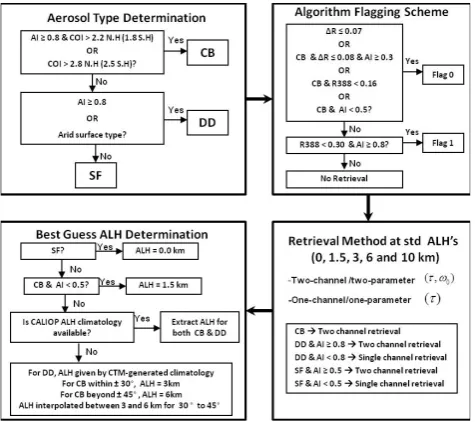
Fig. 1. Graphic description of OMAERUV inversion scheme.
The absorbing aerosol type identification is achieved by examining the values of AI and COI in relation to threshold values AI0 and COI0 that represent, respectively, AI noise
and background COI values not necessarily associated with the free troposphere CO burden which is expected to co-exist with the lofted carbonaceous aerosols (Andreae and Metlet, 2001). Adopted threshold values of COI0correspond to the
average of AIRS CO climatological annual minima over ma-jor biomass-burning/boreal fire activity regions. Such values are 2.2 in the Northern Hemisphere and 1.8 for the South-ern Hemisphere, based on Yurganov et al. (2008, 2010). The value of AI0 (0.8 for both land and ocean conditions), is a
slightly smaller value that the one used in the interpretation of TOMS AI data (Herman et al., 1997). The presence of carbonaceous aerosols is assumed if AI≥AI0, and COI≥
COI0when COI values larger than 2.8 (2.5) are observed in
the Northern (Southern) Hemisphere regardless of AI con-siderations. Pixels failing the CB test are deemed to be dom-inated by DD aerosols if either the condition AI≥AI0and
COI < COI0is met, or the underlying scene type corresponds
to the arid category (Loveland et al., 2000). Otherwise, the presence of sulfate aerosols is presumed over land. No re-trieval takes place over the ocean.
Because of the large OMI footprint, standard spatial ho-mogeneity techniques of detecting sub-pixel cloud contami-nation are impractical. In the OMAERUV algorithm, an at-tempt to identify and exclude cloud-contaminated scenes is done on a pixel-by-pixel basis making use of AI, the cal-culated scene reflectivity (R388), the differenceR388−A388,
(1R), and the selected aerosol type. The difference1Ris an upper limit in the allowed aerosol-related reflectivity above the value of the surface reflectance A388. The default 1R
value (0.07) applies to both DD and SF aerosol types. In
the presence of CB aerosols, the cloud contamination criteria is relaxed to allow for the detection of very large AOD val-ues typical of carbonaceous aerosols resulting from biomass burning and wildfires. Additional considerations onR388and
AI are applied to those pixels with COI values larger than 2.8 (2.5) in the Northern (Southern) Hemisphere as illustrated in the top right box of Fig. 1. An algorithm flagging scheme as-signs confidence levels on the occurrence of cloud-free con-ditions by means of an algorithm quality flag (QF) whose value is 0 for minimum cloud presence, and has a value of 1 when it is suspected that the retrieval product is affected by cloud contamination.
Two retrieval approaches are used depending on the na-ture of the aerosol signal: a two-channel inversion method that allows the simultaneous retrieval of AOD and SSA, and a single-channel retrieval of AOD in which a SSA of 1.0 is assumed. The two-channel method is always applied over the oceans. Over land, however, the actual retrieval method de-pends on the magnitude of the AI and aerosol type. The two-channel retrieval is applied for the CB aerosol type, regard-less of the value of AI . The same approach is applied for DD aerosols and AI values larger than (or equal to) 0.8, or for SF aerosols and AI values larger than (or equal to) 0.5. For DD aerosols and AI less than 0.8, and for SF aerosols and AI less than 0.5 the single-channel method is applied. These AI threshold values are the result of a trial-and-error approach to optimize algorithm’s performance. Retrievals results are obtained for the five ALH nodal points in the LUTs (surface, 1.5, 3, 6, and 10 km).
A best-guess ALH must be prescribed as the accuracy of the satellite-retrieved properties of absorbing aerosol types in the near UV, is highly sensitive to the aerosol layer alti-tude above the ground (Torres et al., 1998). The lower left diagram of Fig. 1 describes the steps for ALH determination. For the SF aerosol type, a vertically decaying distribution is used, in which aerosol concentration is largest at the surface and decreases exponentially with height. If either the DD or CB aerosol type has been selected, the best guess ALH is given by a CALIOP-based climatological value (Zclp)
devel-oped for this purpose, and discussed in detail in Sect. 4. If the CALIOP climatology does not provide an ALH entry, an ALH assumption is made that depends on aerosol type and location as shown in Fig. 1. Carbonaceous aerosols lay-ers within 30◦of the Equator are assumed to have maximum concentration at 3 km above the surface whereas mid- and high-latitude (polewards of±45◦) smoke layers are assumed
to peak at 6 km. The height of smoke layers between 30◦and
45◦latitude in both hemispheres is interpolated with latitude
3 Combined use of OMI-AI and AIRS-CO for aerosol type identification
In the near-UV, the separation between absorbing and non-absorbing aerosol types is straightforward given the large sensitivity to aerosol absorption in this spectral region (Tor-res et al., 1998; Penning de Vries et al., 2009). Differentiating between carbonaceous (fine particles) and dust (coarse parti-cles), aerosols in ocean satellite retrieval algorithms that use visible and near IR observations, is generally done in terms of the well-known Ångström’s wavelength exponent (AE) (Angstrom, 1929), whose magnitude is inversely related to the predominant particle size. Typical AE values vary from nearly zero for high concentrations of desert dust aerosols to values of 2.0 or greater associated with large AOD fine-size carbonaceous aerosols (Eck et al., 1999; Toledano et al., 2011). Satellite-derived AE for aerosol type differenti-ation over land is unreliable due to uncertainties associated with surface reflectance characterization (Levy et al., 2010). Because of the short separation of the two channels in the OMAERUV algorithm, the AE concept is not applicable and, therefore, distinguishing between fine and coarse size mode absorbing aerosol types (i.e., carbonaceous versus desert dust aerosols) requires additional external information. Although OMI reflectance measurements up to 500 nm are available, their use in AE calculation requires a precise characteriza-tion of visible surface albedo currently unavailable.
3.1 Carbonaceous aerosols tracers
Numerous trace gas species are released into the atmosphere during biomass burning and wildfire episodes that also pro-duce large amounts of carbonaceous aerosols. Thus, depend-ing on their lifetime and availability of measurements, some of these chemical compounds could serve as tracers of the atmospheric load of carbonaceous aerosol. Nitrogen diox-ide (NO2) and formaldehyde (CH2O) are important
biomass-burning byproducts (Yokelson et al., 2003) which are mea-sured by OMI and could, in principle, be conveniently used as carbonaceous aerosol tracers. Because of their relative short lifetimes (only up to a few hours), however, these trace gases are not adequate for tracing the long-range aerosol transport. Carbon monoxide (CO), on the other hand, is the second most abundant trace gas produced by biomass burn-ing (Andreae and Merlet, 2001; Sinha et al., 2003), and has a multiday-long lifetime that makes it a suitable tracer of long-range transport carbonaceous aerosols. Atmospheric CO and carbonaceous aerosols concentrations in the free troposphere have been found by airborne (Andreae et al, 1994), and satel-lite observations to be highly correlated. A multi-year analy-sis of MODIS aerosol optical depth and MOPPIT CO col-umn amounts (Edwards et al., 2004) revealed that in the case of agriculture-related biomass burning and wildfires, a high correlation between the satellite measurements was consistently observed. An analysis in the Southern
Hemi-sphere documented and quantified the clear high correlation between CO column amounts and fine size AOD MODIS measurements in biomass-burning environments (Edwards et al., 2006). No correlation between AOD and CO concen-trations was observed for other aerosol types. A correlative analysis of air-quality-related measurements during 2010 in Moscow also shows MODIS AOD and OMI Aerosol Index to be highly correlated with AIRS CO column amounts (Witte et al., 2011). Luo et al. (2010) also found a clear spatial cor-relation between tropospheric emission spectrometer (TES) CO measurements and the OMI Aerosol Index signal of the smoke plume generated by the 2006 Australian fires (Torres et al., 2007; Dirksen et al., 2009). Satellite global daily CO measurements are routinely produced by the Measurements of Pollution in the Troposphere (MOPITT) sensor on the Terra satellite (Pan et al., 1998) and by the Atmospheric In-frared Sounder (AIRS) on the Aqua platform (Aumann et al., 2003). Because of the near-simultaneity of AIRS and OMI observations, the AIRS CO product is used in this analysis.
3.2 The AIRS CO product
The AIRS sensor was deployed on 4 May 2002. It is a cross-track scanning grating spectrometer that measures IR radiation at 2378 channels between 3.7 and 16 µm with a 13.5 km nadir field of view (Aumann et al., 2003). AIRS’ CO inversion uses radiances in the 4.50–4.58 µm region. It is considered a robust retrieval because of its strong spec-tral signature and weak water vapor interference with an estimated accuracy of about 15 % (McMillan et al., 2005). Highest sensitivity is reported at about 500 mb (∼5.5 km). The sensitivity is enhanced for high CO levels associated with biomass burning. In general, AIRS CO averaging ker-nel in the presence of smoke plumes allows detection be-tween about 800 to 500 mb (∼2.0 to 5.5 km) (McMillan et al., 2005). The use of cloud-clearing (Chahine et al., 1974) allows for the retrievals of global CO for conditions up to 80 % cloudy (Susskind et al, 2003). In this analysis we used the global daily gridded AIRS column CO product ex-pressed as molecules cm−2at a 1◦×1◦resolution, available at http://daac.gsfc.nasa.gov/AIRS.
3.3 Combined use of CO and AI observations
advancing smoke layer generated by boreal fires in Canada. Another large absorbing aerosol plume lingers over equato-rial Africa between the Equator and about 10◦S, most likely
the result of agriculture-related burning practices. Large AI values are also present over the arid areas of North Africa, the Arabian Peninsula, and Central Asia, as well as over the Atlantic Ocean, indicating the presence of a drifting synop-tic scale desert dust plume. The center panel in Fig. 2 shows the AIRS-CO column amount as derived from AIRS obser-vations on the same day. Note that very large values of CO column amounts are observed over the areas dominated by the presence of smoke but not over the large regions occu-pied by the desert dust layers. The combined use of the AI and COI (as defined in Sect. 2) parameters allows for the sep-aration of smoke/dust plumes as shown on the bottom panel of Fig. 2.
Although this straightforward way of separating absorbing aerosol types works very well in most cases, it may break down under certain circumstances. A notable case when the approach fails takes place when dust aerosols are present over a region characterized by high CO levels associated with pollution episodes other than smoke. In this case the above-described approach will identify the absorbing aerosol type as smoke. This situation is likely to happen over east-ern China during the spring season when the normally high CO levels co-exist with the westerly flow of large amounts of desert dust aerosols from the Gobi and Taklimakan deserts. A similar situation is likely to happen in the presence of smoke-dust mixtures which in turn is likely to happen in NE China and the Sahel regions. If CO levels are high enough, the CB aerosol type will be selected since the retrieval algorithm does not allow for aerosol type mixtures.
The CO-based aerosol type separation technique is par-ticularly useful to pick up the presence of drifting layers of carbonaceous aerosols over arid areas. One such event took place on 27 August 2007 when the smoke plume of the fires in Greece (Turquety et al., 2009) moved south across the Mediterranean, reaching Northern Libya and Algeria. Fig-ure 3 displays the AI and CO fields over Africa as derived from OMI and AIRS observations on this day. The AI map (left) shows three prominent aerosol features with AI values between three and five times the background (∼0.6).
The first is a narrow arc-shaped aerosol feature with AI values larger than 2.2 extending from southern Greece across the Mediterranean and reaching northeast Libya, it then goes across northern Libya, Tunisia and Algeria, advances north-ward back to the western Mediterranean. A region of en-hanced CO (1.8×10¹⁰mol cm−2and higher) is observed in
North Africa over most of Egypt, Libya, and Algeria. The core of the CO plume (CO values ∼2.4×10¹⁰mol cm−2 and higher) looks remarkably similar in shape and geograph-ical extent to the aerosol feature in the AI map. Both the AI and CO signatures allow tracing the plume all the way back to what appears to be its origin in southern Greece. The combined use of these quantities in the aforementioned
man-Fig. 2. OMAERUV Aerosol Index on 7 July 2006 (top), AIRS CO amounts (middle), and aerosol type classification (bottom).
ner, allows for the identification of the carbonaceous aerosol plume shown on the right panel of Fig. 3. It should be noted that the actual CO feature is more spatially extended than the AI plume, indicating the transport of CO molecules (but not aerosol particles) beyond the plume’s core.
Fig. 3. Aerosol type determination over Africa on 27 August 2007 (see text for details).
The third aerosol feature with AI values larger than 1.0 is present in Southern Africa over parts of Angola, Congo, and Botswana. Enhanced CO levels are reported by AIRS CO measurements over the same region, suggesting the presence of carbonaceous aerosols. The aerosol type map in Fig. 3, ob-tained by the previously described method, shows the unmis-takable presence of the Greek fires smoke plume over North Africa.
3.4 Boundary layer pollution aerosols
CO measurements are also used in the OMAERUV algo-rithm to identify cases of high amounts of carbonaceous aerosols in the boundary layer that would otherwise go unde-tected by the AI which is sensitive to elevated aerosols. Large summer AOD values are reported by AERONET observa-tions in rapidly developing industrial regions of the world such as northeastern China and northern India. Because of their low elevation, these aerosols yield AI values below the reliability limit (∼0.8) in the near UV. In addition, because of their extraordinarily large concentrations they were often mistaken as cloud contamination in earlier versions of the algorithm. Correlative analysis of ground-based AOD mea-surements and satellite CO meamea-surements (not shown) in-dicate high correlation between the two parameters. Based on this analysis OMAERUV retrievals are now carried out when the measured CO values are larger than 2.8E18 (NH) or 2.5E18 (SH) regardless of the AI value.
4 Combined use of OMI and CALIOP observations
CALIOP is a three-channel lidar on board the CALIPSO platform launched in 28 April 2006 in an ascending po-lar orbit with a 1 : 32± Equator crossing time. It mea-sures polarization-insensitive attenuated backscatter at 532 and 1064 nm during both day- and nighttime. In
addi-tion, CALIOP measures polarization sensitive backscatter at 532 nm. CALIOP probes the atmosphere between the sur-face and 40 km above sea level at a vertical resolution that varies between 30 and 60 m. The horizontal resolution along the orbital track is 335 m (Winker et al., 2003). CALIOP data has been available since mid-June 2006 and, except for mi-nor interruptions, continues to be available. In addition to the attenuated backscatter profile data, CALIOP’s aerosol prod-ucts include a vertical feature mask that characterizes particle layers as either cloud or any of several aerosol types, and an aerosol optical depth product. In this study we use daytime observations of the 1064 nm attenuated backscatter. Unlike AIRS global daily coverage, CALIOP’s narrow 335 m foot-print does not allow the direct use of daily observations, as no global coverage is available. Therefore, developing a cli-matological data set is the best way to make use of CALIOP-provided aerosol layer height data.
4.1 Collocation
The OMI sensor makes observations at sixty positions (or viewing angles) across the orbital track. Positions 30 and 31 are closest to nadir. At launch, CALIPSO’s sub-satellite point coincided with OMI’s scan position 45 on the right side of the OMI scan for most of the orbit at low and mid-latitudes, and the time difference between OMI and CALIOP daytime ob-servations was about 13 min. As the Aura satellite orbit was changed to reduce the overpass time difference with that of Aqua, the OMI scan position of coincidence with CALIOP’s observations changed to 37 over several months, and by the end of the orbital maneuver the time observation difference between CALIOP and OMI decreased to about 8 min.
files that contain merged OMI and CALIOP data collocated along CALIPSO’s orbital track. The OMI level 2 data sub-set coincident with CALIOP’s measurements was produced by the A-Train Data Depot (ATDD) project at the Goddard Earth Sciences Data and Information Services Center to ad-dress the differences in spatial, vertical, and horizontal, as well as temporal scales of coverage of different instruments participating in the A-Train (Savtchenko et al., 2008). The ATDD data set was augmented with CALIOP’s observations of attenuated backscatter at 532 and 1064 nm. In addition to the CALIOP backscatter data and ancillary information, the merged orbital files contain OMI-measured radiances, view-ing geometry, ancillary data and original retrieval results at the OCCP plus four additional OMI pixels on each side of the OCCP for a total of 9 pixels. This collocated data set was also used in a comparative analysis of OMI and CALIOP aerosol products (Chen et al., 2012).
4.2 Cloud screening
The available CALIOP backscatter profiles per OCCP were combined to create an average profile representative of the vertical distribution of the atmospheric load of carbonaceous and/or desert dust aerosols over the OCCP. An attempt to minimize the effect of cloud contamination on both obser-vations was carried out by applying cloud screening pro-cedures to both OMI and CALIOP observations. Heavily cloud-contaminated OMI data was excluded by rejecting ob-servations where the OCCP-derived Lambert-equivalent re-flectivity (LER) was larger than 25 %. The calculated average CALIOP profiles were screened for the presence of clouds by excluding those layers where the resulting average backscat-ter was larger than 0.005. The effect of noise was also ex-cluded by rejecting layers where average backscatter was smaller than 0.0015. A comparison of CALIOP backscatter profiles at 532 and 1064 nm revealed what appears to be a loss of sensitivity due to attenuation of the 532 nm measure-ment in the presence of carbonaceous aerosols. Figure 4 (left panel) shows the average of nearly 6000 CALIOP-attenuated backscatter profiles at 532 nm (solid line) and 1064 nm (dot-ted line) associa(dot-ted with a carbonaceous aerosol layer in South America on 30 September 2007. The shapes of the backscatter profiles are markedly different for the two wave-lengths, with the 532 nm measurement showing an apparent decreased sensitivity to aerosol presence near the surface. The right panel of Fig. 4 illustrates a similar average of nearly 1800 profiles depicting the backscatter profiles of a desert dust layer in North Africa on 12 August 2006. In this case, the profile shapes given by the two measurements are quite similar, suggesting that the sensitivity loss observed on the left panel may be related to the aerosol type. Further analyses (not shown) indicate that the occurrence of these anomalous 532 nm profiles is consistently associated with the presence of carbonaceous aerosols over regions and seasons where biomass burning is known to take place. A similar pattern of
Fig. 4. CALIOP-measured attenuated backscatter profiles at 532 nm (solid line) at 1064 nm (dotted line) over Amazonia (left) and the Sahara (right).
apparent 532 nm sensitivity loss is also observed for carbona-ceous aerosol layers above altostratus clouds. The apparent loss of sensitivity of the CALIOP 532 nm channel in compar-ison to similar measurements by the High Spectral Resolu-tion Lidar (Hair et al., 2008), was observed in the presence of carbonaceous aerosols during a Canadian boreal fire event in 2007 (Kacenelenbogen et al., 2011). A possible explanation of the reduced signal in the presence of carbonaceous parti-cles is the effect of aerosol absorption that, at the typically large optical depth values of smoke layers, would yield large aerosol absorption optical depths that significantly reduce the number of backscattered photons (A. Omar, personal com-munication, 2013). If low-level aerosols are not accounted for, the derived mean aerosol layer altitude would be bi-ased high. For that reason, in this analysis we use CALIOP’s 1064 nm measurements that are sensitive to the presence of carbonaceous and desert dust aerosols all the way down to the surface.
4.3 Aerosol layer height calculation
In reducing the CALIOP measured profiles, it was assumed that the vertical structure of the tropospheric aerosol load can be represented as a single layer. This assumption seeks to fa-cilitate the use of the resulting climatology as input to global retrieval algorithms. Although, multiple aerosol layers are common, elevated dust or carbonaceous particles are most frequently observed as single layers. The parameterZaerwas
calculated as the attenuated-backscatter-weighted height ac-cording to the expression
Zaer=
n
X
i−1
H (i)
Bsc(i)
n
P
i=1
Bsc(i)
, (1)
whereBsc(i), is the attenuated backscatter at heightH (i),
The resulting aerosol layer height was assumed to be repre-sentative of the aerosol layer altitude at the OCCP. The in-formation on aerosol layer height at the fine CALIOP resolu-tion was propagated a few hundred meters beyond the OCCP. The aerosol layer height at the OCCP was also assumed to be representative of the aerosol altitude at any pixel in the nine-OMI-pixel subset (i.e., within approximately 100 km of the OCCP in the same swath) if the presence of dust or smoke was detected according to the AI. By the same token, if for an OCCP pixel the CALIOP height was undetermined (due to excessive cloud contamination) but the AI on other non-OCCP pixels in the same swath indicated aerosol presence, the height for the corresponding pixel-position from the pre-vious across-track scan was assumed if available. It should be emphasized that the resulting aerosol height data set is not a general representation of the altitude of all aerosol types but it is specifically designed to account for the height of elevated carbonaceous and desert dust aerosol layers when present.
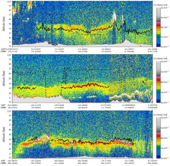
Figure 5 shows three examples of the resulting aerosol layer height derived from 1064 nm CALIOP measurements as previously described. The solid line indicates the effective aerosol layer height calculated using eq. (1), and the dashed line represents the aerosol layer height assumed in the pre-vious version of OMAERUV algorithm (Torres et al., 2007). CALIOP’s observed vertical structure of the aerosol load on 4 April 2007 near the Bodele depression in the central Sa-haran shows the unmistakable signature of a rising column of dust between the surface and about 3 km at 16◦N; 12◦E is shown in the top panel of Fig. 5. The airborne dust plume spreads north and south of the source in an atmospheric layer between 3 and 5 km. The aerosol layer height assumed in the OMAERUV algorithm is underestimated by as much as 2 km in relation to that inferred from CALIOP observations.
The center panel illustrates the vertical structure of a smoke layer as seen by the CALIPSO lidar on 12 August 2006 over Angola and Namibia, and the southern Atlantic Ocean. CALIOP observations show the westward flow of smoke from fires in Angola and Namibia over the southern Atlantic Ocean. The CALIOP curtain image shows a south-north transect of the smoke layer along the western coast of Central Africa from Angola, covering Angola’s coastal waters (∼12◦S; 13◦E), and reaching land again over the Democratic Republic of the Congo’s coastal area (∼5◦S, 11.5 E). Over the central and northern sections of the tran-sect, the aerosol layer is clearly located above low clouds. The smoke layer over land generated from fires in Angola and Namibia occupies a 2.5 km thick layer that goes from the surface (about 1 km above sea level) to 3.5 km as indicated by the attenuated backscatter signal. The assumed aerosol layer height is consistently higher than the CALIOP derived value. A layer of carbonaceous aerosols as seen by the OMI and CALIOP sensors over central Brazil on 30 September 2007 is depicted on the bottom panel of Fig. 5. The CALIOP curtain plot depicts the vertical structure of the layer over a region between 10◦S and 30◦S along CALIOPS’s orbital track. On
the northernmost end of the plume, the aerosol load is located in a 1 km-thick layer between 3 and 4 km above the ground, and widens towards the south. In general, the assumed height is about 1 km higher than the CALIOP-based estimate.
4.4 CALIOP-based aerosol height climatology
The procedure described in the previous section to derive an effective aerosol layer height was applied to the global CALIOP record over the 30 month period from July 2006 to December 2008. The extension beyond 2008 was hindered by the loss of the OCCP resulting from the onset of the OMI row anomaly discussed in Sect. 2. Gridded 1◦×1◦ res-olution monthly averages of ALH were calculated. A min-imum of five data points per grid were required to produce a monthly value. Extracts from a degraded 5◦×5◦ gridded
product were used to fill gaps in the original 1◦×1◦
prod-uct resulting from CALIOP’s lack of global coverage and the interference of clouds. Additionally, image processing tech-niques using convolution and Gaussian smoothing (Gonzalez and Woods, 1992) were applied to reduce the noise and min-imize the effect of isolated maxima and minima.
Figure 6 shows global maps of the monthly averaged aerosol layer height (Zclp), in km above surface, derived from
CALIOP observations. Maps shown correspond to the mid-season months (January, April, July, October).
TheZclpspatial distribution in January is dominated by the
presence of desert dust and carbonaceous aerosols copiously produced by their emission sources in the Saharan (desert dust) and equatorial Africa (biomass burning). Zclp values
between 3 and 4 km predominate over the northern African deserts, while values between 2 and 3 km are observed asso-ciated with the fire activity in the tropical belt along the At-lantic coast from Guinea to Nigeria, and extending eastwards to Ethiopia. Over the northern Atlantic Ocean,Zclpdescends
rapidly westwards from over 2 km at the North African west coast to the 45◦W meridian, and continues to decrease, with some oscillations, to minimum values of about 1 km over the Gulf of Mexico. Zclp values around 3 km can be observed
over the SE United States as a consequence of local fires, as well as long-range transport from Central America. High Zclp values are also observed in the Southern Hemisphere
summer over the land masses of South America (Patagonia), West Africa, and Australia where desert dust production and smoke from brush fires (Australia) are commonly observed in January.
A significant narrowing in theZclpnorth–south
distribu-tion over the Atlantic Ocean is apparent in April following the conclusion of the equatorial Africa biomass-burning sea-son. Zclp values higher than those observed in winter are
Fig. 5. CALIOP-measured 1064 nm backscatter profiles for three aerosol events: desert dust layer over central Saharan (top); smoke layer over Angola and Namibia (middle); smoke layer over central Brazil (bottom). CALIOP-based (solid line) and previously assumed (dashed line) aerosol layer heights are shown.
and local sources, as well as contribution from transport from Mexico and Central America (southeast). The ob-served Zclp values lower than 3 km over the western half
of the US are likely associated with local dust produc-tion. As a consequence of the activation of dust sources in Central Asia, elevated layers (3 km and higher) are appar-ent over Afghanistan, Turkmenistan, and Uzbekistan. Long-range transport of desert dust from the Saharan sources across the Mediterranean, and from sources in Central Asia trigger the spread of dust aerosol layers about 2.5 km high over western and northern Europe. Eastward transport of desert dust following the spring activation of the Gobi and Taklamakan deserts, and layers of carbonaceous aerosols from biomass burning in Southeast Asia linger over East Asia in layers 2 to 3 km high.
An enhanced July Zclp, associated with the northward
spread of aerosol layers from boreal fires in Canada and Siberia, is observed at about 3 km over northern Canada and the Arctic. The summer Saharan aerosol layer over the Atlantic Ocean between 10◦N and 30◦N varies in altitude between 3.5–4.0 km at the west coast of North Africa go-ing down towards the west, reachgo-ing 1.5 km over the Gulf
of Mexico. Smoke from biomass-burning activity in Central Africa spills over the southern Atlantic Ocean in an aerosol layer at 2–2.5 km.
The October global aerosol height distribution is char-acterized by an overall Zclp decrease. Except for a height
increase over the biomass-burning regions in the Southern Hemisphere, autumnZclpvalues are lower than the previous
season values by 1–2 km over most of the globe. The Sa-haran layer Zclp over the Atlantic Ocean reaches values as
low as 1.5 km about halfway between North Africa and the Gulf of Mexico. The carbonaceous aerosol layer, known as the “river of smoke”, flowing off Southeast Africa along the Indian Ocean at a 1–2 km heightZclpis clearly observed.
A global three-dimensional representation of the atmo-spheric aerosol load from multi-year CALIOP observations has recently been made available (Winker et al., 2013). A global seasonal description of aerosol height is presented in Fig. 9 of Winker et al. (2013), defined as the altitude at which 63 % of the AOD lies below (H63). Although the
Fig. 6. Monthly average aerosol layer height.
Fig. 7. Evaluation of AOD retrieval using standard aerosol layer height assumption (left) and CALIOP climatology (right) at the Banizoumbou site.
over the South Atlantic) can also be identified in Winker et al. (2013), a direct comparison between the two products is not meaningful as they are essentially a representation of dif-ferent aspects of the aerosol vertical distribution. TheH63
parameter represents the height at which about two thirds of the total aerosol load lies below, whereasZclpis a measure
of the level of peak absorbing aerosol concentration. TheH63
value is calculated including all aerosol types, whereasZclp
was specifically designed to capture the height of absorbing aerosol layers. Other important differences include time of observation (nighttime forH63and daytime forZclp) as well
as different wavelength which, as discussed in this work, may produce different height results in the presence of carbona-ceous aerosols.
5 Evaluation of improvements in OMAERUV retrievals
A brief discussion of the effect of the algorithm upgrades on retrieved products is presented here. Comprehensive assess-ments of the OMAERUV products using ground-based and other satellite observations are discussed in detail by Ahn et al. (2013) and Jethva et al. (2013).
The effect of using the CALIOPZclpclimatology as
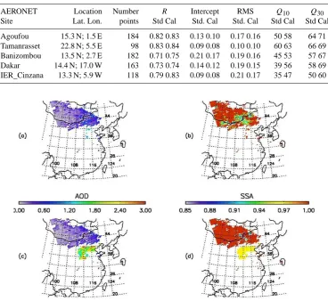
in-put in the OMI inversion algorithm was evaluated by com-paring the optical depth from the OMAERUV algorithm to AERONET observations (Holben et al., 1998) using both the standard algorithm aerosol height assumption and the aerosol altitude extracted from the CALIOP climatology de-scribed here. The assessment exercise was carried out us-ing AERONET measurements at the five sites listed in Ta-ble 1, where the presence of elevated dust and smoke lay-ers is routinely observed. OMAERUV AOD retrievals within a radius of 40 km of the AERONET site were compared to ground-based observations within a±10 min window (Ahn et al., 2013). Columns 4 through 8 in Table 1 show respec-tively the resulting correlation coefficient (r), intercept, the rms, and the number of retrievals within 10 % (Q10) and
30 % (Q30) of the AERONET values, for both the
Table 1. Summary statistics of OMAERUV and AERONET aerosol optical depth comparison.
AERONET Location Number R Intercept RMS Q10 Q30
Site Lat. Lon. points Std Cal Std. Cal Std. Cal Std Cal Std Cal
Agoufou 15.3 N; 1.5 E 184 0.82 0.83 0.13 0.10 0.17 0.16 50 58 64 71
Tamanrasset 22.8 N; 5.5 E 98 0.83 0.84 0.09 0.08 0.10 0.10 60 63 66 69
Banizombou 13.5 N; 2.7 E 182 0.71 0.75 0.21 0.17 0.19 0.16 45 53 57 67
Dakar 14.4 N; 17.0 W 163 0.73 0.74 0.14 0.12 0.19 0.15 39 56 58 69
IER_Cinzana 13.3 N; 5.9 W 118 0.79 0.83 0.09 0.08 0.21 0.17 35 47 50 60
Fig. 8. Retrieved AOD and SSA at 388 nm from the previous (a, b) and improved (c, d) OMI UV algorithm over northeastern China on 20 August 2007.
approach yields higher correlation coefficients (between 0.74 and 0.84) and slightly smaller intercepts. The improvement is noticeable in terms of the Q10 andQ30 parameters,
de-fined as the number of points (in percent) within 10 % and 30 % of the ground truth observations.Q10went up between
3 and 17 % at the five sites whereasQ30increased between
3 % and 11 %. In most cases the effect of using the CALIOP-based aerosol layer height was to reduce AERONET-OMI differences in the winter season when the aerosol layer height is underestimated by the standard assumption. The observed improvement is smallest in the middle of the Sa-haran (Tamanrasset site) and increases rapidly away from the dust aerosol source areas with the largest improvement registered at Dakar. The scatter plot in Fig. 7 illustrates the resulting OMAERUV AOD improvement in relation to AERONET observations at the Banizoumbou AERONET site.
As illustrated in Fig. 3, the use of CO measurements as an aerosol tracer has facilitated the identification of carbona-ceous aerosols over arid regions, where the distinction
be-tween dust and smoke particles would not have been possi-ble without the availability of CO observations. The AIRS CO data has also enabled the detectability and characteriza-tion of high levels of boundary layer pollucharacteriza-tion aerosols unde-tectable by the previous OMAERUV algorithm without the help of AIRS CO data. Figure 8 depicts the retrieved fields of aerosol optical and single scattering albedo on 20 Au-gust 2007 over northeastern China by the previous (top) and current (bottom) versions of the algorithm. Previously unde-tected aerosol load (AOD > 1.0, SSA∼0.97) is apparent over Beijing, extending over a large area west and southwest of the city. These are likely pollution aerosols in the boundary layer.
6 Summary and conclusions
OMAERUV algorithm. The combined use in real time of ob-servations from OMI and AIRS on two different satellites is only possible thanks to the near-simultaneity of A-train ob-servations.
It has been shown that the combined use of AIRS CO ob-servations and the OMI UV aerosol index provides a way of reliably identifying the absorbing aerosol type when absorb-ing aerosols have been positively detected via the AI. Be-cause CO is an excellent tracer of carbonaceous aerosols, el-evated values of both AI and CO correspond in most cases to the presence of smoke layers, whereas the occurrence of high AI values and low CO amounts are associated with layers of desert dust aerosols. Another useful application of the AIRS CO data is the identification of high boundary layer aerosol loads that would otherwise be dismissed as cloud contami-nation by OMAERUV. Because of the large aerosol load as-sociated with these events over biomass-burning regions and eastern China, it is possible to retrieve both aerosol optical depth and single scattering albedo.
We made use of time- and space-collocated CALIOP and OMI observations for the determination of the height of el-evated layers of carbonaceous and desert dust aerosols de-tected by OMI’s near-UV observations. An effective aerosol layer height was calculated as the attenuated-backscatter-weighted average height obtained from CALIOP’s 1064 nm measurements. Observations at 1064 nm were chosen over the 532 nm measurements because of apparent saturation ef-fects at the shorter wavelength. The OMI-CALIOP combined analysis was carried out over a 30-month record from July 2006 to December 2008. In early 2009 instrumental issues affecting the OMI sensor resulted in the loss of the colloca-tion capability.
A 30-month climatology of aerosol layer height was cal-culated. The impact of using CALIOP-based climatology of aerosol layer height was evaluated by comparing OMI-retrieved AODs to AERONET observations at a number of locations in North Africa. Validation results indicate that although previous algorithm assumptions on aerosol layer height worked reasonably well, the use of the CALIOP-based climatology produces a noticeable improvement of re-trieval results. The CALIOP-based absorbing aerosol layer height climatology and the real-time use of AIRS CO obser-vations have been integrated into the current version of the OMAERUV algorithm.
Acknowledgements. We thank the AIRS and CALIOP projects for producing and making available the data sets used in this analysis. We also thank the AERONET project and the Principal Investiga-tors of the sites used in this work. We gratefully acknowledge the anonymous reviewers whose feedback contributed to improve the manuscript.
Edited by: A. Kokhanovsky
References
Ahn, C., Torres, O., and Jethva, H.: Assessment of OMI near UV Aerosol Optical Depth over Land, J. Geophys. Res., submitted, 2013.
Ahn C., Torres, O., and Bhartia, P. K.: Comparison of OMI UV Aerosol Products with Aqua-MODIS and MISR observations in 2006, J. Geophys. Res, 113, D16S27, doi:10.1029/2007JD008832, 2008.
Anderson, T. L., Charlson, R. J., Bellouin, N., Boucher, O. , Chin, M., Christopher, S. A., Haywood, J. , Kaufman Y. J., Kinne, S., Ogren, J. A., Remer, L. A., Takemura, T., Tanre, D., Torres, O., Trepte, C. R., Wielicki, B. A., Winker, D. M., and Yu, H.: Am “A-Train” Strategy for Quantifying Direct Climate Forcing by Anthropogenic Aerosols, Bull. Amer. Met. Soc., 86, 1795–1809, doi:10.1175/BAMS-86-12-1795, 2005.
Andreae, M. O., Anderson, B. E., Blake, D. R., Bradshaw, J. D., Collins, J. E., Gregory, G. L., Sachse, G. W., and Shipham, M. C.: Influence of plumes from biomass burning on atmospheric chemistry over the equatorial and tropical South Atlantic during CITE 3, J. Geophys. Res., 99, 12793–12808, 1994.
Andreae, M. O. and Metlet, P.: Emission of trace gases and aerosols from biomass burning, Global Biogeochem. Cy., 15, 955–966, 2001.
Angstrom, A.: On the atmospheric transmission of Sun radiation and on dust in the air, Geogr. Ann., 12, 130–159, 1929. Aumann, H. H., Chahine, M. T., Gautier, C., Goldberg, M. D.,
Kalnay, E., McMillin, L. M., Revercomb, H., Rosenkranz, P. W., Smith, W. L., Staelin, D. H., Strow, L. L., and Susskind, J.: AIRS/AMSU/HSB on the Aqua mission, Design, science objectives, data products, and processing systems, IEEE Trans. Geosci. Remote Sens., 41, 253–264, 2003.
Chahine, M. T.: Remote sounding of cloudy atmospheres, I, The single cloud layer, J. Atmos. Sci., 31, 233–243, 1974.
Chen, Z., Torres, O., McCormick, M. P., Smith, W., and Ahn, C.: Comparative study of aerosol and cloud detected by CALIPSO and OMI, Atmos. Environ., 51, 187–195, 2012.
De Graaf, M., Stammes, P., Torres, O., and Koelemeijer, R. B. A.: Absorbing Aerosol Index: Sensitivity Analysis, Application to GOME and Comparison with TOMS, J. Geophys. Res., 110, D01201, doi:10.1029/2004JD005178, 2005a.
De Graaf, M. and Stammes, P.: SCIAMACHY Absorbing Aerosol Index – calibration issues and global results from 2002–2004, At-mos. Chem. Phys., 5, 2385–2394, doi:10.5194/acp-5-2385-2005, 2005.
Penning de Vries, M. J. M., Beirle, S., and Wagner, T.: UV Aerosol Indices from SCIAMACHY: introducing the SCattering Index (SCI), Atmos. Chem. Phys., 9, 9555–9567, doi:10.5194/acp-9-9555-2009, 2009.
Dirksen, R. J., Folkert Boersma, K., de Laat, J., Stammes, P., van der Werf, G. R., Val Martin, M., and Kelder, H. M.: An aerosol boomerang: Rapid around-the-world transport of smoke from the December 2006 Australian forest fires observed from space, J. Geophys. Res., 114, D21201, doi:10.1029/2009JD012360, 2009. Dubovik, O., Holben, B., Eck, T. F., Smirnov, A., Kaufman, Y. J., King, M. D., Tanre, D., and Slutsker, I.: Variability of absorption and optical properties of key aerosol types observed in world-wide locations, J. Atm. Sci., 59, 590–608, 2002.
of the optical depth of biomass burning, urban and desert dust aerosols, J. Geophys. Res., 104, 31333–31349, 1999.
Edwards D. P., Emmons, L. K., Hauglustaine, D. A., Chu, D. A., Gille, J. C., Kaufman, Y. J., Petron, G., Yurganov, L. N., Giglio, L., Deeter, M. N., Yudin, V., Ziskin, D. C., Warner, J., Lamarque, J. F., Francis, G. L., Ho, S. P., Mao, D., Chen, J., Grechko, E. I., and Drummond, J. R.: Observations of carbon monoxide and aerosols from the Terra satellite: Northern Hemisphere variabil-ity, J. Geophys. Res., 109, D24202, doi:10.1029/2004JD004727, 2004.
Edwards, D. P., Emmons, L. K., Gille, J. C., Chu, A., Attie, J.-L., Giglio, L., Wood, S. W., Haywood, J., Deeter, M. N., Massie, S. T., Ziskin, D. C., and Drummond, J. R.: Satelliteobserved pol-lution from Southern Hemisphere biomass burning, J. Geophys. Res., 111, D14312, doi:10.1029/2005JD006655, 2006.
Ginoux, P., Chin, M., Tegen, I., Prospero, J. M., Holben, B., Dubovik, O., and Lin, S.-J.: Sources and distributions of dust aerosols simulated with the GOCART model, J. Geophys. Res., 106, 20255–20273, doi:10.1029/2000JD000053, 2001.
Gleason, J., Hsu, N.C., and Torres, O.: Biomass burning smoke measured using backscattered ultraviolet radiation: SCARB and Brazilian smoke inter annual variability, J. Geophys Res., 103, 31969–31978, 1998.
Gonzalez, R. and Woods, R.: Digital Image Processing, Addison-Wesley Publishing Company, 192 pp., 1992.
Hair, J. W., Hostetler, C. A., Cook, A. L., Harper, D. B., Fer-rare, R. A., Mack, T. L., Welch, W., Isquierdo, L. R., and Hovis, F. E.: Airborne high spectral resolution lidar for pro-filing aerosol optical properties, Appl. Optics, 47, 6734–6752, doi:10.1364/AO.47.006734, 2008.
Herman, J. R., Bhartia, P. K., Torres, O., Hsu, C., Seftor, C., and Celarier, E.: Global Distribution of UVabsorbing Aerosols From Nimbus7/TOMS data, J. Geophys. Res., 102, 16911–16922, 1997.
Herman, J. R., and Celarier, E.: Earth surface reflectivity climatol-ogy at 340 and 380 nm from TOMS data, J. Geophys. Res., 102, 28003–28011, 1997.
Holben, B. N., Eck, T. F., Slutsker, I., Tanre, D., Buis, J. P., Set-zer, A., Vermote, E., Reagan, J. A., Kaufman, Y. J., Nakajima, T., Lavenu, F., Jankowiak I.„ and Smirnov, A.: AERONET – A federated instrument network and data archive for aerosol char-acterization, Remote Sens. Environ., 66, 1–16, 1998.
Hsu, N. C., Herman, J. R., Bhartia, P. K., Seftor, C. J., Thompson, A.M., Gleason, J. F., Eck, T. F., and Holben, B. N.: Detection of biomass burning smoke from TOMS measurements, Geophys. Res. Lett., 23, 745–748, 1996.
Jethva, H., Torres, O., and Ahn, C.: Global Assessment of OMI Aerosol Single-scattering Albedo in Relation to Ground-based AERONET Inversion, J. Geophys. Res., submitted, 2013. Jethva, H. and Torres, O.: Satellite-based evidence of
wavelength-dependent aerosol absorption in biomass burning smoke inferred from Ozone Monitoring Instrument, Atmos. Chem. Phys., 11, 10541–10551, doi:10.5194/acp-11-10541-2011, 2011.
Kacenelenbogen, M., Vaughan, M. A., Redemann, J., Hoff, R. M., Rogers, R. R., Ferrare, R. A., Russell, P. B., Hostetler, C. A., Hair, J. W., and Holben, B. N.: An accuracy assess-ment of the CALIOP/CALIPSO version 2/version 3 daytime aerosol extinction product based on a detailed multi-sensor,
multi-platform case study, Atmos. Chem. Phys., 11, 3981–4000, doi:10.5194/acp-11-3981-2011, 2011.
Levelt, P. F., Hilsenrath, E., Leppelmeier, G. W., van den Ooord, G. H. J., Bhartia, P. K., Taminnen, J., de Haan, J. F., and Veefkind, J. P.: Science objectives of the Ozone Monitoring Instrument, IEEE Trans. Geosci. Remote Sens., 44, 1093–1101, 2006.
Levy, R. C., Remer, L. A., Kleidman, R. G., Mattoo, S., Ichoku, C., Kahn, R., and Eck, T. F.: Global evaluation of the Collection 5 MODIS dark-target aerosol products over land, Atmos. Chem. Phys., 10, 10399–10420, doi:10.5194/acp-10-10399-2010, 2010. Loveland, T. R., Reed, B. C., Brown, J. F., Ohlen, D. O., Zhu, Z., Yang, L., and Merchant, J. W.: Development of a global land cover characteristics database and IGBP DISCover from 1 km AVHRR data. Int. J. Remote Sens., 21, 1303–1330, 2000. Luo, M., Boxe, C., Jiang, J., Nassar, R., and Livesey, N.:
Interptation of Aura satellite observations of CO and aerosol index re-lated to the December 2006 Australia fires, Remote Sens. Envi-ron., 114, 2853–2862, 2010.
McMillan, W. W., Barnet, C., Strow, L., Chahine, M. T., McCourt, M. L., Warner, J. X., Novelli, P. C., Korontzi, S., Maddy, E. S., and Datta, S.: Daily global maps of carbon monoxide from NASA’s Atmospheric Infrared Sounder, Geophys. Res. Lett., 32, L11801, doi:10.1029/2004GL021821, 2005.
Pan, L., Guille, J. C., Edwards, D. P., and Bailey, P. L.: Retrieval of tropospheric carbon monoxide for the MOPITT experiment, J. Geophys. Res., 103, 32277–32290, 1998.
Savtchenko A., Kummerer, R., Smith, P., Gopalan, A., Kempler, S., and Leptoukh, G., A-Train Data Depot: Bringing Atmospheric Measurements Together, IEEE Trans. Geos. Rem. Sens., 46, 2788–2795, 2008.
Seftor, C. J., Hsu, N. C., Herman, J. R., Bhartia, P. K., Torres, O., Rose, W. I., Schneider, D. J., and Krotkov, N.: Detection of vol-canic ash clouds from Nimbus7/total ozone mapping spectrome-ter, J. Geophys. Res., 102, 749–759, 1997.
Sinha, P., Hobbs, P. V., Yokelson, R. J., Bertschi, I. T., Blake, D. R., Simpson, I. J., Gao, S., Kirchstetter, T. W., and No-vakov, T.: Emissions of trace gases and particles from sa-vanna fires in southern Africa, J. Geophys. Res., 108, 8487, doi:10.1029/2002JD002325, 2003.
Susskind, J., Barnet, C. D., and Blaisdell, J. M.: Retrieval of atmo-spheric and surface parameters from AIRS/AMSU/HSB data in the presence of clouds, IEEE Trans. Geosci. Remote Sens., 41, 390–409, 2003.
Toledano, C., Wiegner, M., GROß, S., Freudenthaler, V., Gasteiger, J., Muller, D., Schladitz, A., Weinzierl, B., Torres, B., and O’Neill, N. T.: Optical properties of aerosol mixtures from sun-sky radiometry during SAMUM-2, Tellus B, 63, 635–648, 2011. Torres O., Bhartia, P. K., Herman, J. R., and Ahmad, Z.: Derivation of aerosol properties from satellite measurements of backscat-tered ultraviolet radiation. Theoretical Basis, J. Geophys. Res., 103, 17099–17110, 1998.
Torres, O., Bhartia, P. K., Herman, J. R., Syniuk, A., Ginoux, P., and Holben, B.: A long term record of aerosol optical depth from TOMS observations D and comparison to AERONET measure-ments, J. Atm. Sci., 59, 398–413, 2002.
Turquety, S., Hurtmans, D., Hadji-Lazaro, J., Coheur, P.-F., Cler-baux, C., Josset, D., and Tsamalis, C.: Tracking the emission and transport of pollution from wildfires using the IASI CO re-trievals: analysis of the summer 2007 Greek fires, Atmos. Chem. Phys., 9, 4897–4913, doi:10.5194/acp-9-4897-2009, 2009 Winker, D. M., Pelon, J., and McCormick, M. P.: “The CALIPSO
mission: Spaceborne lidar for observation of aerosols and clouds”, Proc. SPIE, 4893, 1–11 pp., 2003.
Winker, D. M., Tackett, J. L., Getzewich, B. J., Liu, Z., Vaughan, M. A., and Rogers, R. R.: The global 3-D distribution of tro-pospheric aerosols as characterized by CALIOP, Atmos. Chem. Phys., 13, 3345–3361, doi:10.5194/acp-13-3345-2013, 2013. Witte, J. C., Douglass, A. R., da Silva, A., Torres, O., Levy, R.,
and Duncan, B. N.: NASA A-Train and Terra observations of the 2010 Russian wildfires, Atmos. Chem. Phys., 11, 9287–9301, doi:10.5194/acp-11-9287-2011, 2011.
Yokelson, R. J., Bertschi, I. T., Christian, T. J., Hobbs, P. V., Ward, D. E., and Hao, W. M.: Trace gas measurements in nascent, aged, and cloud-processed smoke from African savanna fires by air-borne Fourier transform infrared spectroscopy (AFTIR), J. Geo-phys. Res., 108, 8478, doi:10.1029/2002JD002322, 2003. Yurganov, L. N., McMillan, W. W., Dzhola, A. V., Grechko, E. I.,
Jones, N. B., and van der Werf, G. R.: Global AIRS and MO-PITT CO measurements: Validation, comparison, and links to biomass burning variations and carbon cycle, J. Geophys. Res., 113, D09301, doi:10.1029/2007JD009229, 2008.