Atmos. Meas. Tech., 6, 3597–3612, 2013 www.atmos-meas-tech.net/6/3597/2013/ doi:10.5194/amt-6-3597-2013
© Author(s) 2013. CC Attribution 3.0 License.
Atmospheric
Measurement
Techniques
Open Access
Contrail study with ground-based cameras
U. Schumann1, R. Hempel2, H. Flentje3, M. Garhammer4, K. Graf1, S. Kox1, H. Lösslein4, and B. Mayer4 1Deutsches Zentrum für Luft- und Raumfahrt, Institut für Physik der Atmosphäre, Oberpfaffenhofen, Germany 2Deutsches Zentrum für Luft- und Raumfahrt, Simulations- und Softwaretechnik, Cologne, Germany
3Deutscher Wetterdienst, Meteorologisches Observatorium Hohenpeissenberg, Hohenpeissenberg, Germany 4Meteorologisches Institut, Ludwig-Maximilians-Universität, Munich, Germany
Correspondence to: U. Schumann ([email protected])
Received: 7 August 2013 – Published in Atmos. Meas. Tech. Discuss.: 19 August 2013 Revised: 25 November 2013 – Accepted: 26 November 2013 – Published: 20 December 2013
Abstract. Photogrammetric methods and analysis results for
contrails observed with wide-angle cameras are described. Four cameras of two different types (view angle<90◦ or whole-sky imager) at the ground at various positions are used to track contrails and to derive their altitude, width, and hor-izontal speed. Camera models for both types are described to derive the observation angles for given image coordinates and their inverse. The models are calibrated with sightings of the Sun, the Moon and a few bright stars. The methods are applied and tested in a case study. Four persistent con-trails crossing each other, together with a short-lived one, are observed with the cameras. Vertical and horizontal po-sitions of the contrails are determined from the camera im-ages to an accuracy of better than 230 m and horizontal speed to 0.2 m s−1. With this information, the aircraft causing the contrails are identified by comparison to traffic waypoint data. The observations are compared with synthetic camera pictures of contrails simulated with the contrail prediction model CoCiP, a Lagrangian model using air traffic move-ment data and numerical weather prediction (NWP) data as input. The results provide tests for the NWP and contrail models. The cameras show spreading and thickening con-trails, suggesting ice-supersaturation in the ambient air. The ice-supersaturated layer is found thicker and more humid in this case than predicted by the NWP model used. The simu-lated and observed contrail positions agree up to differences caused by uncertain wind data. The contrail widths, which depend on wake vortex spreading, ambient shear and turbu-lence, were partly wider than simulated.
1 Introduction
Contrails are linear clouds often visible to ground observers behind cruising aircraft. The conditions under which con-trails form (at temperatures below the Schmidt–Appleman criterion) and persist (at ambient humidity exceeding ice sat-uration) are well known (Schumann, 1996). The dynamics of young contrails depend on aircraft emissions and wake prop-erties and the pattern of contrails changes over their lifetime (Lewellen and Lewellen, 1996; Sassen, 1997; Mannstein et al., 1999; Jeßberger et al., 2013). Though contrails have been investigated for some time, still little is known about the full life cycle of individual contrails (Mannstein and Schumann, 2005; Heymsfield et al., 2010; Unterstrasser and Sölch, 2010; Graf et al., 2012; Minnis et al., 2013; Schumann and Graf, 2013).
3598 U. Schumann et al.: Contrail camera observations
Wide-angle digital cameras have been used before to ob-serve clouds (e.g., Seiz et al., 2007) and contrails (Sassen, 1997; Feister and Shields, 2005; Stuefer et al., 2005; Atlas and Wang, 2010; Feister et al., 2010; Mannstein et al., 2010; Shields et al., 2013). Whole-sky imagers using a fisheye lens image the full sky down, or nearly down, to the hori-zon (Shields et al., 2013). More narrow wide-angle cameras cover only part of the sky but with higher resolution. Besides color cameras, multispectral cameras recording in several spectral wavebands are also available (Feister and Shields, 2005; Seiz et al., 2007; Shields et al., 2013). Camera obser-vations often reveal interesting cloud properties, but a single camera is insufficient to determine the distance of an observ-able object (LeMone et al., 2013). A video scene from a sin-gle camera allows determining the angular but not the linear cloud speed. Horizontal contrail positions can be estimated if the contrail altitude is known from other sources (Atlas and Wang, 2010). A network of cameras has been used for observations of upper atmosphere clouds (Baumgarten et al., 2009) and other objects (Shields et al., 2013).
In regions with dense air traffic, the sky is often full of contrails, and the assignment of individual observed contrails to specific aircraft requires accurate contrail altitudes besides traffic information. The analysis of aged contrails requires the trajectory analysis from aircraft flight routes to contrail positions.
Here, we report on a case study where we observed con-trails with four wide-angle cameras, placed several kilome-ters apart and oriented at fixed positions in the sky, providing digital images every 10 s. If the same cloud detail could be identified in overlapping areas of stereo images taken with at least two cameras simultaneously, its three-dimensional posi-tion could be determined (Seiz et al., 2007). In our case, the horizontal distance between the cameras was too large for simultaneous observations, but cloud features moving with about constant speed across the camera view-fields could be used for photogrammetric analysis. The results are used to identify the causing aircraft, contrail positions vs. time with respect to NWP data, and to deduce contrail and atmospheric properties. For a direct comparison of simulated contrails with camera observations, we map the computed contrails on synthetic camera images. This requires algorithms which compute spherical coordinates for given pixel coordinates and their inverse.
The pixel positions of identifiable objects in digital camera images can be determined with standard image processing software. However, images of wide-angle cameras usually are distorted considerably (Weng et al., 1992; Garcia et al., 1997). In our case the distortion becomes obvious because straight contrails appear increasingly curved when coming close to the camera position, in particular near the edge of the camera image. The mathematical algorithm which de-scribes the transformation of image coordinates into horizon-tal spherical coordinates or vice versa, including corrections for distortion is called a camera model.
Camera models have been used widely for astronomical observations, mainly for dark sky imaging, e.g., for meteor trace analysis (Oberst et al., 2004), also for gravity wave analysis in mesospheric airglow images (Garcia et al., 1997), noctilucent cloud observations (Baumgarten et al., 2009), cloud mapping using calibration with stars and aircraft with known positions (Seiz et al., 2007; Shields et al., 2013), or for automatic identification of stars in digital images (Klaus et al., 2004).
In contrast to stars, cloud features are more fuzzy and vari-able in time, and hence only allow less accurate geomet-ric observations. Contrail features cover typically observa-tion angles of one or a few degrees. Therefore, our cam-era model uses a simplified imaging geometry and distortion model and exploits symmetry assumptions to cover the full image frame.
This article describes camera models for two types of wide-angle cameras (a whole-sky imager and a more narrow one). The camera models correct for radial distortion inside the camera and for the orientation of the camera with respect to the horizontal coordinate system. The camera models are calibrated by using observations of the Sun, the Moon, plan-ets and a few bright stars and landmarks. Moreover, we report results from aircraft track and contrail motion analysis with the camera models, and compare them with air traffic move-ment data, numerical weather prediction data, and simula-tions of contrail trajectories and spreading with a Lagrangian contrail model.
2 Camera models
2.1 The cameras used
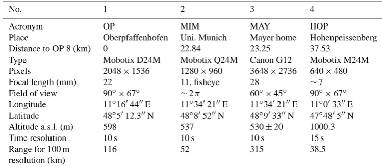
Cloud images were obtained in this study with four commer-cial digital video color cameras (Table 1). Photogrammetric analysis is described in detail for two of them (Figs. 1 and 2): 1. A wide-angle camera of type Mobotix D24M with L22 lens, installed on the roof of the Institute of Atmo-spheric Physics of the Deutsches Zentrum für Luft-und Raumfahrt (DLR, German Aerospace Center) at Oberpfaffenhofen (OP). The wide-angle lens covers a limited field of view and faces roughly westward with some upward tilting.
2. A whole-sky fisheye camera of type Mobotix Q24M installed on the roof of the Meteorological Insti-tute of the Ludwig-Maximilians-Universität in Munich (MIM), pointing vertically.
U. Schumann et al.: Contrail camera observations 3599
Table 1. The cameras.
No. 1 2 3 4
Acronym OP MIM MAY HOP
Place Oberpfaffenhofen Uni. Munich Mayer home Hohenpeissenberg
Distance to OP 8 (km) 0 22.84 23.25 37.53
Type Mobotix D24M Mobotix Q24M Canon G12 Mobotix M24M
Pixels 2048×1536 1280×960 3648×2736 640×480
Focal length (mm) 22 11, fisheye 28 ∼7
Field of view 90◦×67◦ ∼2π 60◦×45◦ 90◦×67◦
Longitude 11◦1604400E 11◦3402100E 11◦3402100E 11◦003300E
Latitude 48◦5012.300N 48◦805200N 48◦903300N 47◦480500N
Altitude a.s.l. (m) 598 537 530±20 1000.3
Time resolution 10 s 10 s 10 s 15 s
Range for 100 m 116 52 315 38.5
resolution (km)
2.2 Camera model algorithms
The camera model provides the relationship between celes-tial azimuth and elevation angle coordinates (A,E) and pixel coordinates (X, Y).X counts image columns from left to right, from 1 to 2048 and 1 to 1280, for camera 1 and 2, respectively;Y counts image rows from top to bottom, 1 to 1536 and 1 to 960. The azimuth Avaries from 0 to 360◦ (0◦: North; 90◦: East). The elevation is zero at the horizon and 90◦at the zenith. The algorithm makes use of the pixel and celestial coordinates of the camera midpoints, (X0,Y0, A0, E0). For camera 1, the coordinatesX0 andY0 are set to the midpoint of the image plane and the anglesA0andE0 are found from astronomical observations near this midpoint. For camera 2, the midpoint is set to coincide with the vertical direction (E=90◦,A=0◦) and the values of the coordinates X0andY0are found by minimizing the model residuals, i.e., the root mean square (rms) differences between observed and computed star observations. A large focal length of the cam-eras is important for high resolution (Table 1), but its value is not used explicitly in the models.
The camera model describes the mapping between pixel coordinates (X,Y) in the image and(X0, Y0)coordinates in an imaginary plane onto which the spherical object coordi-nates (A,E) are projected (the so-called projection plane). The two camera types differ in their mapping transformations (see Fig. 3). For camera 1, which is tilted upward, the projec-tion plane is the plane tangential to the celestial unit sphere, with the tangential point being at the image center. The rect-angular coordinates in this plane are defined by gnomonic projection. For camera 2, the lens projects the sky onto a hor-izontal finite circular image resolved by a rectangular set of image pixels. Here, we choose the horizontal plane as projec-tion plane, with the posiprojec-tion angle of an object’s projecprojec-tion point being its azimuth, and the center distance being propor-tional to its zenith distance angle. An affine transformation is constructed between the two Cartesian coordinate systems.
Fig. 1. Wide-angle camera in Oberpfaffenhofen (OP, left panel) and Munich (MIM, right panel). The sphere in
the top-cross of the St. Markus church, above the MIM camera, is used as southeastern landmark.
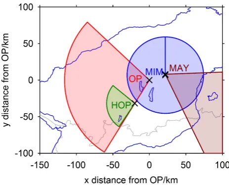
Fig. 2. Positions, view angles and view ranges of 100mresolution for the cameras Oberpfaffenhofen (OP), Mu-nich (MIM), private (MAY), and Hohenpeissenberg (HOP) in Southern Germany. MIM and MAY are 1.27km
apart, so nearly coincide in this figure. The region is located between Lake Constance (West), Chiemsee (East), Danube (North), and Inn (South). The lakes Ammersee and Starnberger See are within the range of MIM, south of Munich.
24
Fig. 1. Wide-angle camera in Oberpfaffenhofen (OP, left panel) and
Munich (MIM, right panel). The sphere in the top cross of the St. Markus church, above the MIM camera, is used as southeastern landmark.
Additionally, the camera model accounts for the distor-tion caused by the camera lens, i.e., its deviadistor-tion from the ideal geometry of a so-called pinhole camera (van de Kamp, 1967). We assume that radial lens distortions are symmetric with respect to rotation around the image center. Instead of a polynomial function (e.g., Weng et al., 1992), we use an exponential function because of well-defined asymptotic be-havior for small and large radius arguments.
3600 U. Schumann et al.: Contrail camera observations
over-determined, least-square fits are applied in the param-eter computations for both the distortion function and the affine transformation.
Based on these considerations, the forward transformation
(A, E)=f (X, Y ) (1)
is constructed as follows:
1. The camera pixels (X,Y) are transformed into rectan-gular coordinates (xd,yd) relative to the camera center, withydpointing upwards in the image,
xd=X−X0, yd=Y0−Y. (2)
2. The coordinates (xd,yd) are mapped to (x0,y0) assum-ing a radially symmetric image distortion,
rd= q
xd2+yd2, r=a rd(1+bexp(crd)). (3) The ratior/rdof the radii, with coefficientsa >0,b≥ 0,c >0, is used to correct for radial distortion,
x0=xdr/rd, y0=ydr/rd. (4)
3. The rectified image coordinates (x0, y0) are mapped with an affine transformation to projection plane co-ordinates (X0, Y0) which accounts (as discussed in Sect. 2.3) for camera inclinations and rotations (pa-rameters Bˆ, andDˆ), horizontal shifts (parametersCˆ, andFˆ) and scaling (parameters Aˆ, andEˆ), possibly different in the two directions,
X0= ˆAx0+ ˆBy0+ ˆC, Y0= ˆDx0+ ˆEy0+ ˆF, (5)
R=pX02+Y02. (6)
4. For camera 1, the projection plane coordinates (X0,Y0) are related to the angles (A,E) by trigonometry (van de Kamp, 1967):
sin(E)=sin(E0)+Y
0cos(E
0) √
1+R2 , (7)
cos(A−A0)=
tan(E)cos(E0)−Y0sin(E0) sin(E0)+Y0cos(E0)
, (8)
sin(A−A0)=
X0tan(E) sin(E0)+Y0cos(E0)
. (9)
For camera 2, we use:
E=90◦(1−R), cos(A)=Y0/R,
sin(A)=X0/R. (10)
5. Finally, equations sin(A0)=SA, cos(A0)=CA, with givenSA,CA, imply ifCA>0:A0=sin−1(SA), else: A0=180◦−sin−1(SA). Negative values of Aare in-cremented by 360◦.
Fig. 1. Wide-angle camera in Oberpfaffenhofen (OP, left panel) and Munich (MIM, right panel). The sphere in
the top-cross of the St. Markus church, above the MIM camera, is used as southeastern landmark.
Fig. 2. Positions, view angles and view ranges of 100mresolution for the cameras Oberpfaffenhofen (OP), Mu-nich (MIM), private (MAY), and Hohenpeissenberg (HOP) in Southern Germany. MIM and MAY are 1.27km
apart, so nearly coincide in this figure. The region is located between Lake Constance (West), Chiemsee (East),
Danube (North), and Inn (South). The lakes Ammersee and Starnberger See are within the range of MIM, south
of Munich.
24
Fig. 2. Positions, view angles and view ranges of 100 m
resolu-tion for the cameras Oberpfaffenhofen (OP), Munich (MIM), pri-vate (MAY), and Hohenpeissenberg (HOP) in Southern Germany. MIM and MAY are 1.27 km apart, so nearly coincide in this figure. The region is located between Lake Constance (West), Chiemsee (East), Danube (North), and Inn (South). The lakes Ammersee and Starnberger See are within the range of MIM, south of Munich.
The inverse transformation
(X, Y )=F (A, E) (11)
is set up consistently as follows.
1. Camera 1 uses the gnomonic projection of the angles (A, E)to camera image coordinates(X0, Y0)(van de Kamp, 1967):
X0= cos(E)sin(A−A0)
sin(E)sin(E0)+cos(E)cos(E0)cos(A−A0)
, (12) Y0=sin(E)cos(E0)−cos(E)sin(E0)cos(A−A0)
sin(E)sin(E0)+cos(E)cos(E0)cos(A−A0)
, (13) R=
q
X02+Y02. (14)
Camera 2 uses the inverse of Eq. (10), R=(90◦−E)/90◦, X0=Rsin(A),
Y0=Rcos(A). (15)
For both cameras, we compute the inverse of Eq. (5): y0=
ˆ
D(X0− ˆC)+ ˆA(Fˆ−Y0) ˆ
BDˆ − ˆEAˆ , (16)
x0=(X0− ˆBy0− ˆC)/A,ˆ r= q
x02+y02. (17) The inverse solutionrd(r)of Eq. (3) is determined by a Newton iteration, starting from a first guessrd=r/a. Finally the pixel coordinates are given by
xd=x0rd/r, yd=y0rd/r, X=xd+X0,
U. Schumann et al.: Contrail camera observations 3601
In total, both cameras use 11 free model parameters: ˆ
A,B,ˆ C,ˆ D,ˆ E,ˆ Fˆ,a, b, c, E0, A0for camera 1, andX0, Y0 in-stead ofE0, A0for camera 2. To avoid a conflict in scaling byaand the Turner coefficients, we normalize the latter such that the determinantAˆEˆ− ˆBDˆ =1. This reduces the number of free parameters to 10. For their calibration, we assume that a set of observations(Ai, Ei, Xi, Yi), i=1,2, . . . , n, is avail-able (see Fig. 3). In the following we will show how these parameters are determined.
For each observation, we compute R(Ai, Ei) from Eqs. (2)–(6) andR(Xi, Yi)from Eqs. (12)–(15). Ideally, both should be equal. Here, we determine the fitting parameters a, b, centering Eq. (3) such that the differences have mini-mum rms values,
SR= n X
i
(R(Ai, Ei)−R(Xi, Yi))2. (19)
Using Eqs. (3) and (4), we computeri,xi0,y
0
ifor each ob-servation. Together with theXi0,Yi0 from above, these data should satisfy Eq. (5):
Xi0= ˆAxi0+ ˆByi0+ ˆC, Yi0= ˆDxi0+ ˆEyi0+ ˆF,
i=1,2, . . . , n, (20)
with unknownsA,ˆ B,ˆ C,ˆ D,ˆ E,ˆ Fˆ. This set of equations can be expressed in matrix notation as
Xi0=Jx ˆ A ˆ B ˆ C
, Yi0=Jy ˆ D ˆ E ˆ F
. (21)
Forn >3, Eq. (21) is over-determined. A least-square so-lution for the model parameters is found by solving the nor-mal equations,
JTxJx ˆ A ˆ B ˆ C
=JTx X
0
i
, JTyJy ˆ D ˆ E ˆ F
=JTy Y
0
i
. (22)
These linear systems with 3 unknowns each are solved nu-merically.
Optimal values ofA0, E0(camera 1) orX0, Y0(camera 2) are found when minimizing the properly weighted sums of the squared residuals of the observations for angles and pixel coordinates together with the radial residuals (Eq. 19). The camera models are available as implementations in MS Ex-cel 2010, Python, and Fortran, using various optimization al-gorithms (e.g., Schumann et al., 2012).
2.3 Camera calibration observations
For the determination of the camera model parameters (Ta-ble 2), we need a set of coordinates(Xi, Yi), i=1,2, . . . , n, related to known azimuth and elevation(Ai, Ei). Basically, n=3 linearly independent pairs of (precise) observations are
Fig. 3. Coordinate lines of mutual transformation for the two camera types (left panels: limited wide-angle,
right panels: whole-sky imager), and field coverage with astronomical sightings (circles) for camera type 1 (e.g. OP, left panels) and type 2 (MIM, right panesl) in image coordinates (X, Y, top panels) and celestial angle coordinates (A, E, bottom panels). The grey triangles denote landmark observations.
! "!
Fig. 4. Distribution of residuals in image (left panel) and angle (right panel) coordinates for camera 1 (OP, open
circles) and 2 (MIM, closed circles). Triangles denote landmark observations.
25
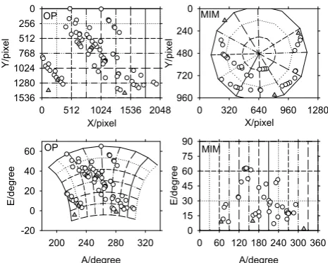
Fig. 3. Coordinate lines of mutual transformation for the two
cam-era types (left panels: limited wide-angle, right panels: whole-sky imager), and field coverage with astronomical sightings (circles) for camera type 1 (e.g., OP, left panels) and type 2 (MIM, right panels) in image coordinates (X, Y, top panels) and celestial angle coor-dinates (A, E, bottom panels). The grey triangles denote landmark observations.
sufficient to determine the 6 coefficients of the affine trans-formations (Eq. 5). At least 3 (partly the same) observations spaced over the radial range are needed to determine the 3 co-efficients in the radial distortion function (Eq. 3). However, to compensate for observation errors, a large set of observa-tions covering the whole field of view is desirable,n3.
Here, we describe calibration for cameras OP and MIM. For these cameras, we use occasional sightings of celestial objects in images taken at times with clear sky. Since the ori-entation of the cameras is fixed, sightings taken at different, accurately measured times can be used for a single camera model.
In the actual application, the field coverage is far from op-timal. One of the cameras was operated routinely only during daytime. Moreover, because of strong stray light at the urban observation positions, only a few usable nighttime observa-tions are available. Therefore, the cameras are calibrated us-ing observations of the Sun, Moon, and Vega for OP, and the Sun, Moon, Venus, Jupiter, and Sirius for MIM.
For these sightings, the coordinates of the brightest pixel are measured at high magnification using the software Ir-fanview. The planetarium software Guide 9.0 provides high-precision spherical coordinates with respect to the horizon, including the correction for atmospheric refraction, for the times when the digital images were taken.
3602 U. Schumann et al.: Contrail camera observations
closer to the lower-left corner. Measurements in the upper-right or lower-left image corner are missing. Observations of landmarks at low elevation angles at distances between 130 and 360 m are used for independent model tests (see Fig. 4). For MIM, observations are available mainly in the South. The northern range of azimuth angles between 292◦and 72◦ is not covered. Three landmarks at low elevation angles at distances between 200 and 4500 m are used again for tests (see Fig. 4).
As a result, with coefficients as given in Table 2, the im-age resolution in degree per pixel, as derived from derivatives such as∂A/∂X, is 0.052 inAand 0.045 inEat the image midpoint in OP, and 0.158 inEat the zenith and 0.109 and 0.215 inAandEat the horizon of the MIM camera. The res-olution for MIM is slightly better than what was reported for multispectral whole-sky cameras before (Feister and Shields, 2005; Seiz et al., 2007).
The resolution is sufficient to observe contrails at `=100 m geometric scales up to a range radius R`= ` NX180◦/(π 1A) of more than 22 km (see Table 1 and Fig. 2). Here, NX is the number of image pixels in hor-izontal direction, and 1A is the azimuth angle range of 101◦,66.3◦,95.2◦for OP, MAY, HOP, respectively. For cam-eras OP, MAY, and HOP, this range is computed for elevation E0. For MIM, we compute the range at zero elevation with NX/1A=∂X/∂A=9.14.
2.4 Discussion of the model accuracy
The model accuracy is limited by two factors:
1. The model is not a perfect description of the camera. For example, the image distortion function approxi-mates an a priori unknown relation between measured and real image center distances. A tangential distor-tion, e.g., (Weng et al., 1992), is not taken into account. 2. The astronomical sightings are affected by measuring errors in the images. The glare (or blooming effect, Seiz et al., 2007) caused by bright objects (Sun and Moon) and by the lens may cause errors of the order of several pixels, in particular close to the image borders. Uncertainties in the celestial coordinates provided by the planetarium software are several orders of magni-tude smaller and can be neglected.
The model accuracy is assessed by testing how well the model matches the astronomical sightings it is based on. Since there are many more sightings than model parameters, residuals will be small only if the model is a good description of the real camera setup. The residuals of the camera model are computed from differences between given and computed image coordinates. Both the maximum and the rms residuals are evaluated (see Table 3). Further independent tests will be provided by sightings of aircraft with known positions (see Sect. 3.3).
Fig. 3. Coordinate lines of mutual transformation for the two camera types (left panels: limited wide-angle,
right panels: whole-sky imager), and field coverage with astronomical sightings (circles) for camera type 1
(e.g. OP, left panels) and type 2 (MIM, right panesl) in image coordinates (X, Y, top panels) and celestial angle coordinates (A, E, bottom panels). The grey triangles denote landmark observations.
! "!
Fig. 4. Distribution of residuals in image (left panel) and angle (right panel) coordinates for camera 1 (OP, open
circles) and 2 (MIM, closed circles). Triangles denote landmark observations.
25
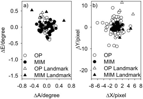
Fig. 4. Distribution of residuals in image (left panel) and angle
(right panel) coordinates for camera 1 (OP, open circles) and 2 (MIM, closed circles). Triangles denote landmark observations.
The rms angle residuals are in the range of 0.2◦or smaller, and the pixel residuals in the range of 3 (see Table 3 and Fig. 4). The pixel residuals for MIM are smaller and the angular residuals are larger than for OP because of coarser angular resolution per pixel. Given the short focal length of the cameras, and considering the fact that the angular diam-eter of the Sun and Moon is about 0.5◦, these residuals are within the expected measurement errors. Note, an angle er-ror of 0.2◦corresponds to 35 m displacement at 10 km alti-tude in the zenith above the MIM camera. The pixel residu-als are larger, mainly because of glare, but comparable to the accuracy of cloud feature observations. The landmarks are at very low elevation angles and at small distances, which could be a source of additional uncertainty, but the residuals are in the same range as for the other observations. Landmarks are time-independent and they show no systematic1A residu-als, which would arise from astronomical observations if the image time readings were systematically high or low.
To show the sensitivity to the distortion corrections (Eq. 3), we applied the model also without the corrections. In this case, the rms residuals become about 20 times larger. The radial corrections mainly reduce elevation residuals, while the affine transformation mainly impacts azimuth values. The importance of the radial transformation can also be seen from the factorb(Table 2) which amounts to about 3.5 %. The ex-ponential term becomes large for pixel radii larger than 1/c, of about 200 to 500.
U. Schumann et al.: Contrail camera observations 3603
Table 2. Model parameters.
No. Aˆ Bˆ Cˆ Dˆ Eˆ Fˆ
unit 1 1 1 1 1 1
1 0.9990 −0.2496×10⁻¹ −0.1893×10⁻² 0.2411×10⁻¹ 1.0000 −0.8236×10⁻²
2 0.9989 0.4294×10⁻¹ −0.7639×10⁻² −0.4460×10⁻¹ 0.9992 0.4115×10⁻³
3 1 0 0 0 1 0
4 0.9989 0.1955×10⁻¹ −0.3634×10⁻¹ −0.1413×10⁻¹ 0.1001×101 0.4599×10⁻¹
No. a b c X0 Y0 E0 A0
unit radians pixel−1 1 pixel−1 pixel pixel degree degree
1 0.7493×10⁻³ 0.3458×10⁻¹ 0.2291×10⁻² 1024 768 30.98 262.17
2 0.1747×10⁻² 0.4875×10⁻² 0.5566×10⁻² 638.68 483.49 90 0
3 0.3175×10⁻³ 0 0 1824 1368 27.74 120.82
4 0.2487×10⁻² 0.2466×10⁻¹ 0.8549×10⁻² 320 240 0.76 262.55
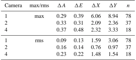
Table 3. Maximum and rms residuals in anglesA, E(in degree) and image coordinatesX, Y(in pixels) and number of observationsn.
Camera max/rms 1A 1E 1X 1Y n
1 max 0.29 0.39 6.06 8.94 78
2 0.33 0.31 2.09 2.36 37
4 0.37 0.48 2.32 3.33 18
1 rms 0.09 0.13 1.59 3.06 78
2 0.16 0.14 0.76 0.97 37
4 0.23 0.22 1.48 1.54 18
oscillations. This would be different, e.g., if a polynomial had been used. Tests have shown that the difference of pre-diction and measurement (in pixels) for the image distortion function, Eq. (3), does not exceed the typical measuring er-rors of a few pixels independent of the position angles in the image.
Finally, the observational data have to be sufficient for a stable computation of the affine transformation (Eq. 5). The parameters in this transformation become ill-defined if the image area covered by observations degrades to a line. For-tunately, for both cameras the covered areas have large ex-tensions in both coordinate directions. For modern cameras, we may expect nearly non-skewed and isotropic pixel orien-tations, so that Dˆ ≈ − ˆB, Eˆ ≈ ˆA. Here, Aˆ andEˆ differ by less than 0.01 % for both cameras. Small values ofBˆ andDˆ are expected if the camera mounting is precisely aligned hor-izontally. These relationships can also be used to assess the quality of the model input for a limited set of observations.
2.5 Transformations between observation angles and geographic coordinates
For relating geographic positions of an object to camera ob-servation angles, we use Cartesian coordinates (x, y, z), in m, with the horizontal planex–y tangential to a sphere, ap-proximating the Earth with mean radius R≈6371 km, at
longitudeλ=λC, latitudeφ=φC, and altitudez=zCof the camera C above mean sea level (a.s.l.). Here, x, y are the orthogonal horizontal geographic coordinates in eastern and northern directions andzis the vertical coordinate a.s.l. For small distancesλ−λCandφ−φC, the coordinatesx, y are related toλandφ, in degrees, approximately by
x−xC=(λ−λC)Rcos(φ)π/180◦, (23)
y−yC=(φ−φC)R π/180◦. (24)
For largeλ−λCandφ−φC, great circle computations (van de Kamp, 1967; Earle, 2005) are required instead.
In the computation of the elevation angleEand the pro-jected distance d on the ground between the object and the camera we account for the curvature of the Earth sur-face. Tests have shown that the curvature may be ignored for contrail altitude and wind speed determinations for al-titudes above 8 km and distances below 50 km. For larger distances and low elevation angles, however, the curvature must be considered. An object at altitudeH sinks below the horizon (E=0) at the horizontal distancea=
√
2RH+H2; e.g., a=35.7, 112.9, 357.1 km forH=0.1, 1, 10 km, re-spectively.
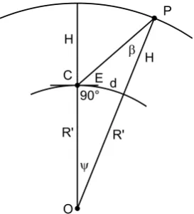
For an object P at altitudeH+zca.s.l. viewed from camera C at anglesA, E above Earth horizon with Earth origin in O and effective Earth radius R0=R+zC (see Fig. 5), the general triangle OCP is defined by two given side lengths OC and OP and one angle,ψ=d/Rorα=E+90◦. Hence, we find the distancedalong the Earth surface at sea level and the geographic coordinates(x, y)=g(A, E, H )from α=E+π/2, sin(β)=R
0sin (α)
R0+H , ψ=π−β−α, (25) d=ψ R, x=xC+dsin(A), y=yC+dcos(A). (26)
3604 U. Schumann et al.: Contrail camera observations
Fig. 5. Illustration of anglesE, β, ψ,distanced, altitudeH and effective Earth radiusR′=R+ ∆z Cfor an
object at position P and camera at C.
Fig. 6. A “4-contrail cross” formed by contrails C1, C2, C3, and C4 west of Oberpfaffenhofen and over Munich
between 08:39:08 and 08:55:15 UTC 3 November 2012. C5 is a short-lived contrail. Contrails and other clouds
appear white in front of the blue sky. The camera in OP is oriented westward covering elevations of about 0 to
60◦. The fisheye camera in MIM is oriented towards the zenith, with North, East, South, and West at the top,
right, bottom and left image boundaries, respectively. To compare cloud patterns in the photos from OP and
MIM, one has to rotate the MIM photos counterclockwise by about 90◦and to mirror along the West–East axis.
26
Fig. 5. Illustration of anglesE, β, ψ,distanced, altitudeH and effective Earth radiusR0=R+1zCfor an object at position P and
camera at C.
by d=
q
(x−xC)2+(y−yC)2, (27)
ψ= d
R, tan(γ )= H 2R0+H
1
tan(ψ/2), (28)
E=γ−ψ/2, A=tan−1[(x−xC)/(y−yC)]. (29) Similar relationships to computeA, E for given x, y, H are given in Garcia et al. (1997), but ours are simpler and al-low for explicit inversion to computex, yfor givenA, E, H.
3 A four-contrail-cross case study
3.1 Observations
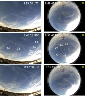
We observed four crossing contrails passing the view field of camera OP at about 08:42 UTC 3 November 2012 (see Fig. 6) (all the clock times refer to UTC). The air was clear with at least 100 km visibility. A westward wind was strong, with about 50 m s−1(e.g., according to ECMWF data) at the contrails’ altitudes, so that the contrails happened to move into the direction of Munich. Because of the cross pattern, the same set of contrails was clearly identified at MIM about 10 min later. The contrails are named C1, C2, C3 and C4, according to their clockwise appearance in the OP images. These observations will be used to determine the contrail al-titudes, tracking speeds, and widths. In addition, a short-lived contrail C5 was spotted. These observations also provide in-formation on the humidity.
The principle of this analysis can be understood from Fig. 7. The contrail (here C1) is observed by the two cameras at various times at various elevation angles between about 30 and 90◦, approaching OP from the west and passing MIM over a distance of about 50 km. The mean altitude and the mean speed of the contrail along thex axis are determined
by a fit to the observed elevation angle changes with time. Details are described in Sect. 3.2.
In addition to the contrails, some of the related aircraft were visible in the camera images. For contrails C1, C3, and C4, the contrail-causing aircraft could be detected in earlier images, either by spotting the aircraft themselves or their fresh trailing contrails. The times of first visibility and re-lated information are listed in Table 4. The aircraft causing contrail C2 was not visible, but the first detection of C2 west of OP at about 08:30 could be traced backwards with wind to identify the aircraft that caused this contrail in air traffic data a few minutes earlier.
The contrails were visible in the MIM images until about 09:09, i.e., for about 40 min. During this time, the contrails grew in width and got advected with the winds over a dis-tance of about 120 km. The contrails appeared to become optically thicker with time (measurements of the optical depth would require multispectral cameras, Seiz et al., 2007). Hence, all these contrails are classified to be persistent.
The same contrails were incidentally observed by a high resolution camera MAY from Munich (no. 3 in Table 1), 1.27 km north of MIM. This type 1 camera has a rather nar-row field of view with less distortion. Camera model 1 pro-vides a reasonable approximation for this camera even with-out corrections for radial or linear distortion. Since this cam-era is not in fixed position, we estimated orientation and scal-ing from 3 landmark and 3 Sun observations. The camera pointing accuracy is estimated to about 1◦, as supported by the observation of an aircraft with a shortly visible contrail, the position of which is given by ADSB data.
Finally a low-resolution webcam HOP (no. 4 in Table 1) of the Observatory Hohenpeissenberg (Deutscher Wetterdi-enst), 37.53 km southwest of OP, calibrated with a few Sun, Moon, star (Arcturus and Vega), and landmark observations, documents the scene in westward direction.
3.2 Contrail altitude and wind speed
U. Schumann et al.: Contrail camera observations 3605
Fig. 5. Illustration of angles
E, β, ψ,
distance
d
, altitude
H
and effective Earth radius
R
′=
R
+ ∆z
C
for an
object at position P and camera at C.
Fig. 6. A “4-contrail cross” formed by contrails C1, C2, C3, and C4 west of Oberpfaffenhofen and over Munich
between 08:39:08 and 08:55:15 UTC 3 November 2012. C5 is a short-lived contrail. Contrails and other clouds
appear white in front of the blue sky. The camera in OP is oriented westward covering elevations of about 0 to
60
◦. The fisheye camera in MIM is oriented towards the zenith, with North, East, South, and West at the top,
right, bottom and left image boundaries, respectively. To compare cloud patterns in the photos from OP and
MIM, one has to rotate the MIM photos counterclockwise by about 90
◦and to mirror along the West–East axis.
26
Fig. 6. A “four-contrail cross” formed by contrails C1, C2, C3, and C4 west of Oberpfaffenhofen and over Munich between 08:39:08 and
08:55:15 UTC 3 November 2012. C5 is a short-lived contrail. Contrails and other clouds appear white in front of the blue sky. The camera in OP is oriented westward covering elevations of about 0 to 60◦. The fisheye camera in MIM is oriented towards the zenith, with North, East, South, and West at the top, right, bottom and left image boundaries, respectively. To compare cloud patterns in the photos from OP and MIM, one has to rotate the MIM photos counterclockwise by about 90◦and to mirror along the West–East axis.
The contrail coordinates(x, y)are assumed to be close to straight lines
yc(t )=C(t )+s(t )xc(t ). (30)
The valuesCandsat various times are fitted so that the sum of(x−xc)2+(y−yc)2over all points along a contrail in a sin-gle image assumes its minimum. The plots in Fig. 8 show that the contrails are in fact very close to linear. This also shows that the camera model correctly removes the distortion of straight lines. For a moving line without marked features, one can determine the tracking speed only in the normal di-rection. Here, we follow the advection of the cross point be-tween the contrail lines and and the line connecting the two
3606 U. Schumann et al.: Contrail camera observations
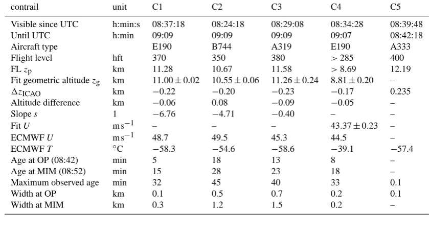
Table 4. Observed and computed contrail properties with FL pressure-altitude and observed geometric altitude a.s.l.
contrail unit C1 C2 C3 C4 C5
Visible since UTC h:min:s 08:37:18 08:24:18 08:29:08 08:34:28 08:39:48
Until UTC h:min 09:09 09:09 09:09 09:07 08:42:18
Aircraft type E190 B744 A319 E190 A333
Flight level hft 370 350 380 >285 400
FLzp km 11.28 10.67 11.58 >8.69 12.19
Fit geometric altitudezg km 11.00±0.02 10.55±0.06 11.26±0.24 8.81±0.20 –
1zICAO km −0.22 −0.20 −0.23 −0.17 0.235
Altitude difference km −0.06 0.08 −0.09 −0.05 –
Slopes 1 −6.76 −4.71 −0.40 – –
FitU m s−1 – – – 43.37±0.23 –
ECMWFU m s−1 48.7 49.5 45.3 44.5 –
ECMWFT ◦C −58.3 −54.6 −58.6 −39.1 −57.4
Age at OP (08:42) min 5 18 13 8 –
Age at MIM (08:52) min 15 28 23 18 –
Maximum observed age min 32 45 40 33 0.1
Width at OP km 0.1 0.5 0.7 0.2 0.1
Width at MIM km 0.3 1.2 1.5 0.2 –
Fig. 7. Viewing directions to contrail C1 from cameras OP and MIM at a sequence of times (08:39:08, 42:08,
42:38, 48:42, 51:43, 55:15 UTC, from left to right). The contrail altitude is the result of the fit described in
Sect. 3.2. The contrailxvalues are the positions where the contrail line cuts thexaxis through OP.
! " #
!
"
Fig. 8. Contrail horizontal coordinates (x, y; symbols) for contrails C1 to C4 at OP and MIM (times 08:39:08,
42:08, 42:38, 48:42, 51:43, 55:15 UTC) derived from the observations in images from cameras at OP and MIM.
The lines show the linear fits to the contrail positions as computed from the observed image pixles(X, Y)using
the camera models(A, E) =F(X, Y) and the geographic coordinates(x, y) =g(A, E, H)for fitted geometric
altitudesz=zC+Ha.s.l. Grey lines show lake positions for orientation.
Fig. 7. Viewing directions to contrail C1 from cameras OP and
MIM at a sequence of times (08:39:08, 42:08, 42:38, 48:42, 51:43, 55:15 UTC, from left to right). The contrail altitude is the result of the fit described in Sect. 3.2. The contrailxvalues are the positions where the contrail line cuts thexaxis through OP.
connection line between the cameras (C4 in our example), we need to identify contrail features (here the end points) which can be assumed to move with constant wind speed(U, V ).
Table 4 lists the results. The fit results are accurate of up to 230 m rms errors forz, and 0.23 m s−1 for advection or wind speed. This was found out by systematically repeating the analysis with random selections of subsets of the camera readingsX, Y. The rms error is largest for C3, which has an orientation not far different from the wind direction.
The contrail altitudes derived from the camera fits can be compared with the aircraft flight level information (see Table 4). Note that the camera observes the geometric al-titude. Aircraft flight levels (FL) are pressure altitudes zp in hft defined for static pressure in the International Civil Aviation Organization (ICAO) standard atmosphere (ICAO, 1964). In our case, with lower-than-average surface pres-sure and warmer atmosphere up to 8 km, the geometric (or geopotential) altitudezgis lower than the ICAO pressure alti-tudezp, according to ECMWF data, for this case (1zICAO=
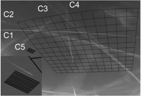
Fig. 9. Section of Fig. 6 (red color part), from OP at 08:40:28 UTC, with the 5 contrails C1 to C5, with two
grids of geographicx–ylines for orientation, a coarse one (1kmgrid spacing) atz= 11 kmaltitude a.s.l., and a fine one, rotated into flight direction of C5, with 100mgrid spacing, atz= 12 km. The insert in the lower left corner shows contrail C5 and the fine grid enlarged.
Fig. 10. Aircraft flight tracks (red lines) in horizontal coordinates(x, y)relative to the positions of the camera in Oberpfaffenhofen (OP, cross) as identified from aircraft waypoint data. Sightings of the aircraft (black circles
connected with black lines), based on pixel coordinates in the camera images and traffic data flight altitudes.
The single black circles for C2 and C4 denote the first contrail sighting. The blue lines (linear fits of observed
positions) locate the contrails C1 to C4 at times 08:42:38 and 08:51:43 UTC. Grey lines locate the lakes.
28
Fig. 8. Contrail horizontal coordinates (x, y; symbols) for contrails C1 to C4 at OP and MIM (times 08:39:08, 42:08, 42:38, 48:42, 51:43, 55:15 UTC) derived from the observations in images from cameras at OP and MIM. The lines show the linear fits to the contrail positions as computed from the observed image pixels(X, Y )using the camera models(A, E)=F (X, Y) and the geographic coordi-nates(x, y)=g(A, E, H )for fitted geometric altitudesz=zC+H
a.s.l. Grey lines show lake positions for orientation.
zg−zp= −200±30 m). Hence, the effective altitude differ-ence is zg−zp−1zICAO. With this correction, the altitude differences are within±100 m (see Table 4). The wind speed componentsU andV derived for case C4 at 8.7 km altitude
U. Schumann et al.: Contrail camera observations 3607
agree within 5 % with the ECMWF data (44.5 and 6 m s−1), see Fig. 13.
Errors of the order of 200 m my be acceptable when considering other sources of uncertainty: The lower part of a contrail sinks during the wake vortex phase by a range of the order of 50–300 m depending on aircraft and atmosphere parameters (e.g., Schumann et al., 2013). Differences may also result from uncertain pixel readings for thick contrails, horizontal variations in the wind speed (theUwind compo-nent seems to increase withy), and atmospheric wave mo-tions. However, the accuracy of the derived contrail altitudes is consistent with stereo camera cloud altitude results (Seiz et al., 2007).
For analysis of contrail widths, we use overlays of hor-izontalx–y grids into the image, as shown for example in Fig. 9. The geographic grid coordinatesx, y, zare specified for given contrail altitudes and given horizontal resolution. The view angles A, E and the image coordinatesX, Y are computed using Eqs. (1) and (29). The widths observed over OP and MIM, as listed in Table 4, are determined by match-ing the observed contrails with the grid, with about 100 m accuracy. The width of the short-lived contrail C5 is at the limit of resolution. For the others, the width accuracy is lim-ited mainly by the contrail shape and contrail edge contrast against clear sky. With time, the persistent contrails become wider. The width for C3 includes the sum of primary and secondary wake parts which can be visually distinguished in this case. Because of positive wind shear, the primary wake appears at the more westward edge.
3.3 Aircraft identification
For contrails C1, C3, and C5, the pixel coordinatesX, Y of the aircraft sightings were measured (typically with±2 pixel uncertainties). For C4, the first contrail appearance was lo-cated in the OP camera images. These data were converted into azimuth and elevation anglesA, Eusing the OP camera model, Eq. (1). With this information and an estimated alti-tudez, we use Eq. (26) to estimate the geographic horizontal coordinates(x, y, z, t )of the first contrail sightings.
From the German air traffic control agency (DFS, Deutsche Flugsicherung), we obtained the waypoint coor-dinates of all aircraft movements above about 7 km for this day over Germany. The data give the waypoint coordi-nates(x, y, z, t )in 1 min intervals. The DFS positions were compared with ADSB observations (available every 5 s). Presently, most aircraft in operation are equipped with ADSB transponders. Exceptions may occur in particular for small jets. The ADSB data cover all the flights for which contrails were identified in this case study, and give (within round-off or time interpolation errors) identical position values. For the following analysis, DFS data are used.
Plotting the coordinatesx, y, z, tof the first contrail sight-ing together with the coordinates of the aircraft waypoints, the aircraft flights could be identified without doubt even for
Fig. 9. Section of Fig. 6 (red color part), from OP at 08:40:28 UTC, with the 5 contrails C1 to C5, with two
grids of geographicx–ylines for orientation, a coarse one (1kmgrid spacing) atz= 11 kmaltitude a.s.l., and a fine one, rotated into flight direction of C5, with 100mgrid spacing, atz= 12 km. The insert in the lower left corner shows contrail C5 and the fine grid enlarged.
Fig. 10. Aircraft flight tracks (red lines) in horizontal coordinates(x, y)relative to the positions of the camera in Oberpfaffenhofen (OP, cross) as identified from aircraft waypoint data. Sightings of the aircraft (black circles
connected with black lines), based on pixel coordinates in the camera images and traffic data flight altitudes.
The single black circles for C2 and C4 denote the first contrail sighting. The blue lines (linear fits of observed
positions) locate the contrails C1 to C4 at times 08:42:38 and 08:51:43 UTC. Grey lines locate the lakes.
28
Fig. 9. Section of Fig. 6 (red color part), from OP at 08:40:28 UTC,
with the 5 contrails C1 to C5, with two grids of geographicx–y
lines for orientation, a coarse one (1 km grid spacing) atz=11 km altitude a.s.l., and a fine one, rotated into flight direction of C5, with 100 m grid spacing, atz=12 km. The insert in the lower left corner shows contrail C5 and the fine grid enlarged.
rough altitude estimates (about 10 km). With altitude from these data, the geographical coordinates of the contrail sight-ings were matched accurately. For example, Fig. 10 shows the positions of aircraft sightings together with the flight co-ordinates in anx–y plane. For given altitude, the horizon-tal aircraft positions as derived from the camera observations and from the waypoint data agree within 200 m, or better than 1 %, even at the most remote distances. This demonstrates nicely the accuracy of the camera model.
For C2, the aircraft was too far away (more than 70 km) to be visible in the photos. Here, Fig. 10 depicts the position of the first contrail sighting. An aircraft flying further west about 4 min before the first sighting caused contrail C2.
The position of the first appearance of C4 agrees accu-rately with the aircraft track (in horizontal position, time and altitude). The aircraft causing C4 was climbing while flying westward. The aircraft flight level listed below is that at the time of first contrail appearance.
An aircraft with the short contrail C5 (about 1 to 2 km length, i.e., less than 10 s maximum age) is visible in Fig. 6, at least in the full-resolution original images. From the ob-served coordinates and the waypoint data, the aircraft was clearly identified (see Fig. 10).
3.4 Synthetic contrail images
For given aircraft waypoint and wind information, the trajec-tories of the contrail waypoints can be computed using the Lagrangian advection part of CoCiP (Schumann, 2012) (see Fig. 11).
3608 U. Schumann et al.: Contrail camera observations
Fig. 7. Viewing directions to contrail C1 from cameras OP and MIM at a sequence of times (08:39:08, 42:08,
42:38, 48:42, 51:43, 55:15 UTC, from left to right). The contrail altitude is the result of the fit described in
Sect. 3.2. The contrailxvalues are the positions where the contrail line cuts thexaxis through OP.
!
" #
!
"
Fig. 8. Contrail horizontal coordinates (x, y; symbols) for contrails C1 to C4 at OP and MIM (times 08:39:08, 42:08, 42:38, 48:42, 51:43, 55:15 UTC) derived from the observations in images from cameras at OP and MIM.
The lines show the linear fits to the contrail positions as computed from the observed image pixles(X, Y)using the camera models(A, E) =F(X, Y) and the geographic coordinates(x, y) =g(A, E, H)for fitted geometric altitudesz=zC+Ha.s.l. Grey lines show lake positions for orientation.
27
Fig. 10. Aircraft flight tracks (red lines) in horizontal coordinates
(x, y)relative to the positions of the camera in Oberpfaffenhofen (OP, cross) as identified from aircraft waypoint data. Sightings of the aircraft (black circles connected with black lines), based on pixel coordinates in the camera images and traffic data flight alti-tudes. The single black circles for C2 and C4 denote the first con-trail sighting. The blue lines (linear fits of observed positions) locate the contrails C1 to C4 at times 08:42:38 and 08:51:43 UTC. Grey lines locate the lakes.
with 0.25◦ horizontal grid resolution are taken from hourly ECMWF forecasts starting 00:00 UTC 3 November 2012. With a second-order Runge–Kutta method, the wind defines the trajectory from the aircraft waypoints to new positions (x, y, z, t ) at time t > t0 of analysis. The NWP underesti-mates the real humidity at some flight levels (see Sect. 3.5). Therefore, instead of using humidity information from the NWP model as in other CoCiP applications, we simulate the contrails for constant supersaturation (about 10 %). We as-sume zero sedimentation because sedimentation depends on the particle sizes and these are strong functions of ambient supersaturation. Sedimentation has little effect on the young contrails. The persistent contrails spread with time as a func-tion of initial wake depth, shear, and turbulent diffusivities (Schumann, 2012; Schumann and Graf, 2013). The simu-lated contrails C1, C2, C3 and C4 over MIM are about 510, 370, 760, and 260 m wide, respectively.
For the computed geographic positions, we compute the angles(A, E)of the visual appearance of the waypoints for observers at the camera positions(xC, yC, zC)using Eq. (29). Then, the inverse camera model, Eq. (11), is used to com-pute the corresponding image points(X, Y ). The lines inter-connecting the individual image points are used to visualize the contrail appearance. The contrail lines are plotted as syn-thetic image together with the photo image of timet0 (see Fig. 11). For smooth plots of the contrail segments, several intermediate points (depending on distance from the camera) are created by linear interpolation along the flight segments
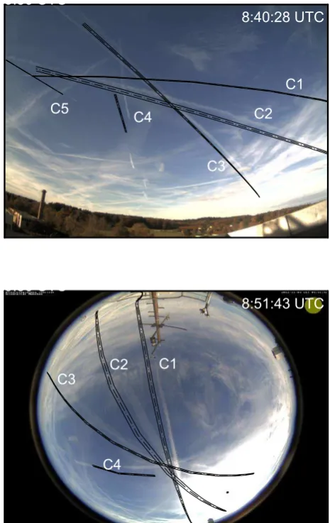
Fig. 11. Top panel: C1 to C5 contrail observations and computed positions (black lines) in the photo from OP
at 08:40:28 UTC. The contrail centers are indicated by dash-dotted lines, the lateral contrail boundaries by solid
lines. Note that for C1 and C5 most of the white contrail cloud in the photo is hidden by the computed position
lines. Bottom panel: same contrails (except C5) over MIM at 08:51:43 UTC.
29
Fig. 11. Top panel: C1 to C5 contrail observations and computed
positions (black lines) in the photo from OP at 08:40:28 UTC. The contrail centers are indicated by dash-dotted lines, the lateral con-trail boundaries by solid lines. Note that for C1 and C5 most of the white contrail cloud in the photo is hidden by the computed posi-tion lines. Bottom panel: same contrails (except C5) over MIM at 08:51:43 UTC.
in geographic space to provide about uniform angular reso-lution in the simulated images.
Contrail C4 was caused by a climbing aircraft but is vis-ible only along a short track. Perhaps this contrail formed in a rather thin layer of ice-supersaturation between 8.7 and 9 km pressure altitude. The contrails C1 to C4 persisted far after passing MIM. Contrail C5 is short-lived; we find no de-tectable trace of it in the MIM photos.
U. Schumann et al.: Contrail camera observations 3609
age mainly because of differences between NWP-derived and true wind speeds. Note, that 1 m s−1wind error for a con-trail age of 1000 s implies a position error of 1000 m, which corresponds to about 6◦ angular displacement for an over-head contrail at 10 km altitude. If contrail C1 were computed for a 15 s later time, its position would agree perfectly with the observation in the MIM photo. It seems that the true wind was slightly stronger than predicted by the NWP model, both inxandydirections.
Figure 11 also depicts the left and right boundaries of the contrails by plotting two lines at the same altitude as the con-trail center line, shifted laterally by the half widths in ge-ographic space. The computed and observed widths agree fairly well for C1, C4 and C5, but the observed contrails C2 and C3 are about a factor of two wider than simulated, possibly because of underestimate of small-scale shear in the NWP data. Contrail C4 experiences the weakest shear and may stays more narrow, therefore. Hence, such synthetic im-ages open a new approach to test and possibly improve con-trail modeling.
Synthetic contrails C1 to C4 were plotted also for the two other cameras. From HOP one of the four contrails (C2) was visible (at about 08:27) in reasonable agreement with syn-thetic images. From MAY, the contrail cross was observed and simulated while passing towards East (see Fig. 12). The picture supports the approximate validity of the synthetic contrail positions, and the persistence and increasing width of the contrails, besides many other interesting cirrus struc-tures.
3.5 Checks of humidity data and Schmidt–Appleman threshold
Contrail and cirrus properties are strongly sensitive to rela-tive humidity. Observations and numerical humidity predic-tions are difficult for many reasons. The formation of ice-supersaturation depends on vertical motion, temperature and cirrus ice microphysics (Tompkins et al., 2007). Layers of ice-supersaturation are often rather thin (Gierens et al., 2012) and hence difficult to resolve numerically.
Figure 13 shows wind, relative humidity over ice (RHi), and temperature vs. altitude as computed from ECMWF data. The model predicts ice-supersaturation between about 9.0 and 11.3 km pressure altitude, with a local minimum in RHi near 10.3 km altitude. For the NWP values of tempera-ture, humidity and pressure, and for aircraft burning kerosene with an overall propulsion efficiency of 0.3, the Schmidt– Appleman criterion (SAC) implies contrail formation for pressure altitudes zin the altitude range 9.5–16.5 km. The contrails C1 to C5, with the exception of C4, formed in this altitude range. C4 formed at about 0.7 km lower altitude. This indicates a possibly higher ambient humidity at this level than predicted by ECMWF.
At the altitudes of the observed persistent contrails, C1 to C4, the RHi must have been above 1. This is indicated by the
Fig. 12. Contrails C1 to C4 in the view of camera MAY, looking towards southeast, together with computed
contrails (as in Fig. 11), at 08:56:36 UTC.
! "
#
Fig. 13. Profiles of (a) horizontal wind speedsU,V in East and North directions, (b) relative humidity over ice RHi and maximum RHi (i.e. homogeneous nucleation limit), (c) temperature, from ECMWF data near OP (11◦E, 48◦N), vs. pressure altitude a.s.l. at 09:00 UTC. The symbols in (a) denote the wind speeds derived
from the camera observations for C4, the circles in (b) symbolize estimated RHi values for observed persistent or short contrails (grey or open) for the 5 contrails. In (c),TSAC,1is the Schmidt–Appleman criterion threshold temperature for contrail formation for the RHi obtained from ECMWF and an overall propulsion efficiency
η= 0.3;TSAC,2is the same for higherη(0.4) and RHi equal to RHimax.
30
Fig. 12. Contrails C1 to C4 in the view of camera MAY, looking
towards southeast, together with computed contrails (as in Fig. 11), at 08:56:36 UTC.
Fig. 12. Contrails C1 to C4 in the view of camera MAY, looking towards southeast, together with computed
contrails (as in Fig. 11), at 08:56:36 UTC.
! "
#
Fig. 13. Profiles of (a) horizontal wind speedsU,V in East and North directions, (b) relative humidity over
ice RHi and maximum RHi (i.e. homogeneous nucleation limit), (c) temperature, from ECMWF data near OP
(11◦E, 48◦N), vs. pressure altitude a.s.l. at 09:00 UTC. The symbols in (a) denote the wind speeds derived
from the camera observations for C4, the circles in (b) symbolize estimated RHi values for observed persistent
or short contrails (grey or open) for the 5 contrails. In (c),TSAC,1is the Schmidt–Appleman criterion threshold
temperature for contrail formation for the RHi obtained from ECMWF and an overall propulsion efficiency
η= 0.3;TSAC,2is the same for higherη(0.4) and RHi equal to RHimax.
30
Fig. 13. Profiles of (a) horizontal wind speedsU, V in East and North directions, (b) relative humidity over ice RHi and maximum RHi (i.e., homogeneous nucleation limit), (c) temperature, from ECMWF data near OP (11◦E, 48◦N), vs. pressure altitude a.s.l. at 09:00 UTC. The symbols in (a) denote the wind speeds derived from the camera observations for C4, the circles in (b) symbol-ize estimated RHi values for observed persistent or short contrails (grey or open) for the five contrails. In (c),TSAC,1is the Schmidt–
Appleman criterion threshold temperature for contrail formation for the RHi obtained from ECMWF and an overall propulsion effi-ciencyη=0.3;TSAC,2is the same for higherη(0.4) and RHi equal
to RHimax.
dots, though the true values of RHi remain uncertain. Any-way, the contrail observations imply supersaturation over a larger altitude range than predicted. The shortness of C4, formed by a climbing aircraft, indicates that the ECMWF analysis is correct in predicting a local RHi minimum at in-termediate altitudes between the levels of C4 and C2, i.e., at about 10 km. Here, RHi in fact might have dropped below one.
3610 U. Schumann et al.: Contrail camera observations
a function of ambient pressure, fuel properties (combustion heat and water emission index,Q=43.2 MJ kg−1, EI
H2O=
1.23), and overall propulsion efficiencyη(Schumann, 1996). ηmeasures the work performed by the aircraft engines by thrust and true air speed for given combustion heat and fuel flow per time unit. For cruising jet aircraft,ηis typically be-tween 0.3 and 0.38. Figure 13 showsTSAC,1, computed from ECMWF values for pressure and RHi and forη=0.3.
In this case, contrail C4 could not be explained. The am-bient temperature was about−39◦C, more than 7 K above the SAC temperature (−46.4◦C). The temperature accuracy of such NWP models is typically within 1 K (confirmed by comparison to other NWP output for this case). An increase ofηby 0.1 corresponds to an increase in RHi by 33 %; both cause 1.55 K higherTSAC. Hence, evenη=0.4 would not suffice to makeTSAClarger thanT. During climb, as in this case, η is usually smaller than at cruise because of lower aircraft speed. Hence, the ambient humidity must have been strongly ice-supersaturated. In clear air, humidity may reach or slightly exceed the homogeneous freezing limit (Koop et al., 2000), which equals liquid saturation nearT = −40◦C (about 1.45). Only with such high humidity, as indicated for C4 in Fig. 13, the atmosphere was just cold enough to let contrail C4 form as an exhaust contrail according to the Schmidt–Appleman criterion.
The short contrail C5 at 12.1 km indicates subsaturation at this pressure altitude. Hence, the NWP-predicted subsatura-tion atz >12 km (see Fig. 13) is confirmed by this contrail observation. From the results for C1–C4, the layer with ice-supersaturation reached over 8.6–11.8 km pressure altitude, nearly 40 % larger than predicted (9.0–11.3 km).
4 Conclusions
This paper describes methods for contrail tracking and anal-ysis of contrail properties from video camera observations, in particular contrail geometric altitudes, widths, and motion speeds. The methods are applied to a case study of contrail observations using two different kinds of wide-angle video cameras (whole-sky imager with fisheye lens or wide-angle cameras with smaller field of view), placed several kilome-ters apart.
Photogrammetric methods are described for the two cam-era types. The camcam-era models allow us to determine azimuth and elevation angles for given image coordinates and vice versa. The models account for linear and radial distortions. For the calibration we use mainly sightings of bright celes-tial objects together with some landmarks and aircraft with fresh contrail observations. An incomplete coverage of the field of view with such observations is overcome by exploit-ing reasonable symmetry assumptions in the camera mod-els. The accuracy of the models, demonstrated by the resid-uals between analyzed and observed coordinates and by the agreement of the observed positions of young contrails with
waypoint data, is within the range of the expected measuring errors.
The case study describes a “4-contrail cross” persisting for about 40 min, together with a short-lived one. Some of the contrail forming aircraft were visible and identified by com-parison to air traffic waypoint data. The waypoint informa-tion from DFS and from ADSB data was found to be in good agreement. The other contrails were related to aircraft flight tracks by means of contrail trajectories. From the comparison of observed positions with movement data, we found that the camera models and observations with two cameras allow de-termining the altitude and horizontal position of the contrails to an accuracy of better than 230 m, width to about 100 m, and the mean horizontal tracking speed to about 0.2 m s−1. In comparing altitudes, differences between ICAO standard at-mosphere pressure altitudes and geometric altitudes are sig-nificant.
The observed contrail evolution is compared with simu-lated contrails. Contrails are simusimu-lated with the contrail pre-diction model CoCiP, a Lagrangian model using air traffic movement data and numerical weather prediction (NWP) data as input. The results are projected on camera images. Here, the availability of the inverse camera model was essen-tial.
The presence of a contrail constrains the relative humid-ity being below or above the thresholds required for contrail formation (Schmidt–Appleman criterion) and contrail persis-tence (ice-supersaturation). The observations show spreading contrails, apparently with increasing optical depth, suggest-ing ice-supersaturated ambient air at contrail pressure alti-tudes (from 8.7 to 11.7 km). The ice-supersaturated layer is found considerably thicker than predicted by the NWP model used. In fact, to understand contrail C4 as being formed as an exhaust contrail, the aircraft must have flown in air with high relative humidity, close to liquid saturation at the time of contrail formation.
The model tends to underestimate the contrail widths, indi-cating underestimates in the initial contrail depth or ambient shear (from the NWP data) and turbulent mixing. With age, the horizontal contrail positions become increasingly sensi-tive to the assumed wind field. Although the camera derived wind data agree with ECMWF data within about 2 m s−1, such small differences cause notable shifts of aged contrails in the camera images.
U. Schumann et al.: Contrail camera observations 3611
combined with altitude information from other sources (e.g., ADSB data or ground-based lidar). The work described in this paper was initiated by observations of a special cirrus cloud which looked similar to contrails, but was not easily attributable to specific aircraft flights. The analysis of this special cirrus with the given photogrammetric methods and further observations is to be described in a future paper.
Acknowledgements. This paper is dedicated to the memory of
Her-mann Mannstein who died far too early in January 2013. He pio-neered cloud remote sensing at DLR for nearly three decades. His work on contrails is well known. Among others, he started the in-stallation and usage of ground-based cameras for contrail and cloud observations at DLR. On the morning of 3 November 2012, he noted many interesting cloud features and alerted his colleagues by send-ing photos from his private camera.
We thank Markus Rapp for hints to related studies of mesospheric objects, Ralf Meerkötter for general support, and Jürgen Oberst for providing experiences on meteor observations and helpful diploma theses on camera models by S. Elgner, T. Maue and S. Molau. We are grateful to F. Weber, DFS, for providing access to aircraft waypoint data, to Martin Schaefer for ADSB data, which are available from www.flightradar24.com, and were archived at DLR during the observation period, to Thomas Stark and Dieter Hausamann for landmark measurements at OP, and to Oliver Reitebuch for helpful comments on the manuscript. ECMWF data were provided within the project SPDERIMS.
The service charges for this open access publication have been covered by a Research Centre of the Helmholtz Association.
Edited by: M. Wendisch
References
Atlas, D. and Wang, Z.: Contrails of small and very
large optical depth, J. Atmos. Sci., 67, 3065–3073,
doi:10.1175/2010JAS3403.1, 2010.
Baumgarten, G., Fiedler, J., Fricke, K. H., Gerding, M., Hervig, M., Hoffmann, P., Müller, N., Pautet, P.-D., Rapp, M., Robert, C., Rusch, D., von Savigny, C., and Singer, W.: The noctilucent cloud (NLC) display during the ECOMA/MASS sounding rocket flights on 3 August 2007: morphology on global to local scales, Ann. Geophys., 27, 953–965, doi:10.5194/angeo-27-953-2009, 2009.
de Leege, A. M. P., Mulder, M., and van Paassen, M. M.: Novel method for wind estimation using automatic dependent surveillance-broadcast, J. Guid. Control Dynam., 35, 648–652, doi:10.2514/1.55833, 2012.
Duda, D. P., Palikonda, R., and Minnis, P.: Relating observations of contrail persistence to numerical weather analysis output, At-mos. Chem. Phys., 9, 1357–1364, doi:10.5194/acp-9-1357-2009, 2009.
Earle, M. A.: Vector solutions for great circle navigation, J. Naviga-tion, 58, 451–457, doi:10.1017/S0373463305003358, 2005. Feister, U. and Shields, J.: Cloud and radiance measurements
with the VIS/NIR Daylight Whole Sky Imager at
Linden-berg (Germany), Meteorol. Z., 14, 627–639, doi:10.1127/0941-2948/2005/0066, 2005.
Feister, U., Möller, H., Sattler, T., Shields, J., Görsdorf, U., and Güldner, J.: Comparison of macroscopic cloud data from ground-based measurements using VIS/NIR and IR instru-ments at Lindenberg, Germany, Atmos. Res., 96, 395–407, doi:10.1016/j.atmosres.2010.01.012, 2010.
Freudenthaler, V., Homburg, F., and Jäger, H.: Contrail observations by ground-based scanning lidar: cross-sectional growth, Geo-phys. Res. Lett., 22, 3501–3504, doi:10.1029/95GL03549, 1995. Garcia, F. J., Taylor, M. J., and Kelley, M. C.: Two-dimensional spectral analysis of mesospheric airglow image data, Appl. Op-tics, 36, 7374–7385, doi:10.1364/AO.36.007374, 1997. Gierens, K., Spichtinger, P., and Schumann, U.: Ice
supersatura-tion, in: Atmospheric Physics – Background – Methods – Trends, edited by: Schumann, U., doi:10.1007/978-3-642-30183-4_9, Springer, Berlin, Heidelberg, 2012.
Graf, K., Schumann, U., Mannstein, H., and Mayer, B.: Aviation induced diurnal North Atlantic cirrus cover cycle, Geophys. Res. Lett., 39, L16804, doi:10.1029/2012GL052590, 2012.
Heymsfield, A., Baumgardner, D., DeMott, P., Forster, P., Gierens, K., and Kärcher, B.: Contrail microphysics, B. Am. Me-teorol. Soc., 90, 465–472, doi:10.1175/2009BAMS2839.1, 2010. ICAO: Manual of the ICAO Standard Atmosphere, Tech. rep., ICAO Document No. 7488, 2nd Edn., International Civil Avi-ation OrganizAvi-ation, Montreal, 1964.
Immler, F., Treffeisen, R., Engelbart, D., Krüger, K., and Schrems, O.: Cirrus, contrails, and ice supersaturated regions in high pres-sure systems at northern mid latitudes, Atmos. Chem. Phys., 8, 1689–1699, doi:10.5194/acp-8-1689-2008, 2008.
Jackson, M. R. C., Sharma, V., Haissig, C. M., and Elgersma, M.: Airborne technology for distributed air traffic management, Eur. J. Control, 11, 464–477, doi:10.3166/ejc.11.464-477, 2005. Jeßberger, P., Voigt, C., Schumann, U., Sölch, I., Schlager, H.,
Kauf-mann, S., Petzold, A., Schäuble, D., and Gayet, J.-F.: Aircraft type influence on contrail properties, Atmos. Chem. Phys., 13, 11965–11984, doi:10.5194/acp-13-11965-2013, 2013.
Klaus, A., Bauer, J., Karner, K., Elbischger, P., Perko, R., and Bischof, H.: Camera calibration from a single night sky image, in: Proceedings of the 2004 IEEE Computer Society Conference on Computer Vision and Pattern Recognition, 27 June–2 July, CVPR 2004, Volume 1, Washington, D.C., 151–157, 2004. Koop, T., Luo, B., Tsias, A., and Peter, T.: Water activity as the
de-terminant for homogeneous ice nucleation in aqueous solutions, Nature, 406, 611–614, doi:10.1038/35020537, 2000.
LeMone, M. A., Schlatter, T. W., and Henson, R. T.: A strik-ing cloud over Boulder, Colorado: what is its altitude, and why does it matter?, B. Am. Meteorol. Soc., 94, 788–797, doi:10.1175/BAMS-D-12-00133.1, 2013.
Lewellen, D. C. and Lewellen, W. S.: Large-eddy simulations of the vortex-pair breakup in aircraft wakes, AIAA J., 34, 2337–2345, 1996.
Mannstein, H. and Schumann, U.: Aircraft induced contrail cirrus over Europe, Meteorol. Z., 14, 549–554, 2005.
Mannstein, H., Meyer, R., and Wendling, P.: Operational detection of contrails from NOAA-AVHRR data, Int. J. Remote Sens., 20, 1641–1660, 1999.
satel-3612 U. Schumann et al.: Contrail camera observations
lite imagery, Atmos. Meas. Tech., 3, 655–669, doi:10.5194/amt-3-655-2010, 2010.
Minnis, P., Bedka, S. T., Duda, D. P., Bedka, K. M., Chee, T., Ay-ers, J. K., Palikonda, R., Spangenberg, D. A., Khlopenkov, K. V., and Boeke, R.: Linear contrail and contrail cirrus properties de-termined from satellite data, Geophys. Res. Lett., 40, 3220–3226, doi:10.1002/grl.50569, 2013.
Oberst, J., Heinlein, D., Köhler, U., and Spurny, P.: The multiple meteorite fall of Neuschwanstein: circumstances of the event and meteorite search campaigns, Meteorit. Planet. Sci., 39, 1627– 1641, 2004.
Sassen, K.: Contrail-cirrus and their potential for regional climate change, B. Am. Meteorol. Soc., 78, 1885–1903, 1997.
Schumann, U.: On conditions for contrail formation from aircraft exhausts, Meteorol. Z., 5, 4–23, 1996.
Schumann, U.: A contrail cirrus prediction model, Geosci. Model Dev., 5, 543–580, doi:10.5194/gmd-5-543-2012, 2012.
Schumann, U. and Graf, K.: Aviation-induced cirrus and radiation changes at diurnal timescales, J. Geophys. Res., 118, 2404–2421, doi:10.1002/jgrd.50184, 2013.
Schumann, U., Mayer, B., Graf, K., and Mannstein, H.: A paramet-ric radiative forcing model for contrail cirrus, J. Appl. Meteorol. Clim., 51, 1391–1406, doi:10.1175/JAMC-D-11-0242.1, 2012. Schumann, U., Jeßberger, P., and Voigt, C.: Contrail ice particles
in aircraft wakes and their climatic importance, Geophys. Res. Lett., 40, 2867–2872 doi:10.1002/grl.50539, 2013.
Seiz, G., Shields, J., Feiste