Convolutional Neural Network for Paraphrase Identification
Wenpeng YinandHinrich Sch¨utze
Center for Information and Language Processing University of Munich, Germany
Abstract
We present a new deep learning architecture Bi-CNN-MI for paraphrase identification (PI). Based on the insight that PI requires compar-ing two sentenceson multiple levels of granu-larity, we learn multigranular sentence repre-sentations using convolutional neural network (CNN) and model interaction features at each level. These features are then the input to a logistic classifier for PI. All parameters of the model (for embeddings, convolution and clas-sification) are directly optimized for PI. To ad-dress the lack of training data, we pretrain the network in a novel way using a language mod-eling task. Results on the MSRP corpus sur-pass that of previous NN competitors.
1 Introduction
In this paper, we address the problem of paraphrase identification. It is usually formalized as a binary classification task: for two sentences(S1, S2),
deter-mine whether they roughly have the same meaning. Inspired by recent successes of deep neural networks (NNs) in fields like computer vision (Neverova et al., 2014), speech recognition (Deng et al., 2013) and natural language processing (Col-lobert and Weston, 2008), we adopt a deep learning approach to paraphrase identification in this paper.
The key observation that motivates our NN archi-tecture is that the identification of a paraphrase rela-tionship betweenS1 and S2 requires an analysisat
multiple levels of granularity.
(A1) “Detroit manufacturers have raised vehicle prices by ten percent.” – (A2) “GM, Ford and Chrysler have raised car prices by five percent.”
Example A1/A2 shows that paraphrase identifica-tion requires comparisonat the word level. A1 can-not be a paraphrase of A2 because the numbers “ten” and “five” are different.
(B1) “Mary gave birth to a son in 2000.” – (B2) “He is 14 years old and his mother is Mary.”
PI for B1/B2 can only succeed at the sentence level since B1/B2 express the same meaning using very different means.
Most work on paraphrase identification has fo-cused on only one level of granularity: either on low-level features (e.g., Madnani et al. (2012)) or on the sentence level (e.g., ARC-I, Hu et al. (2014)).
An exception is the RAE model (Socher et al., 2011). It computes representations on all levels of a parse tree: each node – including nodes corre-sponding to words, phrases and the entire sentence – is represented as a vector. RAE then computes a n1 ×n2 comparison matrix of the two trees
de-rived fromS1 andS2respectively, wheren1, n2are
the number of nodes and each comparison is the Eu-clidean distance between two vectors. This is then the basis for paraphrase classification.
RAE (Socher et al., 2011) is one of three prior NN architectures that we draw on to design our system. It embodies the key insight that paraphrase identi-fication involves analysis of information at multiple levels of granularity. However, relying on parsing has limitations for noisy text and for other applica-tions in which highly accurate parsers are not avail-able. We extend the basic idea of RAE by explor-ing stacked convolution layers which on one hand use sliding windows to split sentences into flexible phrases, furthermore, higher layers are able to
tract more abstract features of longer-range phrases by combining phrases in lower layers.
A representative way of doing this in deep learn-ing is the work by Kalchbrenner et al. (2014), the second prior NN architecture that we draw on. They use convolution to learn representations at multiple levels (Collobert and Weston, 2008). The motiva-tion for convolumotiva-tion is that natural language con-sists of long sequences in which many short sub-sequences contribute in a stable way to the struc-ture and meaning of the long sequence regardless of the position of the subsequence within the long sequence. Thus, it is advantageous to learn con-volutional filters that detect a particular feature re-gardless of position. Kalchbrenner et al. (2014)’s ar-chitecture extends this idea in two important ways. First, k-max pooling extracts the k top values from a sequence of convolutional filter applications and guarantees a fixed length output. Second, they stack several levels of convolutional filters, thus achieving multigranularity. We incorporate this architecture as the part that analyzes an individual sentence.
The third prior NN architecture we draw on is ARC proposed by Hu et al. (2014) who also attempt to exploit convolution for paraphrase identification. Their key insight is that we want to be able to di-rectly optimize the entire system for the task we are addressing,i.e., for paraphrase identification. Hu et al. (2014) do this by adopting a Siamese architec-ture: their NN consists of two shared-weight sen-tence analysis NNs that feed into a binary classi-fier that is directly trained on labeled sentence pairs. As we will show below, this is superior to separat-ing the two steps: first learnseparat-ing sentence represen-tations, then training binary classification for fixed, learned sentence representations as Bromley et al. (1993), Socher et al. (2011) and many others do.
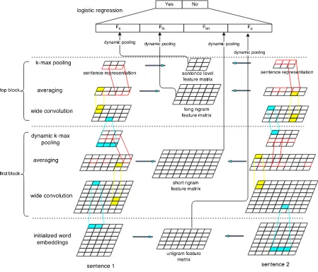
We can now give an overview of our NN architec-ture (Figure 1). We call it Bi-CNN-MI: “Bi-CNN” stands for double CNNs used in Siamese frame-work, “MI” for multigranular interaction features. Bi-CNN-MI has three parts: (i) the sentence anal-ysis network CNN-SM, (ii) the sentence interaction model CNN-IM and (iii) a logistic regression on top of the network that performs paraphrase identifica-tion. We now describe these three parts in detail.
(i) Following Kalchbrenner et al. (2014), we de-sign CNN-SM, a convolutional sentence analysis
NN that computes representations at four different levels: word, short ngram, long ngram and sentence. This multigranularity is important because para-phrase identification benefits from analyzing sen-tences at multiple levels.
(ii) Following Socher et al. (2011), CNN-IM, the interaction model, computes interaction features as s1×s2matrices, wheresiis the number of items of
a certain granularity inSi. In contrast to Socher et
al. (2011), CNN-IM computes these features at fixed levels and only for comparable units; e.g., we do not compare single words with entire sentences.
(iii) Following Hu et al. (2014), we integrate two copies of CNN-SM into a Siamese architecture that allows to optimize all parameters of the NN for para-phrase identification. In our case, these parameters include parameters for word embedding, for convo-lution filters, and for the classification of paraphrase candidate pairs. In contrast to Hu et al. (2014), the inputs to the final paraphrase candidate pair classifi-cation layer areinteraction feature matrices at mul-tiple levels– as opposed tosingle-level featuresthat do not directlycompare an element ofS1with a
po-tentially corresponding element ofS2.
There is one other problem we have to address to get good performance. Training sets for paraphrase identification are small in comparison with the high complexity of the task. Training a complex network like Bi-CNN-MI with a large number of parameters on a small training set is not promising due to sparse-ness and likely overfitting.
In order to make full use of the training data, we propose a new unsupervised training scheme CNN-LM (CNN Language Model) to pretrain the largest part of the model, the sentence analysis network CNN-SM. The key innovation is that we use a lan-guage modeling task in a setup similar to autoen-coding for pretraining (see below for details). This means that embedding and convolutional parameters can be pretrained on very large corpora since no hu-man labels are required for pretraining.
contribution of the paper independent of paraphrase identification.
Section 2 discusses related work. Sections 3 and 4 introduce the sentence model CNN-SM and the sentence interaction model CNN-IM. Section 5 de-scribes the training regime. The experiments are presented in Section 6. Section 7 concludes.
2 Related work
Bi-CNN-MI is closely related to NN models for sen-tence representations and for text matching.
A pioneering work using CNN to model sentences is (Collobert and Weston, 2008). They conducted convolutions on sliding windows of a sentence and finally use max pooling to form a sentence represen-tation. Kalchbrenner et al. (2014) introduce k-max pooling and stacking of several CNNs as discussed in Section 1.
Lu and Li (2013) developed a deep NN to match short texts, where interactions between components within the two objects were considered. These inter-actions were obtained via LDA (Blei et al., 2003). A two-dimensional interaction space is formed, then those local decisions will be sent to the correspond-ing neurons in upper layers to get rounds of fusion, finally logistic regression in the output layer pro-duces the final matching score. Drawbacks of this approach are that LDA parameters are not optimized for the paraphrase task and that the interactions are formed on the level of single words only.
Gao et al. (2014) model interestingnessbetween two documents with deep NNs. They map source-target document pairs to feature vectors in a latent space in such a way that the distance between the source document and its corresponding interesting target in that space is minimized. Interestingness is more like topic relevance, based mainly on the aggregate meaning of lots of keywords. Addition-ally, their model is a document-level model and is not multigranular.
Madnani et al. (2012) treated paraphrase relation-ship as a kind of mutual translation, hence combined eight kinds of machine translation metrics including BLEU (Papineni et al., 2002), NIST (Doddington, 2002), TER (Snover et al., 2006), TERp (Snover et al., 2009), METEOR (Denkowski and Lavie, 2010), SEPIA (Habash and Elkholy, 2008),
BAD-GER (Parker, 2008) and MAXSIM (Chan and Ng, 2008). These features are not multigranular; rather they are low-level only; high-level features – e.g., a representation of the entire sentence – are not con-sidered.
Bach et al. (2014) claimed that elementary dis-course units obtained by segmenting sentences play an important role in paraphrasing. Their conclu-sion also endorses Socher et al. (2011)’s and our work, for both take similarities between component phrases into account.
We discussed Socher et al. (2011)’s RAE and Hu et al. (2014)’s ARC-I in Section 1. In addition to similarity matrices there are two other important as-pects of (Socher et al., 2011). First, the similarity matrices are converted to a fixed size feature vector bydynamic pooling. We adopt this approach in Bi-CNN-MI; see Section 4.2 for details.
Second, (Socher et al., 2011) is partially based on parsing as is some other work on paraphrase iden-tification (e.g., Wan et al. (2006), Ji and Eisenstein (2013)). Parsing is a potentially powerful tool for identifying the important meaning units of a sen-tence, which can then be the basis for determining meaning equivalence. However, reliance on parsing makes these approaches less flexible. For example, there are no high-quality parsers available for some domains and some languages. Our approach is in principle applicable for any domain and language. It is also unclear how we would identify compara-ble units in the parse trees ofS1 andS2if the parse
trees have different height and the sentences differ-ent lengths. A key property of Bi-CNN-MI is that it is designed to produce units at fixed levels and only units at the same level are compared with each other.
3 Convolution sentence model CNN-SM Our network Bi-CNN-MI for paraphrase detection (Figure 1) consists of four parts. On the left and on the right there are two multilayer NNs with seven layers, from “initialized word embeddings: sentence 1/2” to “k-max pooling”. The weights of these two NNs are shared. This part of Bi-CNN-MI is based on (Kalchbrenner et al., 2014) and we refer to it as convolutional sentence model CNN-SM.
trices (unigram, short ngram, long ngram, sentence). CNN-IM feeds into a logistic classifier that performs paraphrase detection. See Sections 4 and 5 for these two parts of Bi-CNN-MI.
3.1 Wide convolution
We use Kalchbrenner et al. (2014)’s wide one-dimensional convolution. Denoting the number of tokens of Si as |Si|, we convolve weight matrix
M∈Rd×mover sentence representation matrixS∈
Rd×|Si| and generate a matrixC ∈ Rd×(|Si|+m−1)
each column of which is the representation of an m-gram. dis the dimension of word (and also ngram) embeddings.mis filter width.
Our motivation for using convolution is that af-ter training, a convolutional filaf-ter corresponds to a feature detector that learns to recognize a class of m-grams that is useful for paraphrase detection.
3.2 Averaging
After convolution, to build simple relations across rows, each odd row and the row behind im-mediately are averaged, generating matrix A ∈
Rd2×(|Si|+m−1). Namely:
A= (Codd+Ceven)/2 (1)
whereCodd,Ceven denote the odd and even rows of
C, respectively. Finally, this convolution layer will output matrixBwhosejth column is defined thus:
B:,j = tanh(A:,j+bT) 0≤j <(|Si|+m−1)
(2) bis a bias vector with dimensiond/2, same for each column.
3.3 Dynamic k-max pooling
We use Kalchbrenner et al. (2014)’s dynamic k-max poolingto extract features for variable-length sentences. It extractskdy top values from each
di-mension after the first layer of averaging andktop=
4top values after the top layer of averaging. We set
kdy= max(ktop,|Si|/2 + 1) (3)
Thus,kdydepends on the length ofSi.
The sequence of layers in (Kalchbrenner et al., 2014) is convolution, folding, k-max pooling,tanh. We experimented with this sequence and found that
after k-max pooling many tanh units had an input close to 1, in the nondynamic range of the function (since the input is the addition of several values). This makes learning difficult. We therefore changed the sequence to convolution, averaging,tanh, k-max pooling. This makes it less likely thattanhunits will be saturated.
We have described convolution, averaging and k-max pooling. We can stack several blocks of these three layers to form deep architectures, as the two blocks (marked “first block” and “top block”) in Fig-ure 1.
4 Convolution interaction model CNN-IM After the introduction in the previous section of the CNN-SM part of our architecture for processing an individual sentence, we now turn to the CNN-IM in-teraction model that computes the four feature ma-trices in Figure 1 to assess theinteractions between the two sentences.
4.1 Feature matrices
One key innovation of our approach is multigranu-larity: we compute similarity between the two para-phrase candidates on multiple levels. Specifically, we compute similarity at four levels in this paper: unigram, short ngram, long ngram and sentence. We use notationl∈ {u,sn,ln,s}to refer to the four lev-els, and use Si,l to denote the matrix representing
sentenceSi at levell. For levell, we compute
fea-ture matricesFˆlas follows:
ˆ
Fijl = exp(−||S
1,l
:,i −S2:,j,l||2
2β ) (4)
where||S1:,i,l −S2:,j,l||2 is the Euclidean distance
be-tween the representations of the ith item of S1 and
thejth item ofS2 on levell. We setβ = 2(cf. Wu
et al. (2013)).
We do not use cosine because the magnitude of the activations of hidden units is important, not just the overall direction; e.g., if S1:,i,l and S2:,j,l point in the same direction, but activations are much larger inS2:,j,l, then the two vectors are very dissimilar.
The lowest level feature matrix (l =u) is the un-igram similarity matrixFˆu. It has size|S1| × |S2|.
The feature entryFˆuij is the similarity between the
word is represented by a d-dimensional word em-bedding (d= 100in our experiments).
The next level feature matrix is the short ngram similarity matrixFˆsn. It has size(|S1|+msn−1)×
(|S2|+msn−1)wheremsn= 3is the filter width in
this convolution layer and|Si|+msn−1is the
num-ber of short ngrams inSi. The feature entryFˆsnij is
the similarity between twod/2-dimensional vectors representing two short ngrams fromS1andS2.
We use multiple feature maps to improve the sys-tem performance. Different feature maps are ex-pected to extract different kinds of sentence features, and can be implemented in the same convolution layer in parallel. Specifically, we use fsn = 6
fea-ture maps on this level following Kalchbrenner et al. (2014). Thus, we actually compute six feature ma-trices Fˆsn,i (i = 1,· · ·, fsn), one for each pair of
feature maps that share convolution weights while derived fromS1 andS2respectively. (Figure 1 only
shows one of those six matrices.)
The next level feature matrix is the long ngram similarity matrixFˆln. It has size(kdy,1+mln−1)×
(kdy,2 +mln −1) where kdy,i (Equation 3) is the
k value in dynamic k-max pooling for sentence i, kdy,i +mln −1 is the number of long ngrams in
Si and mln = 5is the filter width in this
convolu-tion layer. The feature entry Fˆlnij is the similarity
between two d/4-dimensional vectors representing two long ngrams fromS1andS2.
We use fln = 14feature maps on this level
fol-lowing Kalchbrenner et al. (2014). Thus, we com-pute 14 feature matricesFˆln,i (i = 1,· · ·, fln), in a
way analogous to thefsn= 6feature mapsFˆsn,i.
The last feature matrix is the sentence similarity matrix Fˆs. It has sizektop ×ktop wherektop = 4
is the parameter in k-max pooling at the last max pooling layer. The feature entryFˆsijis the similarity
between twod/4-dimensional vectors computed by max pooling fromS1andS2.
Forl=s, there are alsofln= 14feature matrices
ˆ
Fs,i (i = 1,· · ·, fln), analogous to the fln = 14
feature matricesFˆln,i.
A general design principle of the architecture is that we compute each interaction feature matrix be-tween two feature maps that share the same convo-lution weights. Two feature maps learned with the same filter will contain the same kinds of features derived from the input.
4.2 Dynamic pooling of feature matrices
As sentence lengths vary, feature matrices Fˆl have
different sizes, which makes it impossible to use them directly as input of the last layer.
That means we need to mapFˆl ∈ Rr×c into a
matrix Fl of fixed size r0 ×c0 (l ∈ {u,sn,ln,s};
r0, c0 are parameters and are the same for all
sen-tence pairs whiler, cdepend on|S1|and|S2|).
Dy-namic pooling dividesFˆlintor0×c0nonoverlapping
(dynamic) pools and copies the maximum value in each dynamic pool to Fl. Our method is similar to
(Socher et al., 2011), but preserves locality better. ˆ
Fl can be split into equal regions only ifr (resp.
c) is divisible byr0(resp.c0). Otherwise, forr > r0
and if rmodr0 = b, the dynamic pools in the first
r0−bsplits each haver r0
rows while the remaining bsplits each haverr0
+ 1rows. In Figure 2, ar×
c = 4×5matrix (left) is split intor0×c0 = 3×3
dynamic pools (middle): each row is split into [1, 1, 2] and each column is split into [1, 2, 2].
Ifr < r0, we first repeat all rows until no fewer
than r0 rows remain. Then first r0 rows are kept
and split into r0 dynamic pools. The same
princi-ple applies to the partitioning of columns. In Fig-ure 2 (right), the areas with dashed lines and dotted lines are repeated parts for rows and columns, re-spectively; each cell is its own dynamic pool.
5 Training
5.1 Supervised training
Dynamic pooling gives us fixed size interaction fea-ture matrices for sentence, ngram and unigram lev-els. As shown in Figure 1, the concatenation of these features (Fs,Fln,FsnandFu) is the input to a
logis-tic regression layer for paraphrase classification. We have now described all three parts of Bi-CNN-MI: CNN-SM, CNN-IM and logistic regression.
Bi-CNN-MI with all its parameters – includ-ing word embeddinclud-ings and convolution weights – is trained on MSRP. We initialize embeddings with those provided by Turian et al. (2010)1 (based on
Collobert and Weston (2008)). For layer sn, we have fsn = 6feature maps and set filter widthmsn = 3.
For layer ln, we havefln = 14feature maps and set
Figure 2: Partition methods in dynamic pooling. Original matrix with size4×5is mapped into matrix with size3×3
and matrix with size6×7, respectively. Each dynamic pool is distinguished by a border of empty white space around it.
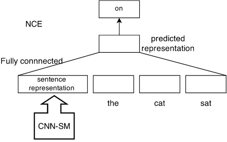
Figure 3: Unsupervised architecture: CNN-LM
sizes are10×10,10×10,6×6,2×2for unigram, short ngram, long ngram and sentence, respectively. For training, we employ mini-batch of size 70, L2
regularization with weight 5×10⁻⁴ and Adagrad
(Duchi et al., 2011).
5.2 Unsupervised pretraining
One of the key contributions of this paper is the ar-chitecture CNN-LM shown in Figure 3. CNN-LM is used to pretrain the convolutional filters on unla-beled data. This addresses sparseness and limited training data for paraphrase identification.
The convolution sentence model CNN-SM (Sec-tion 3) is part of CNN-LM (“CNN-SM” in Figure 3). The input to CNN-SM is the entire sentence (“the cat sat on the mat”); its output (“sentence represen-tation” in the leftmost rectangle in Figure 3 and the
two grids labeled “sentence representation” in the top layer of the top block in Figure 1) is concate-nated with a history consisting of the embeddings of theh= 3preceding words (“the”, “cat”, “sat”) as the input of a fully connected layer to generate a pre-dicted representation for the next word (“on”). We employ noise-contrastive estimation (NCE) (Mnih and Teh, 2012; Mnih and Kavukcuoglu, 2013) to compute the cost: the model learns to discriminate between true next words and noise words. NCE al-lows us to fit unnormalized models making the train-ing time effectively independent of the vocabulary size.
In experiments, CNN-LM is trained on unlabeled MSRP data and an additional 100,000 sentences from English Gigaword (Graff et al., 2003). In prin-ciple, sentences from any source, not just English Gigaword, can be used to train this model. In NCE, 20 noise words are sampled for each true example.
So training has two parts: unsupervised, CNN-LM (Figure 3) and supervised, Bi-CNN-MI (Fig-ure 1). In the first phase, the unsupervised training phase, we adopt a language modeling approach be-cause it does not require human labels and can use large corpora to pretrain word embeddings and con-volution weights. The goal is to learn sentence fea-tures that are unbiased and reflect useful attributes of the input sentence. More importantly, pretraining is useful to relieve overfitting, which is a severe prob-lem when building deep NNs on small corpora like MSRP (cf. Hu et al. (2014)).
[image:7.612.72.302.262.406.2]weights are tuned for optimal performance on PI. In CNN-LM, we have combined several architec-tural elements to pretrain a high-quality sentence analysis NN despite the lack of training data. (i) Similar to PV-DM (Le and Mikolov, 2014), we in-tegrate global context (CNN-SM) and local context (the history of size h) into one model – although our global context consists only of a sentence, not of a paragraph or document. (ii) Similar to work on autoencoding (Vincent et al., 2010), the output that is to be predicted is part of the input. Au-toencoding is a successful approach to learning rep-resentations and we adapt it here to pretrain good sentence representations. (iii) A second successful approach to learning embeddings is neural network language modeling (Bengio et al., 2003; Mikolov, 2012). Again, we adopt this by including in CNN-LM an ngram language modeling part to predict the next word. The great advantage of this type of em-bedding learning is that no labels are needed. (iv) LM only adds one hidden layer over CNN-SM. It keeps simple architecture like PV-DM (Le and Mikolov, 2014), CBOW (Mikolov et al., 2013) and LBL (Mnih and Teh, 2012), enabling the CNN-SM as main training target.
In summary, the key contribution of CNN-LM is that we pretrain convolutional filters. Architectural elements from the literature are combined to support effective pretraining of convolutional filters.
6 Experiments
6.1 Data set and evaluation metrics
We use the Microsoft Research Paraphrase Corpus (MSRP) (Dolan et al., 2004; Das and Smith, 2009). The training set contains 2753 true and 1323 false paraphrase pairs; the test set contains 1147 and 578 pairs, respectively. For each triple (label,S1,S2) in
the training set we also add (label,S2,S1) to make
best use of the training data; these additions are nonredundant because the interaction feature matri-ces (Section 4.1) are asymmetric. Systems are eval-uated by accuracy andF1.
6.2 Paraphrase detection systems
Since we want to show that Bi-CNN-MI performs better than previous NN work, we compare with three NN approaches: NLM, ARC and RAE
(Ta-ble 1).2 We also include the majority baseline
(“baseline”) and MT (Madnani et al., 2012). RAE
(Socher et al., 2011) andMTwere discussed in Sec-tions 1 and 2. We now briefly describe the other prior work.
Blacoe and Lapata (2012) compute the vector representation of a sentence from the neural lan-guage model (NLM) embeddings (computed based on (Collobert and Weston, 2008)) of the words of the sentence as the sum of the word embeddings (NLM+), as the element-wise multiplication of the word embeddings (NLM), or by means of the recursive autoencoder (NLM RAE, Socher et al. (2011)). The representations of the two paraphrase candidates are then concatenated as input to an SVM classifier. See Blacoe and Lapata (2012) for details.
The ARC model (Hu et al., 2014) is a convolu-tional architecture similar to (Collobert and Weston, 2008). ARC-I is a Siamese architecture in which two shared-weight convolutional sentence models are trained on the binary paraphrase detection task. Hu et al. (2014) find that ARC-I is suboptimal in that it defers the interaction between S1 and S2 to
the very end of processing: only after the vectors representingS1andS2have been computed does an
interaction occur. To remedy this problem, they pro-pose ARC-II in which the Siamese architecture is replaced by a multilayer NN that processes a single representation produced by interleavingS1andS2.
We also evaluateBi-CNN-MI–, an NN identical to Bi-CNN-MI, except that it is not pretrained in un-supervised training.
6.3 Results
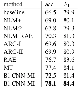
Table 1 shows that Bi-CNN-MI outperforms all other systems. The comparison with Bi-CNN-MI– indicates that this is partly due to one major in-novation we introduced: unsupervised pretraining. Bi-CNN-MI–, the model without unsupervised pre-training, performs badly. Thus, unsupervised train-ing is helpful to pretrain parameters in paraphrase
2A reviewer suggests an additional experiment to directly
method acc F1
baseline 66.5 79.9
NLM+ 69.0 80.1
NLM 67.8 79.3
NLM RAE 70.3 81.3
ARC-I 69.6 80.3
ARC-II 69.9 80.9
RAE 76.7 83.6
MT 77.4 84.1
Bi-CNN-MI– 72.5 81.4
[image:9.612.117.250.59.207.2]Bi-CNN-MI 78.1 84.4
Table 1: Performance of different systems on MSRP
features used acc F1
1 no features 66.5 79.9
2 + u: unigram 68.4 79.7
3 + sn: short ngram 75.3 82.8
4 + ln: long ngram 76.2 83.1
5 + s: sentence 73.4 82.3
6 – u: unigram 77.8 84.3
7 – sn: short ngram 76.3 83.5
8 – ln: long ngram 75.6 83.2
9 – s: sentence 77.6 84.2
[image:9.612.94.271.246.398.2]10 all features 78.1 84.4
Table 2: Analysis of impact of the four feature classes. Line 1: majority baseline. Line 10: Bi-CNN-MI result from Table 1. Lines 2–5: Bi-CNN-MI when only one feature class is used. Line 6–9: ablation experiment: on each line one feature class is removed.
detection, especially when the training set is small. RAE also uses pretraining, but not as effectively as Bi-CNN-MI as Table 1 indicates. Hu et al. (2014) also suggest that training complex NNs only with supervised training runs the risk of overfitting on the small MSRP corpus.
Table 2 looks at the relative importance of the four feature matrices shown in Figure 1. (The unsuper-vised part of the training regime is not changed for this experiment.) The results indicate that levels sn and ln are most informative: F1 scores are highest
if only these two levels are used (lines 3&4: 82.8, 83.1) and performance drops most when they are re-moved (lines 7&8: 83.5, 83.2).
Unigrams contribute little to overall performance (lines 2&6), probably because the paraphrases in the
corpus typically do not involve individual words (re-placing one word by its synonym); rather, the para-phrase relationship involves larger context, which can only be judged by the higher-level features.
Just using the sentence matrix by itself performs well (line 5), but less well than using only levels sn or ln (lines 3&4). Most prior NN work on PI has taken the sentence-level approach. Our results indi-cate that combining this with the more fine-grained comparison on the ngram-level is superior.
Removing the sentence matrix results in a small drop in performance (line 9). The reason is that sen-tence representations are computed by k-max pool-ing from level ln. Thus, we can roughly view the sentence-level feature matrixFsas a subset ofFln.
Adding (Madnani et al., 2012)’s MT metrics as input to the Bi-CNN-MI logistic regression further improves performance: accuracy of 78.4 andF1 of
84.6.
7 Conclusion and future work
We presented the deep learning architecture Bi-CNN-MI for paraphrase identification (PI). Based on the insight that PI requires comparing two sen-tences on multiple levels of granularity, we learn multigranular sentence representations using convo-lution and compute interaction feature matrices at each level. These matrices are then the input to a logistic classifier for PI. All parameters of the model (for embeddings, convolution and classification) are directly optimized for PI. To address the lack of training data, we pretrain the network in a novel way for a language modeling task. Results on MSRP are state of the art.
In the future, we plan to apply Bi-CNN-MI to sen-tence matching, question answering and other tasks. Acknowledgments
References
Ngo Xuan Bach, Nguyen Le Minh, and Akira Shi-mazu. 2014. Exploiting discourse information to identify paraphrases. Expert Systems with Applica-tions, 41(6):2832–2841.
Yoshua Bengio, R´ejean Ducharme, Pascal Vincent, and Christian Jauvin. 2003. A neural probabilistic lan-guage model. Journal of Machine Learning Research, 3:1137–1155.
William Blacoe and Mirella Lapata. 2012. A compari-son of vector-based representations for semantic com-position. InProceedings of the 2012 Joint Conference on Empirical Methods in Natural Language Process-ing and Computational Natural Language LearnProcess-ing, pages 546–556.
David M Blei, Andrew Y Ng, and Michael I Jordan. 2003. Latent dirichlet allocation. the Journal of ma-chine Learning research, 3:993–1022.
Jane Bromley, James W Bentz, L´eon Bottou, Isabelle Guyon, Yann LeCun, Cliff Moore, Eduard S¨ackinger, and Roopak Shah. 1993. Signature verification using a “siamese” time delay neural network. International Journal of Pattern Recognition and Artificial Intelli-gence, 7(04):669–688.
Yee Seng Chan and Hwee Tou Ng. 2008. Maxsim: A maximum similarity metric for machine translation evaluation. InACL, pages 55–62.
Ronan Collobert and Jason Weston. 2008. A unified ar-chitecture for natural language processing: Deep neu-ral networks with multitask learning. In Proceedings of the 25th international conference on Machine learn-ing, pages 160–167.
Dipanjan Das and Noah A Smith. 2009. Paraphrase iden-tification as probabilistic quasi-synchronous recogni-tion. In Proceedings of the Joint Conference of the 47th Annual Meeting of the ACL and the 4th Inter-national Joint Conference on Natural Language Pro-cessing of the AFNLP: Volume 1-Volume 1, pages 468– 476.
Li Deng, Geoffrey Hinton, and Brian Kingsbury. 2013. New types of deep neural network learning for speech recognition and related applications: An overview. In Acoustics, Speech and Signal Processing (ICASSP), 2013 IEEE International Conference on, pages 8599– 8603.
Michael Denkowski and Alon Lavie. 2010. Extending the meteor machine translation evaluation metric to the phrase level. InHuman Language Technologies: The 2010 Annual Conference of the North American Chap-ter of the Association for Computational Linguistics, pages 250–253.
George Doddington. 2002. Automatic evaluation of ma-chine translation quality using n-gram co-occurrence
statistics. In Proceedings of the second interna-tional conference on Human Language Technology Research, pages 138–145.
Bill Dolan, Chris Quirk, and Chris Brockett. 2004. Un-supervised construction of large paraphrase corpora: Exploiting massively parallel news sources. In Pro-ceedings of the 20th international conference on Com-putational Linguistics, page 350.
John Duchi, Elad Hazan, and Yoram Singer. 2011. Adaptive subgradient methods for online learning and stochastic optimization. The Journal of Machine Learning Research, 12:2121–2159.
Jianfeng Gao, Patrick Pantel, Michael Gamon, Xiaodong He, Li Deng, and Yelong Shen. 2014. Modeling inter-estingness with deep neural networks. InProceedings of the 2013 Conference on Empirical Methods in Nat-ural Language Processing.
David Graff, Junbo Kong, Ke Chen, and Kazuaki Maeda. 2003. English gigaword.Linguistic Data Consortium, Philadelphia.
Nizar Habash and Ahmed Elkholy. 2008. Sepia: sur-face span extension to syntactic dependency precision-based mt evaluation. InProceedings of the NIST met-rics for machine translation workshop at the associ-ation for machine translassoci-ation in the Americas confer-ence, AMTA-2008. Waikiki, HI.
Baotian Hu, Zhengdong Lu, Hang Li, and Qingcai Chen. 2014. Convolutional neural network architectures for matching natural language sentences. InAdvances in Neural Information Processing Systems.
Yangfeng Ji and Jacob Eisenstein. 2013. Discriminative improvements to distributional sentence similarity. In Proceedings of the Conference on Empirical Methods in Natural Language Processing.
Nal Kalchbrenner, Edward Grefenstette, and Phil Blun-som. 2014. A convolutional neural network for mod-elling sentences. InProceedings of the 52nd Annual Meeting of the Association for Computational Linguis-tics.
Quoc V Le and Tomas Mikolov. 2014. Distributed rep-resentations of sentences and documents. In Proceed-ings of the 31th international conference on Machine learning.
Zhengdong Lu and Hang Li. 2013. A deep architecture for matching short texts. InAdvances in Neural Infor-mation Processing Systems, pages 1367–1375. Nitin Madnani, Joel Tetreault, and Martin Chodorow.
2012. Re-examining machine translation metrics for paraphrase identification. InProceedings of the 2012 NAACL-HLT, pages 182–190.
Tom´aˇs Mikolov. 2012. Statistical language models based on neural networks. Ph.D. thesis, Ph. D. the-sis, Brno University of Technology.
Andriy Mnih and Koray Kavukcuoglu. 2013. Learning word embeddings efficiently with noise-contrastive es-timation. InAdvances in Neural Information Process-ing Systems, pages 2265–2273.
Andriy Mnih and Yee Whye Teh. 2012. A fast and sim-ple algorithm for training neural probabilistic language models. InProceedings of the 29th International Con-ference on Machine Learning, pages 1751–1758. N Neverova, C Wolf, GW Taylor, and F Nebout. 2014.
Multi-scale deep learning for gesture detection and lo-calization. InEuropean Conference on Computer Vi-sion (ECCV) 2014 ChaLearn Workshop. Zurich. Kishore Papineni, Salim Roukos, Todd Ward, and
Wei-Jing Zhu. 2002. Bleu: a method for automatic evalua-tion of machine translaevalua-tion. InProceedings of the 40th ACL, pages 311–318.
Steven Parker. 2008. Badger: A new machine translation metric.Metrics for Machine Translation Challenge. Matthew Snover, Bonnie Dorr, Richard Schwartz,
Lin-nea Micciulla, and John Makhoul. 2006. A study of translation edit rate with targeted human annotation. InProceedings of association for machine translation in the Americas, pages 223–231.
Matthew G Snover, Nitin Madnani, Bonnie Dorr, and Richard Schwartz. 2009. Ter-plus: paraphrase, se-mantic, and alignment enhancements to translation edit rate. Machine Translation, 23(2-3):117–127. Richard Socher, Eric H Huang, Jeffrey Pennin,
Christo-pher D Manning, and Andrew Y Ng. 2011. Dynamic pooling and unfolding recursive autoencoders for para-phrase detection. In Advances in Neural Information Processing Systems, pages 801–809.
Joseph Turian, Lev Ratinov, and Yoshua Bengio. 2010. Word representations: a simple and general method for semi-supervised learning. InProceedings of the 48th Annual Meeting of the Association for Computational Linguistics, pages 384–394.
Pascal Vincent, Hugo Larochelle, Isabelle Lajoie, Yoshua Bengio, and Pierre-Antoine Manzagol. 2010. Stacked denoising autoencoders: Learning useful representa-tions in a deep network with a local denoising cri-terion. The Journal of Machine Learning Research, 11:3371–3408.
Stephen Wan, Mark Dras, Robert Dale, and C´ecile Paris. 2006. Using dependency-based features to take the “para-farce” out of paraphrase. InProceedings of the Australasian Language Technology Workshop, volume 2006.
Pengcheng Wu, Steven CH Hoi, Hao Xia, Peilin Zhao, Dayong Wang, and Chunyan Miao. 2013. Online