On Evaluating the Generalization of LSTM Models in Formal Languages
Mirac Suzgun Yonatan Belinkov Stuart M. Shieber
John A. Paulson School of Engineering and Applied Sciences Harvard University
Cambridge, MA 02138, USA
{msuzgun@college,belinkov@seas,shieber@seas}.harvard.edu
Abstract
Recurrent Neural Networks (RNNs) are the-oretically Turing-complete and established themselves as a dominant model for language processing. Yet, there still remains an uncer-tainty regarding their language learning capa-bilities. In this paper, we empirically evalu-ate the inductive learning capabilities of Long Short-Term Memory networks, a popular ex-tension of simple RNNs, to learn simple for-mal languages, in particular anbn, anbncn, andanbncndn. We investigate the influence of various aspects of learning, such as train-ing data regimes and model capacity, on the generalization to unobserved samples. We find striking differences in model performances un-der different training settings and highlight the need for careful analysis and assessment when making claims about the learning capabilities of neural network models.1
1 Introduction
Recurrent Neural Networks (RNNs) are power-ful machine learning models that can capture and exploit sequential data. They have become stan-dard in important natural language processing tasks such as machine translation (Sutskever et al.,
2014;Bahdanau et al.,2014) and speech recogni-tion (Sak et al.,2014). Despite the ubiquity of var-ious RNN architectures in natural language pro-cessing, there still lies an unanswered fundamen-tal question: What classes of languages can, em-pirically or theoretically, be learned by neural net-works? This question has drawn much attention in the study of formal languages, with previous re-sults on both the theoretical (Siegelmann and Son-tag,1992;Siegelmann,1995) and empirical capa-bilities of RNNs, showing that different RNN ar-chitectures can learn certain regular (Giles et al., 1Our code is available at https://github.com/
suzgunmirac/lstm-eval.
1992; Casey, 1996), context-free (Elman, 1991;
Das et al.,1992), and context-sensitive languages (Gers and Schmidhuber,2001).
In a common experimental setup for investi-gating whether a neural network can learn a for-mal language, one formulates a supervised learn-ing problem where the network is presented one character at a time and predicts the next possi-ble character(s). The performance of the network can then be evaluated based on its ability to rec-ognize sequences shown in the training set and – more importantly – to generalize to unseen se-quences. There are, however, various methods of evaluation in a language learning task. In order to define thegeneralization of a network, one may consider the length of the shortest sequence in a language whose output was incorrectly produced by the network, or the size of the largest accepted test set, or the accuracy on a fixed test set ( Ro-driguez et al.,1999;Bod´en and Wiles,2000;Gers and Schmidhuber,2001;Rodriguez,2001). These formulations follow narrow and bounded evalua-tion schemes though: They often define a length threshold in the test set and report the performance of the model on this fixed set.
We acknowledge three unsettling issues with these formulations. First, the sequences in the training set are usually assumed to be uniformly or geometrically distributed, with little regard to the nature and complexity of the language. This as-sumption may undermine any conclusions drawn from empirical investigations, especially given that natural language is not uniformly distributed, an aspect that is known to affect learning in mod-ern RNN architectures (Liu et al., 2018). Sec-ond, in a test set where the sequences are enu-merated by their lengths, if a network makes an error on a sequence of, say, length 7, but cor-rectly recognizes longer sequences of length up to 1000, would we consider the model’s
alization as good or bad? In a setting where we monitor only the shortest sequence that was in-correctly predicted by the network, this scheme clearly misses the potential success of the model after witnessing a failure, thereby misportraying the capabilities of the network. Third, the test sets are often bounded in these formulations, making it challenging to compare and contrast the perfor-mance of models if they attain full accuracy on their fixed test sets.
In the present work, we address these limita-tions by providing a more nuanced evaluation of the learning capabilities of RNNs. In particular, we investigate the effects of three different aspects of a network’s generalization: data distribution, length-window, and network capacity. We define an informative protocol for assessing the perfor-mance of RNNs: Instead of training a single net-work until it has learned its training set and then evaluating it on its test set, asGers and Schmid-huberdo in their study, we monitor and test the network’s performance at each epoch during the entire course of training. This approach allows us to study the stability of the solutions reached by the network. Furthermore, we do not restrict our-selves to a test set of sequences of fixed lengths during testing. Rather, we exhaustively enumer-ate all the sequences in a language by their lengths and then go through the sequences in the test set one by one until our network errsktimes, thereby providing a more fine-grained evaluation criterion of its generalization capabilities.
Our experimental evaluation is focused on the Long Short-Term Memory (LSTM) network (Hochreiter and Schmidhuber, 1997), a particu-larly popular RNN variant. We consider three formal languages, namely anbn, anbncn, and anbncndn, and investigate how LSTM networks learn these languages under different training regimes. Our investigation leads to the following insights: (1) The data distribution has a significant effect on generalization capability, with discrete uniform and U-shaped distributions often leading to the best generalization amongst all the four dis-tributions in consideration. (2) Widening the train-ing length-window, naturally, enables LSTM mod-els to generalize better to longer sequences, and interestingly, the networks seem to learn to gen-eralize to shorter sequences when trained on long sequences. (3) Higher model capacity – having more hidden units – leads to better stability, but not
necessarily better generalization levels. In other words, over-parameterized models are more sta-ble than models with theoretically sufficient but far fewer parameters. We explain this phenomenon by conjecturing that a collaborative counting mecha-nism arises in over-parameterized networks.
2 Related Work
It has been shown that RNNs with a finite number of states can process regular languages by acting like a finite-state automaton using different units in their hidden layers (Giles et al., 1992; Casey,
1996). RNNs, however, are not limited to rec-ognizing only regular languages. Siegelmann and Sontag(1992) andSiegelmann(1995) showed that first-order RNNs (with rational state weights and infinite numeric precision) can simulate a push-down automaton with two-stacks, thereby demon-strating that RNNs are Turing-complete. In theory, RNNs with infinite numeric precision are capable of expressing recursively enumerable languages. Yet, in practice, modern machine architectures do not contain computational structures that support infinite numeric precision. Thus, the computa-tional power of RNNs with finite precision may not necessarily be the same as that of RNNs with infinite precision.
Elman(1991) investigated the learning capabil-ities of simple RNNs to process and formalize a context-free grammar containing hierarchical (re-cursively embedded) dependencies: He observed that distinct parts of the networks were able to learn some complex representations to encode cer-tain grammatical structures and dependencies of the context-free grammar. Later,Das et al.(1992) introduced an RNN with an external stack mem-ory to learn simple context-free languages, such as anbm, anbncbmam, and an+mbncm. Similar studies (Kwasny and Kalman, 1995; Wiles and Elman,1995; Steijvers and Gr¨unwald,1996; Ro-driguez et al.,1999;Bod´en and Wiles,2000) have explored the existence of stable counting mecha-nisms in simple RNNs, which would enable them to learn various context-free and context-sensitive languages, but none of the RNN architectures pro-posed in the early days were able to generalize the training set to longer (or more complex) test sam-ples with substantially high accuracy.
Sample a2b2 a2b2c2 a2b2c2d2
Input a a b b a a b b c c a a b b c c d d
[image:3.612.106.507.60.108.2]Output a/b a/b b a a/b a/b b c c a a/b a/b b c c d d a
Table 1: Example input-output pairs for each language under the sequence prediction formulation.
Memory (LSTM) networks2to learn two context-free languages, anbn, anbmBmAn, and one strictly context-sensitive language,anbncn. Given only a small fraction of samples in a formal lan-guage, with values of n (and m) ranging from 1to a certain training threshold N, they trained an LSTM model until its full convergence on the training set and then tested it on a more general-ized set. They showed that their LSTM model out-performed the previous approaches in capturing and generalizing the aforementioned formal lan-guages. By analyzing the cell states and the acti-vations of the gates in their LSTM model, they fur-ther demonstrated that the network learns how to count up and down at certain places in the sample sequences to encode information about the under-lying structure of each of these formal languages.
Following this approach, Bod´en and Wiles
(2002) and Chalup and Blair (2003) studied the stability of the LSTM networks in learning context-free and context-sensitive languages and examined the processing mechanism developed by the hidden states during the training phase. They observed that the weight initialization of the hid-den states in the LSTM network had a significant effect on the inductive capabilities of the model and that the solutions were often unstable in the sense that the numbers up to which the LSTM models were able to generalize using the training dataset sporadically oscillated.
3 The Sequence Prediction Task
Following the traditional approach adopted by El-man(1991);Rodriguez(2001);Gers and Schmid-huber(2001) and many other studies, we train our neural network as follows. At each time step, we present one input character to our model and then ask it to predict the set of next possible charac-ters, based on the current character and the prior hidden states.3 Given a vocabulary V(i) of size
2For a comprehensive investigation of the LSTM
architec-tures, we invite the reader to refer to the following two papers: (Hochreiter and Schmidhuber,1997;Greff et al.,2017).
3UnlikeGers and Schmidhuber (2001), we do not start
each input sequence with a start symbol, since we observed
d, we use a one-hot representation to encode the input values; therefore, all the input vectors ared -dimensional binary vectors. The output values are (d+1)-dimensional though, since they may further contain the termination symbol a, in addition to the symbols inV(i). The output values are not al-ways one-hot encoded, because there can be mul-tiple possibilities for the next character in the se-quence, therefore we instead use ak-hot represen-tation to encode the output values. Our objective is to minimize the mean-squared error (MSE) of the sequence predictions. During testing, we use an output threshold criterion of0.5for the sigmoid output layer to indicate which characters were pre-dicted by the model. We then turn this prediction task into a classification task byacceptinga sam-ple if our model predictsall of its output values correctly andrejectingit otherwise.4
3.1 Languages
We consider the following three formal languages in our predictions tasks: anbn, anbncn, and anbncndn, wheren 1. Of these three languages, the first one is a context-free language and the last two are strictly context-sensitive languages. Ta-ble1provides example input-output pairs for these languages under the sequence prediction task. In the rest of this section, we formulate the sequence prediction task for each language in more detail. CFLanbn: The input vocabularyV(i)foranbn consists ofa andb. The output vocabularyV(o) is the union ofV(i) and {a}. Therefore, the in-put vectors are2-dimensional, and the output vec-tors are3-dimensional. Before the occurrence of the firstb in a sequence, the model always pre-dicts a or b (which we notate a/b) whenever it
that having a start symbol in the sequence does not affect the learning capabilities of the model. However, we still use a termination symbolato encode the end of the sequence in our output samples.
4We note that we only present positive samples from a
given language to our model, but this approach is still con-sistent with Gold’s Theorem about the inductive interference of formal languages only from positive samples (Angluin,
sees ana. However, after it encounters the first b, the rest of the sequence becomes entirely deter-ministic: Assuming that the model observesn a’s in a sequence, it outputs(n 1)b’s for the next (n 1)b’s and the terminal symbolafor the last bin the sequence. Summarizing, we define the input-target scheme foranbnas follows:
anbn)(a/b)nbn 1a (1)
CSL anbncn: The input vocabulary V(i) for
anbncn consists of three characters: a, b, and c. The output vocabularyV(o)isV(i)[ {a}. The in-put and outin-put vectors are3- and4-dimensional, respectively. The input-target scheme foranbncn is:
anbncn)(a/b)nbn 1cna (2)
CSLanbncndn: The vocabularyV(i)for the last languageanbncndnconsists ofa,b,c, andd. The input vectors are 4-dimensional, and the output vectors are5-dimensional. As in the case of the previous two languages, a sequence becomes en-tirely deterministic after the observance of the first b, hence the input-target scheme foranbncndnis:
anbncndn)(a/b)nbn 1cndna (3)
3.2 The LSTM Model
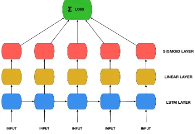
We use a single-layer LSTM model to perform the sequence prediction task, followed by a linear layer that maps to the output vocabulary size. The linear layer is followed by a sigmoid unit layer. The loss is the sum of the mean squared error between the prediction and the correct output at each character. See Figure1for an illustration. In our implementation, we used the standard LSTM module in PyTorch (Paszke et al.,2017) and ini-tialized the initial hidden and cell states, h0 and
c0, to zero.
4 Experimental Setup 4.1 Training and Testing
[image:4.612.320.514.60.193.2]Training and testing are done in alternating steps: In each epoch, for training, we first present to an LSTM network1000samples in a given language, which are generated according to a certain discrete probability distribution supported on a closed fi-nite interval.5We then freeze all the weights in our model, exhaustively enumerate all the sequences in the language by their lengths, and determine 5The strings are presented to the model in a random order.
Figure 1: Our LSTM architecture
the first k shortest sequences whose outputs the model produces inaccurately.6We remark, for the sake of clarity, that our test design is slightly dif-ferent from the traditional testing approaches used byRodriguez et al.(1999);Gers and Schmidhuber
(2001); Rodriguez (2001), since we do not con-sider the shortest sequence in a language whose output was incorrectly predicted by the model, or the largest accepted test set, or the accuracy of the model on a fixed test set.
Our testing approach, as we will see shortly in the following subsections, gives more information about the inductive capabilities of our LSTM net-works than the previous techniques and proves it-self to be useful especially in the cases where the distribution of the length of our training dataset is skewed towards one of the boundaries of the dis-tribution’s support. For instance, LSTM models sometimes fail to capture some of the short se-quences in a language during the testing phase7, but they then predict a large number of long se-quences correctly.8 If we were to report only the shortest sequence whose output our model incor-rectly predicts, we would then be unable to capture the model’s inductive capabilities. Furthermore, we test and report the performance of the model after each full pass of the training set. Finally, in all our investigations, we repeated each experi-ment ten times. In each trial, we only changed the 6In all our experiments, we decided to choosekto be5. 7This phenomenon is usually observed in distributions
where the training set is skewed towards having more long sequences than short sequences.
8We note that correctly predicting the outputs for the
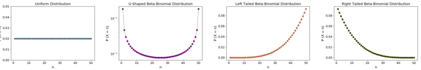
Figure 2: Distributions from Left to Right: Uniform Distribution withN = 50, (U-Shaped) Beta-Binomial
Distri-bution with↵= 0.25, = 0.25, N= 49, (Right-Tailed) Beta-Binomial Distribution with↵= 1, = 5, N= 49,
and (Left-Tailed) Beta-Binomial Distribution with↵= 5, = 1, N= 49.
weights of the hidden states of the model – all the other parameters were kept the same.
4.2 Length Distributions
Previous studies have examined various length distribution models to generate appropriate train-ing sets for each formal language: Wiles and Elman (1995); Bod´en and Wiles (2000); Ro-driguez (2001), for instance, used length distri-butions that were skewed towards having more short sequences than long sequences given a train-ing length-window, whereas Gers and Schmid-huber(2001) used a uniform distribution scheme to generate their training sets. The latter briefly comment that the distribution of lengths of se-quences in the training set does influence the gen-eralization ability and convergence speed9of neu-ral networks, and mention that training sets con-taining abundant numbers of both short and long sequences are learned by networks much more quickly than uniformly distributed regimes. Nev-ertheless, they do not systematically compare or explicitly report their findings. To study the ef-fect of various length distributions on the learning capability and speed of LSTM models, we experi-mented with four discrete probability distributions supported on bounded intervals (Figure2) to sam-ple the lengths of sequences for the languages. We briefly recall the probability distribution functions for discrete uniform and Beta-Binomial distribu-tions used in our data generation procedure. Discrete Uniform Distribution: GivenN 2N, if a random variableX⇠U(1, N), then the prob-ability distribution function ofX is given as fol-lows:
P(x) = (1
N ifx2 {1, . . . , N} 0 otherwise.
9We defineconvergence (learning) speedas the speed at
which a sequence of numbers, thee1ore5values in our cases,
converge to its stationary value.
To generate training data with uniformly dis-tributed lengths, we simply drawnfromU(1, N) as defined above.
Beta-Binomial Distribution: Similarly, given N 2 Z 0 and two parameters↵ and 2 R>0, if a random variableX⇠BetaBin(N, ↵, ), then the probability distribution function ofXis given as follows:
P(x) = ( N
x
B(x+↵,N x+ )
B(↵, ) ifx2 {0, . . . , N}
0 otherwise.
whereB(↵, )is the Beta function. We set differ-ent values of↵and as such in order to generate the following distributions:
U-shaped (↵ = 0.25, = 0.25): The prob-abilities of having short and long sequences are equally high, but the probability of having an average-length sequence is low.
Right-tailed(↵ = 1, = 5): Short sequences are more probable than long sequences.
Left-tailed (↵ = 5, = 1): Long sequences are more probable than short sequences.
4.3 Length Windows
Most of the previous studies trained networks on sequences of lengthsn2[1, N], where typicalN values were between 10 and 50 (Bod´en and Wiles,
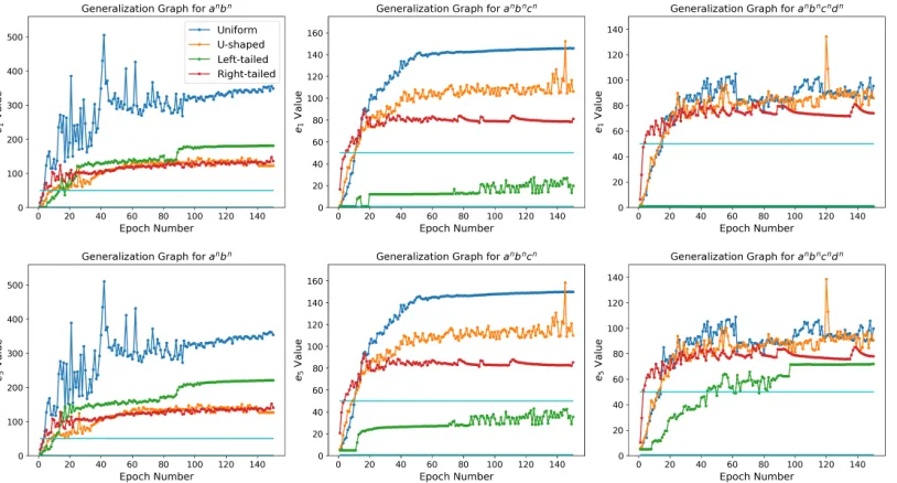
Figure 3: Generalization graphs showing the average performance of LSTMs trained under different probability distribution regimes for each language. The top plots show thee1values, whereas the bottom ones thee5values.
The light blue horizontal lines indicate the training length window[1,50].
4.4 Model Capacity
It has been shown by Gers and Schmidhuber
(2001) that LSTMs can learn anbn and anbncn with1and2hidden units, respectively. Similarly,
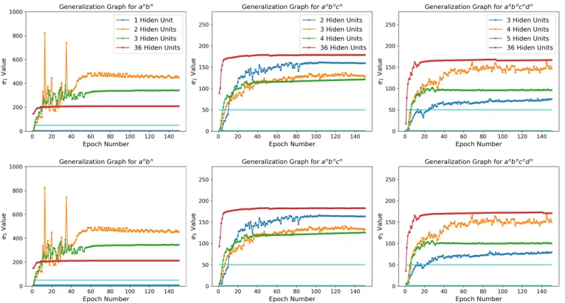
H¨olldobler et al.(1997) demonstrated that a sim-ple RNN architecture containing a single hidden unit with carefully tuned parameters can develop a canonical linear counting mechanism to recognize the simple context-free languageanbn, for n 250. We wanted to explore whether the stability of the networks would improve with an increase in capacity of the LSTM model. We, therefore, varied the number of hidden units in our LSTM models as follows. We experimented with1,2,3, and36hidden units foranbn;2,3,4, and36 hid-den units foranbncn; and3,4,5, and36 hidden units foranbncndn. The36hidden unit case rep-resents an over-parameterized network with more than enough theoretical capacity to recognize all these languages.
5 Results
5.1 Length Distributions
Figure3exhibits the generalization graphs for the three formal languages trained with LSTM models under different length distribution regimes. Each single-color sequence in a generalization graph shows the average performance of ten LSTMs
trained under the same settings but with different weight initializations. In all these experiments, the training sets had the same length-window[1,50]. On the other hand, we used 2, 3, and 4 hidden units in our LSTM architectures for the languages anbn,anbncn, andanbncndn, respectively.10 The top three plots show the average lengths of the shortest sequences (e1) whose outputs were in-correctly predicted by the model at test time, whereas the bottom plots show the fifth such short-est lengths (e5). We note that the models trained on uniformly distributed samples seem to perform the best amongst all the four distributions in all the three languages. Furthermore, for the lan-guagesanbncnandanbncndn, the U-shaped Beta-Binomial distribution appears to help the LSTM models generalize better than the left- and right-tailed Beta Binomial distributions, in which the lengths of the samples are intentionally skewed to-wards one end of the training length-window.
When we look at the plots for the e1 values, we observe that all the distribution regimes seem to facilitate learning at least up to the longest sequences in their respective training datasets, drawn by the light blue horizontal lines on the plots, except for the left-tailed Beta-Binomial dis-tribution for which we see errors at lengths shorter 10The results with other configurations were qualitatively
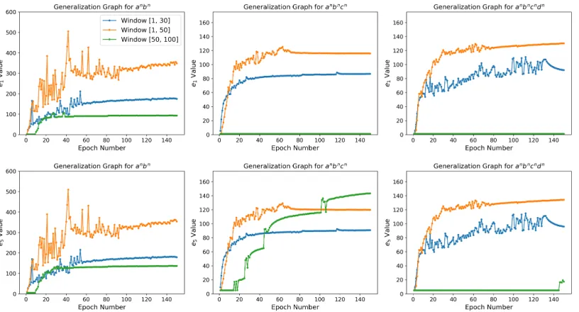
Figure 4: Generalization graphs showing the average performance of LSTMs trained under different training length-windows for each language. The top plots show thee1values, whereas the bottom ones thee5values.
than the training length threshold in the languages anbncn and anbncndn. For instance, if we were to consider only the e1 values in our analysis, it would be tempting to argue that the model trained under the left-tailed Beta-Binomial distri-bution regime did not learn to recognize the lan-guage anbncndn. By looking at the e
5 values, in addition to thee1 values, we however realize that the model was actually learning many of the sequences in the language, but it was just strug-gling to recognize and correctly predict the out-puts of some of the short sequences in the lan-guage. This phenomenon can be explained by the under-representation of short sequences in left-tailed Beta-Binomial distributions. Our observa-tion clearly emphasizes the significance of looking beyonde1, the shortest error length at test time, in order to obtain a more complete picture of the model’s generalizing capabilities.
5.2 Training Length Windows
Figure4shows the generalization graphs for the three formal languages trained with LSTM mod-els under different training windows. We note that enlarging the training length-window, natu-rally, enables an LSTM model to generalize far be-yond its training length threshold. Besides, we see that the models with the training length-window of [50,100] performed slightly better than the other two window ranges in the case ofanbncn (green
line, bottom middle plot). Moreover, we ac-knowledge the capability of LSTMs to recognize longer sequences, as well as shorter sequences. For instance, when trained on the training length-window[50,100], our models learned to recognize not only the longer sequences but also the shorter sequences not presented in the training sets for the languagesanbnandanbncn.
Finally, we highlight the importance of the e5 values once again: If we were to consider only the e1 values, for instance, we would not have captured the inductive learning capabilities of the models trained with a length-window of[50,100] in the case of anbncn, since the models always failed at recognizing the shortest sequenceab in the language. Yet, consideringe5 values helped us evaluate the performance of the LSTM models more accurately.
5.3 Number of Hidden Units
There seems to be a positive correlation between the number of hidden units in an LSTM network and its stability while learning a formal language. As Figure 5 demonstrates, increasing the num-ber of hidden units in an LSTM network both in-creases the network’s stability and also leads to faster convergence. However, it does not necessar-ily result in a better generalization.11 We
conjec-11The results shown in the plot are for models that were
Figure 5: Generalization graphs showing the average performance of LSTM models with a different number of hidden units for each language. The top plots show thee1values, whereas the bottom ones thee5values. The light
blue horizontal lines indicate the training length window[1,50].
ture that, with more hidden units, we simply offer more resources to our LSTM models to regulate their hidden states to learn these languages. The next section supports this hypothesis by visualiz-ing the hidden state activations durvisualiz-ing sequence processing.
6 Discussion
In addition to the analysis of our empirical re-sults in the previous section, we would like to touch upon two important characteristics of LSTM models when they learn formal languages, namely the convergence issue and counting behavior of LSTM models.
Convergence: We note that our experiments in-dicate that LSTM models often do not general-ize to the same value in a given experiment set-ting. Figure 6, for instance, displays the gener-alization and loss graphs of LSTM models which were trained to recognize the languageanbncn un-der a uniform distribution regime with a training window of[1,50]. The figure shows the results of 10 trials with different random weight initializa-tions. While all runs appear to converge to a sim-ilar loss value, they have different generalization values (that is, theire1 values are all different). length window of[1,50]. We observed similar trends with other configurations.
This pattern is fairly common in our experiments, suggesting a disconnection between loss conver-gence and generalization capability. This result again highlights the importance of performing a fine-grained evaluation of generalization capabil-ity, rather than reporting a single number. Our argument is also consistent with those ofBod´en and Wiles (2002) and Chalup and Blair (2003), for they also found that the weight initialization affects the inductive capabilities of an LSTM.
Counting Behavior: Here we look at the acti-vation dynamics of the hidden states of the model when processing specific sequences. Figure 7
demonstrates that an LSTM network organizes its hidden state structure in such a way that certain hidden state units learn how to count up and down upon the subsequent encounter of some characters. In the case ofa100b100c100d100, we observe, for in-stance, that certain units get activated at time steps 100,200, and 300. In fact, some units appear to cooperate together to count.
sam-Figure 6: Generalization graph (left) and loss graph (right) with different random weight initializations.
Figure 7: Hidden state dynamics in a four-unit LSTM model. We note that certain units in the LSTM model get activated at time steps100,200, and300.
ple. It simply outputs(a/b)1000b996a4, instead of (a/b)1000b999 a. Our results corroborate and re-fine the findings ofGers and Schmidhuber(2001) andWeiss et al.(2018), who noted the existence of a counting mechanisms for simpler languages, while we also observe a collaborative counting be-havior in over-parameterized networks.
7 Conclusion
In this paper, we have addressed the influ-ence of various length distribution regimes and length-window sizes on the generalizing ability of LSTMs to learn simple free and context-sensitive languages, namely anbn, anbncn, and anbncndn. Furthermore, we have discussed the ef-fect of the number of hidden units in LSTM mod-els on the stability of a representation learned by the network: We show that increasing the num-ber of hidden units in an LSTM model improves the stability of the network, but not necessarily the
inductive power. Finally, we have exhibited the importance of weight initialization to the conver-gence of the network: Our results indicate that ferent hidden weight initializations can yield dif-ferent convergence values, given that all the other parameters are unchanged. Throughout our anal-ysis, we emphasized the importance of a fine-grained evaluation, considering generalization be-yond the first error and during training. We there-fore concluded that there are an abundant number of parameters that can influence the inductive abil-ity of an LSTM to learn a formal language and that the notion of learning, from a neural network’s perspective, should be treated carefully.
8 Acknowledgment
[image:9.612.97.286.263.389.2]References
Dana Angluin. 1980. Inductive inference of formal languages from positive data. Information and con-trol, 45(2):117–135.
Dzmitry Bahdanau, Kyunghyun Cho, and Yoshua Ben-gio. 2014. Neural machine translation by jointly learning to align and translate. arXiv preprint arXiv:1409.0473.
Mikael Bod´en and Janet Wiles. 2000. Context-free and context-sensitive dynamics in recurrent neural net-works.Connection Science, 12(3-4):197–210.
Mikael Bod´en and Janet Wiles. 2002. On learning context-free and context-sensitive languages. IEEE Transactions on Neural Networks, 13(2):491–493. Mike Casey. 1996. The dynamics of discrete-time
computation, with application to recurrent neural networks and finite state machine extraction. Neu-ral computation, 8(6):1135–1178.
Stephan K Chalup and Alan D Blair. 2003. Incremen-tal training of first order recurrent neural networks to predict a context-sensitive language. Neural Net-works, 16(7):955–972.
Sreerupa Das, C Lee Giles, and Guo-Zheng Sun. 1992. Learning context-free grammars: Capabilities and limitations of a recurrent neural network with an ex-ternal stack memory. InProceedings of The Four-teenth Annual Conference of Cognitive Science So-ciety. Indiana University, page 14.
Jeffrey L Elman. 1991. Distributed representations, simple recurrent networks, and grammatical struc-ture.Machine learning, 7(2-3):195–225.
Felix A Gers and E Schmidhuber. 2001. LSTM recur-rent networks learn simple free and context-sensitive languages. IEEE Transactions on Neural Networks, 12(6):1333–1340.
C Lee Giles, Clifford B Miller, Dong Chen, Hsing-Hen Chen, Guo-Zheng Sun, and Yee-Chun Lee. 1992. Learning and extracting finite state automata with second-order recurrent neural networks. Neu-ral Computation, 4(3):393–405.
Klaus Greff, Rupesh K Srivastava, Jan Koutn´ık, Bas R Steunebrink, and J¨urgen Schmidhuber. 2017. LSTM: A search space odyssey. IEEE transac-tions on neural networks and learning systems, 28(10):2222–2232.
Sepp Hochreiter and J¨urgen Schmidhuber. 1997. Long short-term memory. Neural computation, 9(8):1735–1780.
Steffen H¨olldobler, Yvonne Kalinke, and Helko Lehmann. 1997. Designing a counter: Another case study of dynamics and activation landscapes in re-current networks. InAnnual Conference on Artifi-cial Intelligence, pages 313–324. Springer.
Stan C Kwasny and Barry L Kalman. 1995. Tail-recursive distributed representations and simple re-current networks.Connection Science, 7(1):61–80. Nelson F. Liu, Omer Levy, Roy Schwartz, Chenhao
Tan, and Noah A. Smith. 2018. LSTMs Exploit Linguistic Attributes of Data. In Proceedings of the Third Workshop on Representation Learning for NLP.
Adam Paszke, Sam Gross, Soumith Chintala, Gre-gory Chanan, Edward Yang, Zachary DeVito, Zem-ing Lin, Alban Desmaison, Luca Antiga, and Adam Lerer. 2017. Automatic differentiation in PyTorch. InNIPS-W.
Paul Rodriguez. 2001. Simple recurrent networks learn context-free and context-sensitive languages by counting. Neural computation, 13(9):2093– 2118.
Paul Rodriguez, Janet Wiles, and Jeffrey L. Elman. 1999. A Recurrent Neural Network that learns to count.Connection Science, 11(1):5–40.
Hasim Sak, Andrew W. Senior, and Franc¸oise Bea-ufays. 2014. Long short-term memory recurrent neural network architectures for large scale acoustic modeling. In15th Annual Conference of the Inter-national Speech Communication Association (Inter-speech), pages 338–342.
Hava T Siegelmann. 1995. Computation beyond the Turing limit.Science, 268(5210):545–548.
Hava T Siegelmann and Eduardo D Sontag. 1992. On the computational power of neural nets. In Proceed-ings of the fifth annual workshop on Computational learning theory, pages 440–449. ACM.
Mark Steijvers and Peter Gr¨unwald. 1996. A recurrent network that performs a context-sensitive prediction task. InProceedings of the 18th annual conference of the cognitive science society, pages 335–339. Ilya Sutskever, Oriol Vinyals, and Quoc V. Le. 2014.
Sequence to Sequence Learning with Neural Net-works. InAdvances in neural information process-ing systems, pages 3104–3112.
Gail Weiss, Yoav Goldberg, and Eran Yahav. 2018.On the practical computational power of finite precision rnns for language recognition. InProceedings of the 56th Annual Meeting of the Association for Compu-tational Linguistics (Volume 2: Short Papers), pages 740–745. Association for Computational Linguis-tics.