Learning to Recognize Animals by Watching Documentaries: Using Subtitles as Weak Supervision

Learning to Recognize Animals by Watching Documentaries:

Using Subtitles as Weak Supervision

Aparna Nurani Venkitasubramanian1_{, Tinne Tuytelaars}2_{, and Marie-Francine Moens}1 1_{KU Leuven, Computer Science Department, Belgium}

2_{KU Leuven, ESAT-PSI, IMEC, Belgium}

{firstname.lastname}@kuleuven.be

Abstract

We investigate animal recognition models learned from wildlife video documentaries by using the weak supervision of the tex-tual subtitles. This is a challenging setting, since i) the animals occur in their natural habitat and are often largely occluded and ii) subtitles are to a great degree comple-mentary to the visual content, providing a very weak supervisory signal. This is in contrast to most work on integrated vision and language in the literature, where tex-tual descriptions are tightly linked to the image content, and often generated in a curated fashion for the task at hand. We investigate different image representations and models, in particular a support vec-tor machine on top of activations of a pre-trained convolutional neural network, as well as a Naive Bayes framework on a ‘bag-of-activations’image representation, where each element of the bag is consid-ered separately. This representation al-lows key components in the image to be isolated, in spite of vastly varying back-grounds and image clutter, without an ob-ject detection or image segmentation step. The methods are evaluated based on how well they transfer to unseen camera-trap images captured across diverse topograph-ical regions under different environmen-tal conditions and illumination settings, in-volving a large domain shift.

1 Introduction

It is estimated1 _{that video traffic will be 82} per-cent of all global Internet traffic by 2020. The

1

http://www.cisco.com/c/en/us/solutions/collateral/service- provider/visual-networking-index-vni/complete-white-paper-c11-481360.html

ubiquitousness of video on the web demands in-dexing tools that facilitate fast and easy access to relevant content. Traditionally, video search has been based on user-tags. However, in the recent past, research activities have been directed at au-tomatic indexing of videos based on the content. Contributing to this goal of automatic video index-ing, we focus on the problem of wildlife recogni-tion in nature documentaries with subtitles.

This setup is challenging from at least two per-spectives: first, from the point of view of the con-tent, and second, due to thenature of video docu-mentaries. As far as the contentis concerned, we are dealing with animals shot in their natural habi-tat. The problem of identifying animals in videos, especially those shot in the natural habitat presents several challenges. Firstly, animals are among the most difficult objects to recognize in images and videos, mainly due to their deformable bodies that often self occlude and the large variation they pose in appearance and depiction (Afkham et al.,2008;

Berg and Forsyth, 2006). Further, in the natural habitat, there are challenges due to camouflage and occlusion by flora. Moreover, unlike faces or cuboidal objects such as furniture, we do not have accurate detectors that can localize the an-imal in a frame. State-of-the-art object proposal methods such as (Girshick et al.,2014;Ren et al.,

2015) yield an unacceptably low level of either re-call or precision. The absence of detectors neces-sitates other mechanisms that allow segregation of the components of the image.

Thenature of video documentariespresents yet another challenge. Typically, in video documen-taries such as ours, the subtitles are not parallel, but complementary to the visuals (See Fig. 1). This is in contrast to most work on integrated vi-sion and language in the literature, where textual descriptions are tightly linked to the image con-tent. This means we do not have examples that

In the rivers and lakes of Africa, lives an animal which has a reputation for being the most unpredictable and dangerous of all.

Evencrocodilesare wary. Thehippopotamus.

Figure 1: A set of frames together with the corresponding subtitles: The frames show hippos, while the subtitles mention both hippo and crocodile.

can reliably tie together textual and visual entities. In this work, we study image representations and models that cope with the above challenges. These include a support vector machine on top of activations of a pretrained convolutional neu-ral network, and a Naive Bayes framework on a ‘bag-of-activations’ image representation, where each element of the bag is considered separately. While the former utilizes aglobal representation denoted by the feature vector comprising CNN ac-tivations, the latter works on per dimension ba-sis, allowing key components in the image to be isolated, in spite of largely varying backgrounds and image clutter, without an object detection or image segmentation step. We experiment with both continuous and discretized variants of the ‘bag-of-activations’representation. In particular, we investigate image representations and weakly supervised animal recognition models that can be learned without the need for bounding boxes, or curated data comprising manually annotated training examples.

The rest of this paper is organized as follows: Section 2 presents the background and related work. Section 3provides the problem definition. Section4describes the image representations and animal recognition models based on CNN activa-tions. Section5discusses the experiments and re-sults. Finally, Section6provides the conclusions.

2 Related Work

Identifying animals is a well-studied topic (Afkham et al., 2008; Berg and Forsyth, 2006;

Schmid, 2001; Ramanan et al., 2006). Recent

works such as (Hariharan and Girshick,2016) and (Gomez and Salazar,2016) advance us further and provide better insight into the problem. However, these methods are not applicable in our setting since they require extensive training data. It is important to note that in this setup, we lack suffi-cient reliable training data making neural network-based training impractical.

Apart from these works that focus specifically on animals, there is a large literature on generic object detection. These methods are often evalu-ated on the Pascal VOC challenge dataset ( Ever-ingham et al.,2012) which includes classes of an-imals such as cats, dogs, cows and horses, among other things. There are also datasets that focus on animals such as Caltech UCSD Birds (Wah et al., 2011) and Stanford Dogs (Khosla et al.,

2011). Additionally, the FishClef and BirdClef challenges which are part of LifeClef (Joly et al.,

2015) provide an arena for identification of species of fish and birds respectively. Most of these datasets are, however, object-centered and in that sense easier than the ‘in-the-wild’ setting we are dealing with.

of animals may not be found on ImageNet. Recently, there has been considerable interest in sentence/caption generation from images as well as natural language based object detection, e.g. (Karpathy and Fei-Fei, 2014; Fang et al.,

2014;Guadarrama et al.,2013;Kazemzadeh et al.,

2014). These approaches typically rely on text snippets that accurately describe the content of the images or videos. However, in our context, the subtitles and the visuals are not parallel, but com-plementary. For example, often a few animals are mentioned in the text, while the connected frame only shows one of them. The connection between the vision and the text is therefore much weaker. Additionally, in our setup, we have too few data to train similar models. As a result, these approaches are not directly applicable to our setting. In this paper, we explore weakly-supervised models that can deal with the complementarity or the ‘non-parallelism’ of the visual and textual modalities.

There has also been some work on alignment across modalities for recognizing people (Pham et al.,2010,2011;Guillaumin et al.,2008). These approaches rely on the use of a face-detector. While there are face detectors available with rea-sonable accuracy, there are no such detectors that allow localizing animals. The absence of the bounding boxes complicates the problem in many ways. A notable endeavor in this domain is that of (Everingham et al.,2006) where dialogue tran-scripts and other supervisory information (such as lip movements or clothing) are used in addition to subtitles and face detectors. In our context, since the subjects of our videos involve animals, cues such as lip movements or clothing are not relevant. In this paper, we investigate image representa-tions and multi-modal animal recognition models that can cope with a) complementarity of vision and language, b) lack of bounding boxes and c) lack of labeled external data, and can transfer to a different unseen domain, shot under very different conditions.

3 Task definition

We have a wildlife documentary with subti-tles. On the visual side, we derive key frames

F = {f1, f2. . . fq} from which we extract vi-sual features with a suitable representation A =

{a1,a2. . .aq}. Assume each feature vector has

D dimensions. On the textual side, from the sub-titles, we identify theuniqueanimal mentions or

animal names N = {n1, n2. . . np}, using a list of animal names derived from WordNet (Miller,

1995) as in (Dusart et al.,2013).

Using the setup of (Venkitasubramanian et al.,

2016), we associate every framefi,1 ≤ i ≤ q, with a setNi ⊂ Nof possible animal names de-rived from 5 subtitles to the left and right of the frame. The setNi refers to the set of unique ani-mal names derived from their mentions and coref-erences in the subtitles2_{. It is possible that the} frame has some or all or none of the animals in Ni. Corresponding to every name nl ∈ Ni, we have a binary label yl indicating the presence or absence of nl. Our objective is to find the most likely value ofylcorresponding to namenl ∈Ni for every framefi.

4 Image Representations Based on CNN Activations

A popular choice of visual features for object recognition is the activations of the penultimate layer of a pretrained Convolutional Neural Net-work. In this work, we use the VGG CNN-M-128 architecture3 _{of (Chatfield et al., 2014), which is} trained on 1,000 object categories from ImageNet (Deng et al.,2009) with roughly 1.2M training im-ages. Within this realm, we explore two perspec-tives on the real-valued feature vector: (i) aglobal representationwhere each feature vector is treated as one entity, and (ii) a bag-of-activations repre-sentation, where each element of the bag is con-sidered separately.

The global representation is by far the most

commonly used (Sharif Razavian et al.,2014) and fits well with a linear Support Vector Machine (SVM) classifier. For the task of object recogni-tion, the linear SVM is typically used with theL2 norm, and has the following objective function

minimize

wl

1

2||wl||2+C X

i

max(1−ylwlTai,0)

wherewldenotes the set of weights to be learned

for the label yl corresponding to name nl, and C denotes the cost4_{. In a weakly supervised} setting, these weights are learned based on the

2_{There remains a small percentage (2.35%) of animals not}

mentioned in the nearby subtitles. These will be left unde-tected.

3_{This model yielded 128 features.}

4_{We used the Liblinear (Fan et al.,2008) toolkit, with the}

weakly associated (hence noisy) frame-name pairs <ai, nl >for allnl∈Ni.

An alternative to this global representation is

a bag-of-activations representation, where each

feature dimension is treated in isolation. Li et al. (2014) have shown that the CNN activations have two interesting properties: firstly, they can be treated independently along the dimensions and second, they preserve their essence even after bi-narization. We exploit the first property and use it in a naive Bayes framework. The idea of treat-ing each element of the CNN representation indi-vidually rather than using the full feature vector in a high-dimensional space is crucial: It brings robustness to image clutter and changing back-grounds, and helps in learning from few examples.

p(yl|ai) = p(yl)

Q_D

v=1p(aiv|yl)

Zl (1)

Zl is a normalization constant for the name nl, given by

Zl =p(yl) D Y

v=1

p(aiv|yl)+p(yl) D Y

v=1

p(aiv|yl) (2)

whereyl = 0 ifyl = 1 and vice versa. p(yl)is the prior which we assume to be uninformative for simplicity. So,p(yl= 0) =p(yl= 1).

Then, using Eq. 2, Eq. 1 can be written as fol-lows:

p(yl|ai) =

Q_D

v=1p(aiv|yl) Q_D

v=1p(aiv|yl) +QDv=1p(aiv|yl) (3) The second interesting property of the CNN ac-tivations is that they preserve their essence even after binarization. We investigate this further and show that not only binarization but also

dis-cretizationof the feature vector into a larger

num-ber of bins is useful. In particular, we propose to discretize the feature vector into B bins along each dimension5_{. In this paper, we experiment with} two approaches for binning the feature vector - (i) equal width and (ii) equal frequency. The equal width approach ensures that all the bins are of the same size. For example, if we are interested in 2 equal width bins, we could look at the feature vec-tor along a dimension and set the threshold mid-way between the minimum and maximum values

5_{Discretization can also be applied to theglobal}

repre-sentationused by the SVM, but as shown in ( Venkitasubra-manian et al.,2016), it is particularly useful in conjunction with a naive Bayes classifier.

of that dimension. The values that are less than the threshold could be set to 0, while the rest are set to 1. In equal frequency binning, the threshold is set such that the number of elements in each bin is roughly the same.

This discretization is similar to the vector quan-tization of SIFT descriptors to obtain Bag of Vi-sual Words (BoVW). But, while BoVW has the issue that the discretization errors can have a sig-nificant negative impact, with CNN features,there are no strong discretization artifacts. In fact, Li et al. (2014) have shown that retaining just the values of the largestkdimensions (or even setting the val-ues of the largestkdimensions to 1 and the rest to 0) is sufficient to capture the essence of the image. Discretizing the feature space allows us to re-place the featureaivby the corresponding binβv.

p(aiv|yl) =p(βv|yl) (4) where βv ∈ {0,1. . . B} is the bin to which aiv belongs.

Eq. 3 can then be rewritten as

p(yl|ai) =

Q_D

v=1p(βv|yl) Q_D

v=1p(βv|yl) +QDv=1p(βv|yl) (5) To compute the conditional probabilities p(βv|yl) of the bin βv given yl, we rely on the noisy labels that can be obtained from the text. Basically we count the co-occurrence of label yl corresponding to name nl ∈ Ni with bin βv relative to the total number of instances whereyl occurs in our dataset.

p(βv|yl) = freq_freq(β₍v_y, yl)

l) (6)

5 Experiments and Results

The dataset used in our experiments is that of (Dusart et al.,2013). This is a wildlife documen-tary named ‘Great Wildlife Moments’6 _with sub-titles from the BBC. This is an interlaced video with a duration of 108 minutes at a frame rate of 25 frames per second, and the frame resolution is 720x576 pixels. The video consists of 28 chap-ters and all the chapchap-ters except the ones contain-ing just one animal are evaluated. This leaves us with chapters 14 to 28. Applying shot cut detec-tion (Hellier et al.,2012) on these chapters, we ob-tained 602 key frames. Of these, 302 frames had

Method Precision Recall F1

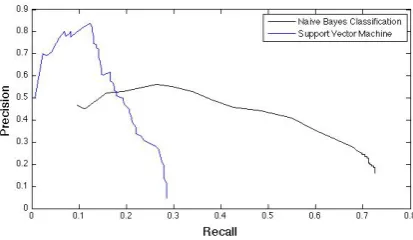
SVM 80.43 12.71 21.96

Naive Bayes 20.23 71.48 31.54 Table 1: Results of using thecontinuous features and applying the weak labels of our dataset

Figure 2: The precision-recall curves for the SVM and naive Bayes classifier shown in Table1. Area under the curve is 0.1599 for the SVM and 0.3642 for naive Bayes.

no animal. The remaining 300 contained 365 ani-mals in total. We run our algorithm on all the 602 key frames. There were 19 species of animals.

The animal labeling is evaluated in terms of precision, recall andF1 computed over the entire dataset as follows:

precision= number of labels correctly assigned_{total number of labels assigned}

recall= number of labels correctly assigned_{actual number of animal present}

The evaluation covers two aspects:

1. How well do the representation and model learned using the weak labels of our dataset perform on the same dataset? (Section5.1) 2. How well do the representation and model

learned using the weak labels of our dataset transfer to an external dataset shot over di-verse topographical regions under different environmental conditions and illumination settings? (Section5.2)

5.1 Animal labeling on wildlife videos

Table1shows the performance of an SVM on the global representationand a naive Bayes classifier on the bag of activations using continuous fea-tures. In either case, namenlis assigned to frame

Figure 3: The distribution of the feature val-ues along the first dimension: x-axis shows the range of feature values, y-axis shows the num-ber of frames. The grey histogram shows the distribution of the feature values. The red curve is the normal distribution plotted using the mean and standard deviation along the first dimension,

N(0.0454,0.0622).

ai ifp(yl|ai) > p(yl|ai), that is, the probability

threshold for prediction was set at 0.5. For the naive Bayes classifier, a Gaussian distribution was used to model the continuous features along each dimension. While both models do not yield ade-quate performance, the naive Bayes certainly does far better compared to the SVM. In this setup in-volving limited reliable example pairs,it is benefi-cial to treat each element of the CNN representa-tion individually rather than using the full feature vector in a high-dimensional space. Fig.2shows the precision-recall curves of the SVM and the naive Bayes classifier. The naive Bayes is clearly better in this setup, except in the low recall / high precision region.

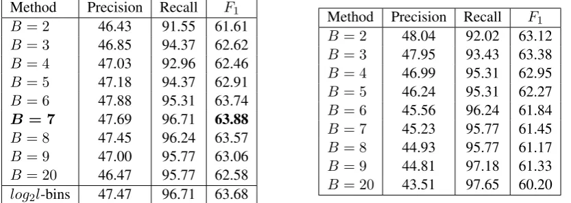
Method Precision Recall F1 B= 2 46.43 91.55 61.61 B= 3 46.85 94.37 62.62 B= 4 47.03 92.96 62.46 B= 5 47.18 94.37 62.91 B= 6 47.88 95.31 63.74

B = 7 47.69 96.71 63.88

B= 8 47.45 96.24 63.57 B= 9 47.00 95.77 63.06 B= 20 46.47 95.77 62.58 log2l-bins 47.47 96.71 63.68

Method Precision Recall F1 B = 2 48.04 92.02 63.12 B = 3 47.95 93.43 63.38 B = 4 46.99 95.31 62.95 B = 5 46.24 95.31 62.27 B = 6 45.56 96.24 61.84 B = 7 45.23 95.77 61.45 B = 8 44.93 95.77 61.17 B = 9 44.81 97.18 61.33 B = 20 43.51 97.65 60.20

Table 2: Results of using thediscretized features(left: equal width discretization, right: equal frequency discretization) and applying the weak labels of our dataset

Next, we present the results of using the dis-cretized features. Table2 (left) shows the results of the animal labeling using equal width binning for different number of bins B. First, we use a fixed number of bins over every dimension. That is, along every dimension in the feature vector, the number of bins is set to a constant B. Note that irrespective of the number of bins, the per-formance has improved significantly. The preci-sion has more than doubled, and the recall has improved by more than 20% absolute. Contrary to expectations, the discretization has actually im-proved the classification. These findings are con-sistent with those of Dougherty et al. (Dougherty et al.,1995). Overall, we see that these results are significantly better than all the baselines in Table

1. In addition to the discretization, the key as-pects of this method are the use of naive Bayes classifier and the idea of treating each element of the CNN representation separately rather than us-ing the full feature vector in a high-dimensional space. These bring robustness to image clutter and changing backgrounds, and help in learning from few examples.

Next, looking at the F1 measures for different values of B, we see that the best results are ob-tained when B = 7. In addition to fixing the number of bins along every dimension, we used a heuristic to set a variable number of bins for each dimension. Using the heuristic in S-Plus his-togram algorithm of Spector (Spector,1994), we set the number of bins along each dimension to log2l, where l is the number of unique values in that dimension. Using this heuristic, different di-mensions had different number of bins. We ob-served that of the 128 dimensions, 12 had 7 bins,

while the rest had 8 bins. This explains why we have the best results in the range B = 7 and B = 8.

Table 2(right) shows the results of the animal labeling using equal frequency binning for differ-ent number of binsB. Here, since we are deal-ing with sparse matrices, we have to ensure that all zero-valued entries along a dimension should belong to the same bin. The results in table2 in-corporate this correction. As with the equal-width case, we obtain significant improvements over the naive Bayes classifier with continuous features.

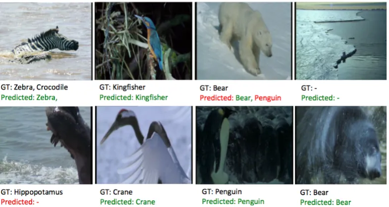
Fig.4shows some of the sample outputs of our system. Note that our method is capable of iden-tifying multiple species in the same frame, as well as detecting frames that do not contain any animal.

5.2 Transfer to camera-trap images

The second aspect of the evaluation is to measure how well the representations and models transfer to external data from an entirely different setup. To evaluate this, we use the Snapshot Serengeti (Swanson et al.,2015) dataset, which consists of camera-trap (remote, automatic cameras) images covering wildlife in Savanna. We learn animal recognition models using the weak labels of our dataset and apply them to the Snapshot Serengeti (Swanson et al.,2015) dataset. It is important to note that the pictures of this Serengeti dataset are captured automatically, in very different scenes, under various illumination conditions. This causes a hugedomain shift. The Serengeti dataset covers 40 mammalian species, of which three (Lion, Ze-bra and Hippopotamus) also appear in our dataset. We choose 500 random images7_{each of Lion and}

Figure 4: Some sample outputs from our system. ‘GT’ indicates ground truth, ‘Predicted’ indicates the predictions of the system.

Zebra, and all 37 images available for the Hip-popotamus class. This set forms the target data on which the animal recognition models will be tested. Fig. 5 shows some of the sample images from this dataset.

Table 3 shows the performance of the animal recognition models learned using our data, applied on the target dataset. The first baseline is simply based on the probabilities output by the CNN pre-trained on ImageNet. We used the same architec-ture (CNN-M-128) that was used for feaarchitec-ture ex-traction. When the output probability for a certain class was >0.5, we concluded that the system pre-dicted that class. Of course, multiple classes could be predicted for each key frame. Although some of the classes predicted covered ‘lake side’, ‘hay’ etc. which were not explicitly labeled in our setup, there were a lot of animals incorrectly predicted (which did not belong to our dataset of 19 ani-mals). These included elephant, panther, camel, dugong. We filtered the outputs to just retain the 19 classes that were seen in our dataset. This in-creased the precision by a large margin (second row in the table). Next, we retained only the three classes that were common to our dataset and Serengeti dataset. While this gave a perfect preci-sion, the recall stands low at approx. 20% in all the three cases above.

Next, we train an SVM (on the continuous fea-tures) on all the 19 classes of our dataset, using the weak association of the subtitles and applied them to Serengeti (Swanson et al., 2015) dataset

(Second block on table 3). Note that the perfor-mance is low compared to ImageNet cases in the first block. The model learned by the SVM on our dataset does not compare well with that of Im-ageNet, which was trained on several thousands of zebra, hippos and lions. As with the previ-ous block, filtering to the 3 relevant classes in-creases the precision by a large margin, while the recall stays the same. When we used the ground truth labels instead of the weak labels (which ba-sically indicate if a frame could have some ani-mal), we have a perfect precision, but the recall is even lower. By capturing elements in the back-ground/environment which might be related to the animal, (e.g., a water body for the hippopotamus, or grasslands for the zebra), the training based on weak labels yields higher recall, albeit at the cost of precision.

Figure 5: Some sample images from the Snapshot Serengeti (Swanson et al., 2015) dataset, together with the descriptions that show the difficulty of the task. Green box indicates the animal was recognized correctly, while red indicates the animal was missed.

Method Precision Recall F1

CNN-M-128 (1000 classes) 21.98 20.38 21.15

CNN-M-128 (filtered to 19 classes of our dataset) 91.75 20.38 33.35 CNN-M-128 (filtered to 3 overlapping classes) 100 20.38 33.86 SVM continuous (on our 19 classes) - using weak labels 58.16 14.96 23.80 SVM continuous (on 3 overlapping classes) - using weak labels 86.34 14.96 25.50 SVM continuous (on 3 overlapping classes) - using GT 100 9.31 17.04 NBC continuous (on 3 overlapping classes) - using weak labels 49.03 90.53 63.61 NBC continuous (on 3 overlapping classes) - using GT 62.07 67.71 64.77 NBC discretized intolog2lbins (on 3 classes) - using weak labels 53.45 65.73 58.95 Table 3: Performance of the animal recognition models learned using our data, applied on images from Snapshot Serengeti (Swanson et al.,2015) dataset

transfer as well to the target domain. Neverthe-less, it certainly outperforms the classifiers in the first two blocks, by a large margin.

6 Conclusions

In this paper, we investigate different image rep-resentations and models, including a support vec-tor machine on top of activations of a pretrained convolutional neural network, as well as a Naive Bayes framework on a bag-of-activations image representation, where each element of the bag is considered separately. We show that the bag-of-activationsrepresentation allows key components in the image to be isolated, in spite of largely vary-ing backgrounds and image clutter, and eliminates the need for an object detection or image segmen-tation step.In contrast to most work on integrated vision and language that use curated data, the

pro-posed approach deals with vision and language that are complementary.

References

Heydar Maboudi Afkham, Alireza Tavakoli Targhi, Jan-Olof Eklundh, and Andrzej Pronobis. 2008. Joint visual vocabulary for animal classification. In

19th International Conference on Pattern Recogni-tion. IEEE, pages 1–4.

Tamara L. Berg and David A. Forsyth. 2006. Animals on the web. InIEEE Computer Society Conference on Computer Vision and Pattern Recognition. IEEE, volume 2, pages 1463–1470.

Ken Chatfield, Karen Simonyan, Andrea Vedaldi, and Andrew Zisserman. 2014. Return of the devil in the details: Delving deep into convolutional nets. In Proceedings of the British Machine Vision Confer-ence.

Jia Deng, Wei Dong, Richard Socher, Li-Jia Li, Kai Li, and Li Fei-Fei. 2009. Imagenet: A large-scale hierarchical image database. In IEEE Conference on Computer Vision and Pattern Recognition. IEEE, pages 248–255.

James Dougherty, Kohavi Ron, and Sahami Mehran. 1995. Supervised and unsupervised discretization of continuous features. InProceedings of the twelfth international conference on Machine Learning. San Francisco, CA: Morgan Kaufmann, volume 12, page 194–202.

Thibaut Dusart, Aparna Nurani Venkitasubramanian, and Marie-Francine Moens. 2013. Cross-modal alignment for wildlife recognition. InProceedings of the 2nd ACM International Workshop on Multi-media Analysis for Ecological Data. ACM, pages 9–14.

Mark Everingham, Josef Sivic, and Andrew Zisserman. 2006. Hello! my name is... buffy”–automatic nam-ing of characters in tv video. In Proceedings of the British Machine Vision Conference. volume 2, page 6.

Mark Everingham, Luc Van Gool, Cristopher K. I. Williams, John Winn, and Andrew Zisserman. 2012. The PASCAL Visual Object Classes Challenge 2012 (VOC2012) Results.

Rong-En Fan, Kai-Wei Chang, Cho-Jui Hsieh, Xiang-Rui Wang, and Chih-Jen Lin. 2008. Liblinear: A library for large linear classification. Journal of Ma-chine Learning Research9:1871–1874.

Hao Fang, Saurabh Gupta, Forrest Iandola, Rupesh Sri-vastava, Li Deng, Piotr Dollár, Jianfeng Gao, Xi-aodong He, Margaret Mitchell, John Platt, et al. 2014. From captions to visual concepts and back.

arXiv preprint arXiv:1411.4952.

Ross Girshick, Jeff Donahue, Trevor Darrell, and Jiten-dra Malik. 2014. Rich feature hierarchies for accu-rate object detection and semantic segmentation. In

Proceedings of the IEEE Conference on Computer Vision and Pattern Recognition. pages 580–587.

Alexander Gomez and Augusto Salazar. 2016. To-wards automatic wild animal monitoring: Identifi-cation of animal species in camera-trap images us-ing very deep convolutional neural networks. arXiv preprint arXiv:1603.06169.

Sergio Guadarrama, Niveda Krishnamoorthy, Girish Malkarnenkar, Subhashini Venugopalan, Raymond Mooney, Trevor Darrell, and Kate Saenko. 2013. Youtube2text: Recognizing and describing arbitrary activities using semantic hierarchies and zero-shot recognition. In IEEE International Conference on Computer Vision. IEEE, pages 2712–2719.

Matthieu Guillaumin, Thomas Mensink, Jakob Ver-beek, and Cordelia Schmid. 2008. Automatic face naming with caption-based supervision. In IEEE Conference on Computer Vision and Pattern Recog-nition. IEEE, pages 1–8.

Bharath Hariharan and Ross Girshick. 2016. Low-shot visual object recognition. arXiv preprint arXiv:1606.02819.

Pierre Hellier, Vincent Demoulin, Lionel Oisel, and Patrick Pérez. 2012. A contrario shot detection. In

19th IEEE International Conference on Image Pro-cessing. IEEE, pages 3085–3088.

Alexis Joly, Hervé Goëau, Hervé Glotin, Concetto Spampinato, Pierre Bonnet, Willem-Pier Vellinga, Robert Planqué, Andreas Rauber, Simone Palazzo, Bob Fisher, et al. 2015. Lifeclef 2015: multime-dia life species identification challenges. In Inter-national Conference of the Cross-Language Eval-uation Forum for European Languages. Springer, pages 462–483.

Andrej Karpathy and Li Fei-Fei. 2014. Deep visual-semantic alignments for generating image descrip-tions.arXiv preprint arXiv:1412.2306.

Sahar Kazemzadeh, Vicente Ordonez, Mark Matten, and Tamara L. Berg. 2014. Referit game: Referring to objects in photographs of natural scenes. In Pro-ceedings of the Conference on Empirical Methods in Natural Language Processing.

Aditya Khosla, Nityananda Jayadevaprakash, Bang-peng Yao, and Fei-fei Li. 2011. Novel dataset for fine-grained image categorization. In First Work-shop on Fine-Grained Visual Categorization, IEEE Computer Society Conference on Computer Vision and Pattern Recognition. Citeseer.

Yao Li, Lingqiao Liu, Chunhua Shen, and Anton van den Hengel. 2014. Mid-level deep pattern min-ing.arXiv preprint arXiv:1411.6382.

George A. Miller. 1995. WordNet: A lexical database for English. Communications of the ACM38:39–41. Phi The Pham, Marie-Francine Moens, and Tinne Tuytelaars. 2010. Cross-media alignment of names and faces. IEEE Transactions on Multimedia

Phi The Pham, Tinne Tuytelaars, and Marie-Francine Moens. 2011. Naming people in news videos with label propagation. IEEE Multimedia18(3):44–55. Deva Ramanan, David A Forsyth, and Kobus Barnard.

2006. Building models of animals from video.

IEEE Transactions on Pattern Analysis and Machine Intelligence,28(8):1319–1334.

Shaoqing Ren, Kaiming He, Ross Girshick, and Jian Sun. 2015. Faster R-CNN: Towards real-time ob-ject detection with region proposal networks. In Ad-vances in Neural Information Processing systems. pages 91–99.

Cordelia Schmid. 2001. Constructing models for content-based image retrieval. InProceedings of the IEEE Computer Society Conference on Computer Vision and Pattern Recognition,. IEEE, volume 2, pages II–39.

Ali Sharif Razavian, Hossein Azizpour, Josephine Sul-livan, and Stefan Carlsson. 2014. CNN features off-the-shelf: an astounding baseline for recognition. In

Proceedings of the IEEE Conference on Computer Vision and Pattern Recognition Workshops. pages 806–813.

Phil Spector. 1994. An introduction to S and S-PLUS.

Duxbury press: Wadsworth, Inc.

Alexandra Swanson, Margaret Kosmala, Chris Lintott, Robert Simpson, Arfon Smith, and Craig Packer. 2015. Snapshot Serengeti, high-frequency anno-tated camera trap images of 40 mammalian species in an African savanna. Scientific Data2:150026. Aparna Nurani Venkitasubramanian, Tinne Tuytelaars,

and Marie-Francine Moens. 2016. Wildlife recogni-tion in nature documentaries with weak supervision from subtitles and external data. Pattern Recogni-tion Letters, Elsevier81:63–70.