SWAT MP:The SemEval 2007 Systems for Task 5 and Task 14

SWAT-MP: The SemEval-2007 Systems for Task 5 and Task 14

Phil Katz, Matthew Singleton, Richard Wicentowski Department of Computer Science

Swarthmore College Swarthmore, PA

{katz,msingle1,richardw}@cs.swarthmore.edu

Abstract

In this paper, we describe our two SemEval-2007 entries. Our first entry, for Task 5: Multilingual Chinese-English Lexical Sam-ple Task, is a supervised system that decides the most appropriate English translation of a Chinese target word. This system uses a combination of Na¨ıve Bayes, nearest neigh-bor cosine, decision lists, and latent seman-tic analysis. Our second entry, for Task 14: Affective Text, is a supervised system that annotates headlines using a predefined list of emotions. This system uses synonym expan-sion and matches lemmatized unigrams in the test headlines against a corpus of hand-annotated headlines.

1 Introduction

This paper describes our two entries in SemEval-2007. The first entry, a supervised system used in the Multilingual Chinese-English Lexical Sample task (Task 5), is an extension of the system described in (Wicentowski et al., 2004). We implement five dif-ferent classifiers: a Na¨ıve Bayes classifier, a decision list classifier, two different nearest neighbor cosine classifiers, and a classifier based on Latent Seman-tic Analysis. Section 2.2 describes each of the in-dividual classifiers, Section 2.3 describes our clas-sifier combination system, and Section 2.4 presents our results.

The second entry, a supervised system used in the Affective Text task (Task 14), uses a corpus of head-lines hand-annotated by non-experts. It also uses an

online thesaurus to match synonyms and antonyms of the sense labels (Thesaurus.com, 2007). Section 3.1 describes the creation of the annotated training corpus, Section 3.2 describes our method for assign-ing scores to the headlines, and Section 3.3 presents our results.

2 Task 5: Multilingual Chinese-English LS

This task presents a single Chinese word in context which must be disambiguated. Rather than asking participants to provide a sense label corresponding to a pre-defined sense inventory, the goal here is to label each ambiguous word with its correct English translation. Since the task is quite similar to more traditional lexical sample tasks, we extend an ap-proach used successfully in multiple Senseval-3 lex-ical sample tasks (Wicentowski et al., 2004).

2.1 Features

Each of our classifiers uses the same set of context features, taken directly from the data provided by the task organizers. The features we used included:

• Bag-of-words (unigrams)

• Bigrams and trigrams around the target word

• Weighted unigrams surrounding the target word

The weighted unigram features increased the fre-quencies of the ten words before and after the tar-get word by inserting them multiple times into the bag-of-words.

Many words in the Chinese data were broken up into “subwords”: since we were unsure how to han-dle these and since their appearance seemed incon-sistent, we decided to simply treat each subword as a word for the purposes of creating bigrams, trigrams, and weighted unigrams.

2.2 Classifiers

Our system consists of five unique classifiers. Three of the classifiers were selected by our combination system, while the other two were found to be detri-mental to its performance. We describe the con-tributing classifiers first. Table 1 shows the results of each classifier, as well as our classifier combina-tion system.

2.2.1 Na¨ıve Bayes

The Na¨ıve Bayes classifier is based on Bayes’ the-orem, which allows us to define the similarity be-tween an instance, I, and a sense class,Sj, as:

Sim(I, Sj) =P r(I, Sj) =P r(Sj)∗P r(I|Sj)

We then choose the sense with the maximum sim-ilarity to the test instance.

Additive Smoothing

Additive smoothing is a technique that is used to attempt to improve the information gained from low-frequency words, in tasks such as speech pat-tern recognition (Chen and Goodman, 1998). We used additive smoothing in the Na¨ıve Bayes classi-fier. To implement additive smoothing, we added a very small number,δ, to the frequency count of each feature (and divided the final product by thisδvalue times the size of the feature set to maintain accurate probabilities). This small number has almost no ef-fect on more frequent words, but boosts the score of less common, yet potentially equally informative, words.

2.2.2 Decision List

The decision list classifier uses the log-likelihood of correspondence between each context feature and each sense, using additive smoothing (Yarowsky, 1994). The decision list was created by ordering the correspondences from strongest to weakest. In-stances that did not match any rule in the decision

list were assigned the most frequent sense, as calcu-lated from the training data.

2.2.3 Nearest Neighbor Cosine

The nearest neighbor cosine classifier required the creation of a term-document matrix, which contains a row for each training instance of an ambiguous word, and a column for each feature that can occur in the context of an ambiguous word. The rows of this matrix are referred to as sense vectors because each row represents a combination of the features of all ambiguous words that share the same sense.

The nearest neighbor cosine classifier compares each of the training vectors to each ambiguous in-stance vector. The cosine between the ambiguous vector and each of the sense vectors is calculated, and the sense that is the “nearest” (largest cosine, or smallest angle) is selected by the classifier.

TF-IDF

TF-IDF (Term Frequency-Inverse Document Fre-quency) is a method for automatically adjusting the frequency of words based on their semantic impor-tance to a document in a corpus. TF-IDF decreases the value of words that occur in more different doc-uments. The equation we used for TF-IDF is:

tfi·idfi =ni·log

_|D|

|D:tiǫD|

whereni is the number of occurrences of a termti,

and D is the set of all training documents.

TF-IDF is used in an attempt to minimize the noise from words such as “and” that are extremely common, but, since they are common across all training instances, carry little semantic content.

2.2.4 Non-contributing Classifiers

We implemented a classifier based on Latent Se-mantic Analysis (Landauer et al., 1998). To do the calculations required for LSA, we used the SVDLIBC library1. Because this classifier actu-ally weakened our combination system (in cross-validation), our classifier combination (Section 2.3) does not include it.

We also implemented a k-Nearest Neighbors clas-sifier, which treats each individual training instance

as a separate vector (instead of treating each set of training instances that makes up a given sense as a single vector), and finds the k-nearest training in-stances to the test instance. The most frequent sense among the k-nearest to the test instance is the se-lected sense. Unfortunately, the k-NN classifier did not improve the results of our combined system and so it is not included in our classifier combination.

2.3 Classifier Combination

The classifier combination algorithm that we imple-ment is based on a simple voting system. Each clas-sifier returns a score for each sense: the Na¨ıve Bayes classifier returns a probability, the cosine-based clas-sifiers (including LSA) return a cosine distance, and the decision list classifier returns the weight asso-ciated with the chosen feature (if no feature is se-lected, the frequency of the most frequent sense is used). The scores from each classifier are normal-ized to the range [0,1], multiplied by an empirically determined weight for that classifier, and summed for each sense. The combiner then chooses the sense with the highest score. We used cross validation to determine the weight for each classifier, and it was during that test that we discovered that the best con-stant for the LSA and k-NN classifiers was zero. The most likely explanation for this is that the LSA and k-NN are doing similar, only less accurate, classi-fications as the nearest neighbor classifier, and so have little new knowledge to add to the combiner. We also implemented a simple majority voting sys-tem, where the chosen sense is the sense chosen by the most classifiers, but found it to be less accurate.

2.4 Evaluation

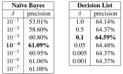
To increase the accuracy of our system, we needed to optimize various parameters by running the training data through 10-way cross-validation and averaging the scores from each set. Table 2 shows the results of this cross-validation in determining theδvalue used in the additive smoothing for both the Na¨ıve Bayes classifier and for the decision list classifier.

We also experimented with different feature sets. The results of these experiments are shown in Ta-ble 3.

Classifier Cross-Validation Score

MFS 34.99%

LSA 38.61%

k-NN Cosine 61.54% Na¨ıve Bayes 58.60% Decision List 64.37%

NN Cosine 65.56%

Simple Combined 65.89% Weighted Combined 67.38%

Classifier Competition Score

SWAT-MP 65.78%

Table 1: The (micro-averaged) precision of each of our classifiers in cross-validation, plus the actual re-sults from our entry in SemEval-2007.

Na¨ıve Bayes δ precision 10−1 _53.01% 10−2 _58.60% 10−3 _60.80%

10−4 _61.09% 10−5 _60.95% 10−6 _61.06% 10−7 _61.08%

Decision List δ precision 1.0 64.14% 0.5 64.37% 0.1 64.59% 0.05 64.48% 0.005 64.37% 0.001 64.37%

Table 2: On cross-validated training data, system precision when using different smoothing parame-ters in the Na¨ıve Bayes and decision list classifiers.

2.5 Conclusion

We presented a supervised system that used simple

n-gram features and a combination of five different

classifiers. The methods used are applicable to any lexical sample task, and have been applied to lexical sample tasks in previous Senseval competitions.

3 Task 14

Na¨ıve Bayes Feature Dec. List 55.36% word trigrams 59.98% 55.55% word bigrams 59.98% 58.50% weighted unigrams 62.77% 58.60% all features 64.37%

NN-Cosine Feature Combined 60.39% word trigrams 62.03% 60.42% word bigrams 62.66% 65.56% weighted unigrams 64.56% 62.92% all features 67.38%

Table 3: On cross-validated training data, the preci-sion when using different features with each classi-fier, and with the combination of all classifiers. All feature sets include a simple, unweighted bag-of-words in addition to the feature listed.

3.1 Training Data Collection

Our system is trained on a set of pre-annotated head-lines, building up a knowledge-base of individual words and their emotional significance.

We were initially provided with a trial-set of 250 annotated headlines. We ran 5-way cross-validation with a preliminary version of our system, and found that a dataset of that size was too sparse to effec-tively tag new headlines. In order to generate a more meaningful knowledge-base, we created a sim-ple web interface for human annotation of headlines. We used untrained, non-experts to annotate an addi-tional 1,000 headlines for use as a training set. The headlines were taken from a randomized collection of headlines from the Associated Press.

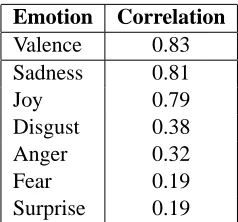
We included a subset of the original test set in the set that we put online so that we could get a rough estimate of the consistency of human annota-tion. We found that consistency varied greatly across the emotions. As can be seen in Table 4, our tors were very consistent with the trial data annota-tors on some emotions, while inconsistent on others. In ad-hoc, post-annotation interviews, our anno-tators commented that the task was very difficult. What we had initially expected to be a tedious but mindless exercise turned out to be rather involved. They also reported that some emotions were consis-tently harder to annotate than others. The results in Table 4 seem to bear this out as well.

Emotion Correlation Valence 0.83 Sadness 0.81

Joy 0.79

Disgust 0.38

Anger 0.32

Fear 0.19

Surprise 0.19

Table 4: Pearson correlations between trial data an-notators and our human anan-notators.

One difficulty reported by our annotators was de-termining whether to label the emotion experienced by the reader or by the subject of the headline. For example, the headline “White House surprised at reaction to attorney firings” clearly states that the White House was surprised, but the reader might not have been.

Another of the major difficulties in properly notating headlines is that many headlines can be an-notated in vastly different ways depending on the viewpoint of the annotator. For example, while the headline “Hundreds killed in earthquake” would be universally accepted as negative, the headline “Italy defeats France in World Cup Final,” can be seen as positive, negative, or even neutral depending on the viewpoint of the reader. These types of problems made it very difficult for our annotators to provide consistent labels.

3.2 Data Processing

Before we can process a headline and determine its emotions and valence, we convert our list of tagged headlines into a useful knowledge base. To this end, we create a word-emotion mapping.

3.2.1 Pre-processing

The first step is to lemmatize every word in every headline, in an attempt to reduce the sparseness of our data. We use the CELEX2 (Baayen et al., 1996) data to perform this lemmatization. There are unfor-tunate cases where lemmatizing actually changes the emotional content of a word (unfortunate becomes

fortunate), but without lemmatization, our data is

emo-tions and valence of every headline, H, in which that word, w, appears, ignoring non-content words:

Score(Em, w) = X

H:_{w ǫ H}

Score(Em, H)

In the final step of pre-processing, we add the synonyms and antonyms of the sense labels them-selves to our word-emotion mapping. We queried the web interface for Roget’s New Millennium The-saurus (TheThe-saurus.com, 2007) and added every word in the first 8 entries for each sense label to our map, with a score of100 (the maximum possible score) for that sense. We also added every word in the first 4 antonym entries with a score of−40. For exam-ple, for the emotion Joy, we added alleviation and

amusement with a score of100, and we added

de-spair and misery with a score of−40.

3.2.2 Processing

After creating our word-emotion mapping, pre-dicting the emotions and valence of a given headline is straightforward. We treat each headline as a bag-of-words and lemmatize each word. Then we look up each word in the headline in our word-emotion map, and average the emotion and valence scores of each word in our map that occurs in the headline. We ignore words that were not present in the train-ing data.

3.3 Evaluation

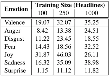
Emotion Training Size (Headlines) 100 250 1000 Valence 19.07 32.07 35.25 Anger 8.42 13.38 24.51 Disgust 11.22 23.45 18.55 Fear 14.43 18.56 32.52 Joy 31.87 46.03 26.11 Sadness 16.32 35.09 38.98 Surprise 1.15 11.12 11.82

Table 5: A comparison of results on the provided trial data as headlines are added to the training set. The scores are given as Pearson correlations of scores for training sets of size 100, 250, and 1000 headlines.

As can be seen in Table 5, four out of six emotions and the valence increase along with training set size.

This leads us to believe that further increases in the size of the training set would continue to improve results. Lack of time prevents a full analysis that can explain the sudden drop of Disgust and Joy.

Table 6 shows our full results from this task. Our system finished third out of five in the valence sub-task and second out of three in the emotion sub-sub-task.

Emotion Fine Coarse-Grained

A P R

Valence 35.25 53.20 45.71 3.42 Anger 24.51 92.10 12.00 5.00 Disgust 18.55 97.20 0.00 0.00 Fear 32.52 84.80 25.00 14.40 Joy 26.11 80.60 35.41 9.44 Sadness 38.98 87.70 32.50 11.92 Surprise 11.82 89.10 11.86 10.93

Table 6: Our full results from SemEval-2007, Task 14, as reported by the task organizers. Fine-grained scores are given as Pearson correlations. Coarse-grained scores are given as accuracy (A), preci-sion (P), and recall (R).

3.4 Conclusion

We presented a supervised system that used a un-igram model to annotate the emotional content of headlines. We also used synonym expansion on the emotion label words. Our annotators encountered significant difficulty while tagging training data, due to ambiguity in definition of the task.

References

R.H. Baayen, R. Piepenbrock, and L. Gulikers. 1996. CELEX2. LDC96L14, Linguistic Data Consortium, Philadelphia.

S. F. Chen and J. Goodman. 1998. An empirical study of smoothing techniques for language modeling. Techni-cal Report TR-10-98, Harvard University.

T.K. Landauer, Foltz P.W, and D. Laham. 1998. Intro-duction to latent semantic analysis. Discourse

Pro-cesses, 25:259–284.

Thesaurus.com. 2007. Roget’s New Millennium The-saurus, 1st ed. (v 1.3.1). Lexico Publishing Group,

Richard Wicentowski, Emily Thomforde, and Adrian Packel. 2004. The Swarthmore College

SENSEVAL-3System. In Proceedings of Senseval-3,

Third International Workshop on Evaluating Word Sense Disambiguation Systems.

David Yarowsky. 1994. Decision lists for lexical am-biguity resolution: Application to accent restoration in Spanish and French. In Proceedings of the 32nd