Fine grained domain classification of text using TERMIUM Plus

Fine-grained domain classification of text using TERMIUM Plus

Gabriel Bernier-Colborne, Caroline Barri`ere, Pierre Andr´e M´enard Centre de recherche informatique de Montr´eal

[email protected], [email protected], [email protected]

Abstract

In this article, we present the use of a term bank for text classification purposes. We developed a supervised text classification approach which takes advantage of the domain-based structure of a term bank, namely TERMIUM Plus, as well as its bilingual content. The goal of the text classification task is to correctly identify the appropriate fine-grained domains of short segments of text in both French and English. We developed a vector space model for this task, which we refer to as the DCVSM (domain classification vector space model). In order to train and evaluate the DCVSM, we generated two new datasets from the open data contained in TERMIUM Plus. Results on these datasets show that the DCVSM compares favourably to five other supervised classification algorithms tested, achieving the highest micro-averaged recall (R@1).

1

Introduction

Text classification is a well-known task in Natural Language Processing, which aims at automatically providing additional document-level metadata (e.g. domain, genre, author). To our knowledge, the curated domain structures found in term banks have never been used to automatically provide metadata describing the fine-grained domains discussed in a given document. This might perhaps be due to the fact that term banks have not been made available as open and free resources until recently, as well as the lack of text data annotated using a term bank’s domains as target classes, which is necessary for a supervised classification approach.

Our research was stimulated by the gap mentioned above, and our contribution, highlighted in this paper, is both to provide annotated datasets for fine-grained domain classification of texts, and a classi-fication method that achieves high accuracy. We should say that our first contribution is only possible because of the recent release of the term bank TERMIUM Plus, which contains both the domain struc-turing information and the short text segments which we use to build our two datasets, one for French and one for English. Our second contribution is a comparison of six different supervised classification algorithms on these datasets, which aims to determine which kind of classifier produces the best results on this task. Among the models we tested, the one which achieves the highest accuracy is a vector space model we developed for this task, which we refer to as the domain classification vector space model (DCVSM).

The datasets are described in Section 2 and the DCVSM is explained in Section 3. The experimental setup and results are presented in Sections 4 and 5. Related work is outlined in Section 6.

2

Datasets generated from Termium

The datasets we created for this research were extracted from TERMIUM PlusR_{, which we will call}

simplyTermiumfrom now on. Termium1is a multilingual terminology and linguistic data bank, devel-oped by the Translation Bureau of Canada for over thirty years, but only recently released as open data by the Government of Canada. Since 2014, an open version of Termium Plus is available, with periodic

1

updates. So far, it has not been used much for research on computational linguistics, yet it is a rich resource which can be used for such research in various ways, as we will show.

The latest release of Termium contains data in four languages: English, French, Castilian Spanish, and Portuguese. The datasets presented in this paper were extracted from a 2016 release of Termium, which only included English and French data. The release we used contains about 1.33 million records associated with 2252 domains. An example of a record is shown in Table 1.

English French

Terms 1.penalty kick; 2.penalty 1.coup de pied de r´eparation; 2.coup de pied de p´enalit´e; 3.coup de r´eparation; 4.coup de pied de punition; 5. tir de r´eparation; 6. tir de punition; 7.penalty; 8.penalty kick Definitions A kick, unopposed except for the goalkeeper,

awarded to sanction a foul committed by a de-fensive player in his own penalty area.

Coup tir´e sans opposition de l’adversaire pour sanctionner une faute commise par un joueur d´efensif dans sa propre surface de r´eparation.

Contexts The referee may award a penalty kick for an infringement of the laws.

Les coups de pied de p´enalit´e et les coups de pied francs sont accord´es `a l’´equipe non fau-tive `a la suite de fautes de [ses] adversaires.

Domains 1. Specialized Vocabulary and Phraseologism of Sports; 2. Soccer (Europe: Football); 3. Rugby

1. Vocabulaire sp´ecialis´e et phras´eologie des sports; 2. Soccer (Europe : football); 3. Rugby

Table 1: Excerpt from a record in Termium.

To create the datasets used in this research, we first had to process the source files containing the open data of Termium in order to reconstruct its records. The source files are organized by domain, and records belonging to multiple domains are represented by multiple rows, often in different files. Furthermore, the source files do not (currently) indicate which rows belong to the same record (i.e. using some kind of unique record identifier). Therefore, data fusion must be performed to reconstruct the records. The principle used to perform the data fusion is that rows that belong to the same record are identical except for the domain fields. By merging the rows which are identical except for these fields and combining the values found in these fields, we can reconstruct Termium’s records. Note that there are exceptions to this rule which produce a small quantity of noise (i.e. mismatches between the records shown in the web version of Termium and the index we created using the source files). Thus the 2 million rows in the source files were aggregated into 1.33 million indexed records, from which we extracted the datasets described below. We have released this data2in order to make it easier to reproduce the results reported in this paper, and more generally, to train a classifier using the fine-grained classification of Termium.

As illustrated in Table 1, records in Termium are all linked to at least one domain, and many are linked to 2 domains (31% of records), 3 domains (8%) or more (1%). Records can also contain various kinds of textual supports such as a definition or examples which illustrate the use of a term, known ascontexts. Termium contains about 170 000 of these contexts in English and 155 000 in French, not counting duplicates. These contexts are meant to illustrate the use of a term, but they sometimes also contain definitional or encyclopedic information about the term. Unlike definitions, which often do not contain the term they define, contexts usually contain an occurrence of one of the synonymous terms on the record, as they are meant to illustrate usage. We created two gold standard datasets by extracting these contexts and their associated domains from Termium, one in English and one in French. We will refer to them as the Termium Context (TC) datasets.

Although the contexts in Termium are supposed to show terms in use, we found out during our experiments that some records contain a context in which none of the record’s terms actually occur. Therefore, we defined a procedure to automatically validate each context by checking if it contained at least one of the terms of the record(s) in which it was found. The contexts shown in Table 1 are examples of valid contexts as they contain the termspenalty kickandcoup de pied de p´enalit´e. About 85% of the

Context Domain

The use ofJacobson’s organis most obvious in snakes. If a strong odour or vibration stimulates a snake, its tongue is flicked in and out rapidly. Each time it is retracted the forked tip touches the opening ofJacobson’s organin the roof of the mouth, transmitting any chemical fragments adhering to the tongue.

Reptiles and Amphibians

The rate of speed of a composition or a section thereof, ranging from the slowest to the quickest, as is indicated bytempomarks such as largo, adagio, andante, moderato, allegro, presto, prestissimo ...

Musicology

A player is “onside” when either of his skates are in physical contact with or on his own side of the line at the instant the puck completely crosses the outer edge of that line regardless of the position of his stick.

Ice Hockey

Table 2: Examples of labeled contexts included in the datasets. Terms in bold are those illustrated by each context.

contexts in each language passed this test.

Some contexts appear on multiple records and are associated with several domains, but most are associated with one or two domains, which are often related by a hierarchical relationship (e.g. Zoology andReptiles and Amphibians). We decided to treat the classification task as a single-label classification task, therefore only one domain label was retained for each context. This makes the task more difficult, as only one domain is considered correct when evaluating the predictions of a classifier for a given context, even if that context belongs to multiple, related domains according to Termium. To select a single label for these contexts, we used a frequency-based heuristic which favours less frequent (and perhaps more specific) domains. Subsequently, a minimum class (domain) frequency of 20 was imposed, which removed about 5% of the remaining contexts in each language.

English French

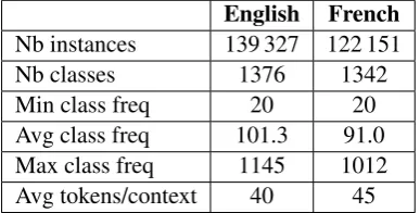
Nb instances 139 327 122 151

Nb classes 1376 1342

Min class freq 20 20 Avg class freq 101.3 91.0 Max class freq 1145 1012 Avg tokens/context 40 45

Table 3: TC Datasets statistics. Each instance in the TC datasets comprises a context

and a domain label, as shown in Table 2. Statistics on the TC datasets are presented in Table 3. Contexts contain about 40-45 tokens on average, which makes these texts much shorter than those typically used to evaluate text classification, yet longer than a typical query in informa-tion retrieval. The number of classes (1376 in English, 1342 in French) is also higher than that of other text clas-sification datasets, such as Reuters-215783, which con-tains 118 classes. Thus, this task can be considered a fine-grained domain classification of short texts.

3

Domain Classification Vector Space Model

The domain classification vector space model (DCVSM) we developed follows the general principles of vector space models4. To predict the domain of a short text, the DCVSM considers the short text as a query and Termium domains as pseudo-documents. The underlying principle is that a Termium domain can be viewed as a document containing all the contexts found in the term bank’s records and associated with that domain. The short text can then be classified by computing its similarity to each domain (or pseudo-document). We formally define the DCVSM below as a supervised classifier, and compare it to other classifiers in the following sections.

LetC ={c1, . . . , cm}be the set of classes andF ={f1, . . . , fn}the set of features. A supervised classifier is trained using a collectionXof labelled feature vectorshx, ci, wherex ∈ _Rn _{is the feature} vector and cis its class. To train the DCVSM, we calculate a matrixW which indicates for each pair

3

Seehttp://www.daviddlewis.com/resources/testcollections/reuters21578/readme.txt.

4

(fi,cj) the strength of the association between featurefi and classcj. In the case of the text classifica-tion task addressed in this paper, the features are words and the classes are domains, so each valueWij represents the importance of wordfi in domain cj. Thus, matrix W is similar to the word-document matrices commonly used for text classification and information retrieval (Salton, 1971), word similar-ity estimation (Turney and Pantel, 2010), and related tasks. These matrices are typically calculated by counting how many times each word occurs in each document, then weighting these frequencies us-ing a scheme such as tf-idf (Sp¨arck Jones, 1972) or an association measure such as pointwise mutual information (Church and Hanks, 1989).

MatrixW is calculated using the following method. For each pair (fi, cj), we sum up the values of featurefi for each feature vector in the training data that belongs to classcj, which we will noteTficj. This can be formulated as follows: Tficj =Phx,ci∈X_cjxi. whereXcj is the subset of training instances belonging to classcj, andxiis the value of featurefiinx(e.g. the weighted frequency of a word). This sum is then weighted to estimate the association between the feature and the class: Wij = ψ(Tficj), whereψis some weighting function. The resulting valueWij is the weight of featurefifor classcj.

Each column vectorW:j represents the feature weights of the classifier for classcj. A new feature vector x is classified by calculating the dot product of x and the feature weights of each class, and selecting the class which maximises this function. In other words,W:j represents a pseudo-document corresponding to domaincj, and contexts are classified by finding the most similar pseudo-document. Formally, the probability of a classcj is defined as follows: Pr(cj|x)∝Pn_i=1xiWij.

The DCVSM assumes that the contribution of each feature to the likelihood of a class is independent of the other features. Many other classifiers make this assumption, including the multinomial Naive Bayes classifier which is often used for text classification. Furthermore, like Naive Bayes, the DCVSM is fast, scalable, and simple to train, as training only involves calculating matrixW on the training data. Naive Bayes is one of the five classifiers to which we compare the DCVSM in the following experiment.

4

Text classification experiment

Using the TC datasets (in English and French) described in Section 2, we evaluated the DCVSM as well as five other supervised classification algorithms that have been used for text classification. Each short text (instance) from a TC dataset was converted into a bag of words after applying basic preprocessing (tokenization, lemmatization, case-folding, and removal of stop words and punctuation)5_{. Thus, each}

instance is represented by a feature vector where each value is the frequency of a specific word. The set of features contains every word that occurs at least twice in the training data. Word frequencies were optionally weighted using tf-idf, with idf being defined as follows for a given wordw: idf(w) =

log

_|

D| |Dw|+ 1

, whereDis the set of contexts used for training,|D|is its size, andDw is the subset of training contexts that containw.

The five other supervised classification algorithms we tested are: multinomial Naive Bayes (NB), Rocchio classification (RC), softmax regression (SR), k-nearest neighbours (k-NN) and a multi-layer perceptron (MLP).

As noted above, multinomial Naive Bayes is commonly used for text classification. Rocchio classifi-cation (Rocchio, 1971), like Naive Bayes, is a linear classificlassifi-cation algorithm. The DCVSM is similar to Rocchio classification, which involves computing centroids by averaging all the feature vectors belong-ing to each class, and classifybelong-ing new instances by assignbelong-ing them to the class of the nearest centroid. The DCVSM is different in that the feature vectors belonging to each class are summed rather than being averaged, and then weighted.

Softmax regression (or multinomial logistic regression) is also a linear classification algorithm. The softmax classifier was trained using stochastic gradient descent, with a penalty on the L2 norm of the feature weights for regularisation.

5_{Stanford’s CoreNLP library (Manning et al., 2014) was used for tokenization. TreeTagger (Schmid, 1994) and TT4J}

The k-NN algorithm and the MLP are non-linear classifiers. k-NN classifies a given instance based on the classes of the kmost similar instances in the training data. The MLP is also known as a fully connected artificial neural network. A description of artificial neural networks and the backpropagation algorithm used to train them can be found in Rumelhart et al. (1986), and Bengio (2012) provides a practical guide to training and tuning neural networks. We tested MLPs containing 1 or 2 hidden layers of exponential linear units (Clevert et al., 2015). The MLP was trained using the Adam algorithm (Kingma and Ba, 2014) and regularised using dropout and a max-norm constraint on the incoming weights of all units (Srivastava et al., 2014).

Each TC dataset was split into 3 subsets of equal size (about 46K instances in English and 41K in French) for training, validation, and testing. A grid search was used to tune the hyperparameters of each classifier on the validation set (except Naive Bayes, which has no hyperparameters). Then the best configuration of each classifier was evaluated on the held-out test set. Each classifier was tuned and tested twice, once using raw word frequencies as input, and once using tf-idf weighted frequencies. The impact of this weighting will be assessed in the next section.

For the DCVSM, the only hyperparameter is the weighting schemeψ used to compute the feature weights. We tested nine different weighting schemes including tf-idf6_{and the simple association}

mea-sures defined in Evert (2007, ch. 4). These association meamea-sures compare the observed frequency of (word, context) pairs to their expected frequency in order to measure the strength of their association. We calculate this expectation using the following equation:

E[Tficj] =

Pm

j0₌₁Tfic_j0 Pn

i0₌₁Tf_i0cj Pn

i0₌₁Pm_j0₌₁T_f

i0cj0

where Tficj, as defined earlier (see Section 3), is the sum, for each feature vector in the training data belonging to class cj, of the value of feature fi. We set all of the association measures to 0 if

Tficj <= E[Tficj]. We optionally apply a log or square root transformation to the output of all the weighting schemes, following Lapesa et al. (2014).

For Rocchio classification, we tuned the measure used to estimate the distance between a feature vec-tor and the class centroids (euclidean distance or cosine). For k-NN, we tuned the number of neighbours (k) and the distance-based weighting of neighbours. For the softmax classifier, we tuned the learning rate and the L2 penalty coefficient. As for the MLP, we tuned the number of hidden layers (1 or 2), the number of units in each, the learning rate, the number of training iterations (epochs), the dropout probability and the max-norm constraint.

5

Results

Table 4 shows the accuracy achieved by each classifier on the test sets in English and French. Accuracy is measured using two different evaluation measures, namely micro-averaged recall at rank 1 (R@1) and recall at rank 5 (R@5). R@1 is simply the percentage of correctly classified instances. This is the measure that was used to tune the models on the validation set. It only considers the top prediction of a classifier for a given test case, whereas R@5 considers the top five predictions. In other words, R@5 is the percentage of test cases for which the correct class is among the five most likely classes according to the classifier.

The results indicate that the DCVSM achieves a higher R@1 than the five other classifiers tested, and the second-highest R@5, just behind the MLP. The DCVSM does not fit the training data as well as other classifiers, yet it achieves the highest R@1 on the held-out data used for testing. The MLP can easily fit the training data perfectly (as can k-NN), which the DCVSM cannot. Regularisation techniques (dropout, max-norm constraint, early stopping) were used to avoid overfitting the training data using the MLP, yet no configuration we tested scored better on the validation data (in terms of R@1) than

6

R@1 R@5

EN FR EN FR

k-NN 0.104 0.080 0.107 0.085 NB 0.224 0.218 0.442 0.430 SR 0.245 0.241 0.494 0.476 RC 0.253 0.253 0.504 0.498 MLP 0.264 0.260 0.530 0.521

DCVSM 0.283 0.277 0.529 0.512

Table 4: Micro-averaged R@1 and R@5 on the test sets in English and French.

∆R@1 ∆R@5

EN FR EN FR

k-NN -0.016 +0.005 -0.016 +0.005 NB +0.051 +0.072 +0.085 +0.140 SR +0.016 +0.020 +0.034 +0.042 RC +0.066 +0.108 +0.122 +0.198 MLP -0.005 -0.002 -0.006 -0.005 DCVSM -0.008 -0.002 -0.007 -0.001

Table 5: Impact of weighting the feature values us-ing tf-idf.

the DCVSM. It remains possible that higher accuracy could be achieved using an MLP by testing other regularisation or optimisation techniques. It is also possible that the DCVSM could produce even higher accuracy if we tested other weighting schemes.

The scores shown in Table 4 represent the best of two scores for each classifier, using either raw word frequencies or tf-idf weighted frequencies as input. Table 5 shows the impact of using tf-idf to weight the word frequencies on the accuracy achieved by each classifier on the test sets. These results show that the DCVSM performs slightly better when feature values are raw word frequencies, as does the MLP. Other classifiers perform much worse when the input is not weighted using tf-idf, especially the Naive Bayes and Rocchio classifiers.

To gain insight on both the datasets and the DCVSM, we inspected the classes on which the DCVSM achieved the lowest and highest recall. The classes for which recall was highest on the test set in English are shown in Table 6, along with the top features for each of these classes, most of which do seem like good predictors for these classes.

Class R@1 Top features

Solid Fuel Heating 1.000 stoker, grate, chain-grate, stokers, traveling-grate, underfeed, pul-verize, pulverizer, direct-fired, coal, . . .

Opening and Closing Devices (Packaging)

0.900 press-on, closure, dauber, innerseal, cap, foil, applicator, ct, heat-sealed, hermetic, . . .

Hats and Millinery 0.900 hat, brim, bicorne, chinstrap, milliner, tricorne, courtier, gentle-man, cock, napoleon, . . .

Tunnels Overpasses and Bridges

0.880 bridge, span, anchorage, abutment, pontoon, girder, cantilever, pier, 700-m, bridges, . . .

Electoral Systems and Political Parties

0.875 election, ballot, electoral, elector, voting, polling, vote, voter, can-didate, officer, . . .

Deep Foundations 0.867 pile, caisson, pier, hammer, excavation, fuel-injection, morris, concrete, piling, pinning, . . .

Yoga and Pilates 0.864 yoga, chakra, bandha, muladhara, pranayama, vinyasa, pose, bhedana, chakras, meditation, . . .

Table 6: High-recall classes and their top features.

Predicted class Correct class

Radio Transmission and Reception [54] Radio Interference [10] Criminology [61] Criminal Psychology [14] Advertising [46] Advertising Techniques [31] Human Behaviour [55] Animal Behaviour [48] Artificial Intelligence [383] Philosophy (General) [21]

Table 7: Low-recall classes (right) and the classes with which they are most often confused (left). The frequency of each class is shown in brackets. This is their frequency in the training set (in English).

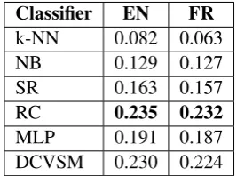
Classifier EN FR

k-NN 0.082 0.063 NB 0.129 0.127 SR 0.163 0.157 RC 0.235 0.232

MLP 0.191 0.187 DCVSM 0.230 0.224

Table 8: Macro-averaged R@1. An analysis of class-wise recall with respect to class

fre-quency confirmed that recall is systematically lower on low-frequency classes. If we compare the classifiers using macro-averaged (rather than micro-macro-averaged) R@1, i.e. the average R@1 per class across all classes, we obtain the results shown in Table 8. The DCVSM performs better in this respect than every other algorithm except Rocchio classification. It is im-portant to remember that the models were tuned by optimiz-ing micro-averaged R@1, and that optimizoptimiz-ing macro-averaged R@1 would produce different results.

6

Related Work

We have outlined similarities between the DCVSM presented in this paper and other classification al-gorithms in section 3. It is worth noting that the DCVSM is related to methods such as explicit se-mantic analysis or ESA (Gabrilovich and Markovitch, 2007). In ESA, texts are represented in a high-dimensional space of explicit concepts or categories, based on associations between words and these categories. These associations are calculated on some knowledge base, typically Wikipedia, using tf-idf. The main difference between this and the DCVSM presented in this paper is that ESA computes feature weights (i.e. word-category associations) using category-labeled Wikipedia articles as training data.

Mohammad and Hirst (2006) compute associations between words and categories for disambiguation purposes, which are similar to the word-domain associations discussed in this paper. Mohammad and Hirst (2006) calculate these associations using unlabelled text and a thesaurus, whereas we use labeled text, which renders the bootstrapping procedure they propose unnecessary, as the relevant domains of each text are known.

Also worth mentioning is the text classification algorithm introduced by Navigli et al. (2011), which exploits the structure of WordNet (Fellbaum, 1998) and is used to identify the domain of a document. This is evaluated on a (single label) dataset of domain-labelled Wikipedia articles. For reference, they obtain a micro-averaged R@1 of 0.670, which is more than twice as high as the maximum obtained on the task tackled in this paper. However, the articles in their dataset are much longer than the contexts in Termium, the number of domains (29) is smaller by two orders of magnitude, and the prior probabilities of the domains are uniform. The fine-grained nature of the domain classification presented in this paper makes the task more difficult, as does the short length of the texts.

7

Concluding remarks and future work

the DCVSM performed well, achieving the highest micro-averaged recall (R@1) and the second-highest macro-averaged recall.

Future work will focus on applications of the DCVSM and the TC datasets. In particular, we wish to go back to the work described in Barri`ere et al. (2016) and further evaluate the DCVSM on a disambigua-tion task. The fact that the DCVSM can identify the domain of a short text with relatively high accuracy, as shown in this paper, can be useful in itself, but this information can also be used to disambiguate the words or terms that appear in the text. Domain-driven disambiguation methods first identify the relevant domains of the context in which an ambiguous term (or word) occurs, then use this domain information to identify the sense conveyed by that term in that context. Some methods based on domain identification have been used for word sense disambiguation in Magnini et al. (2001); Gliozzo et al. (2005); Navigli et al. (2011). In our own previous work (Barri`ere et al., 2016), we performed domain-driven term sense disambiguation, but the disambiguation algorithm exploited a different text classifier. In future work, we plan on measuring the impact of using the higher-accuracy text classifier presented here within our term disambiguation algorithm.

In a more general perspective, we could investigate how representing texts using the fine-grained domain classification of Termium would impact performance on other tasks. Classifying a text using this classification produces a score for each domain, indicating the likelihood that the text is related to that domain. This list of scores can be considered a representation of the text in a high-dimensional space of domains. Representing texts in this domain space could be useful for other classification or clustering purposes, with different applications in mind. We hope our research will help promote the use of terminological resources for such diverse NLP applications. With this in mind, we have made the datasets we developed available to the research community.

Acknowledgments

This research was carried out as part of the PACTE project (M´enard and Barri`ere, 2017), and was sup-ported by CANARIE and theminist`ere de l’ ´Econonomie, de la Science et de l’Innovation(MESI) of the Government of Qu´ebec.

References

Barri`ere, C., P. A. M´enard, and D. Azoulay (2016). Contextual term equivalent search using domain-driven disambiguation. InProceedings of the 5th International Workshop on Computational Termi-nology (CompuTerm 2016), pp. 21–29.

Bengio, Y. (2012). Practical recommendations for gradient-based training of deep architectures. CoRR abs/1206.5533.

Church, K. W. and P. Hanks (1989). Word association norms, mutual information, and lexicography. In Proceedings of the 27th Annual Meeting of the Association for Computational Linguistics, pp. 76–83.

Clevert, D., T. Unterthiner, and S. Hochreiter (2015). Fast and accurate deep network learning by expo-nential linear units (elus). CoRR abs/1511.07289.

Evert, S. (2007). Corpora and collocations (extended manuscript). In A. L¨udeling and M. Kyt¨o (Eds.), Corpus Linguistics. An International Handbook, Volume 2. Berlin/New York: Walter de Gruyter.

Fellbaum, C. (1998). WordNet: An Electronic Lexical Database. Bradford Books.

Gliozzo, A., C. Giuliano, and C. Strapparava (2005). Domain kernels for word sense disambiguation. In Proceedings of the 43rd Annual Meeting of the Association for Computational Linguistics (ACL), pp. 403–410. ACL.

Kingma, D. P. and J. Ba (2014). Adam: A method for stochastic optimization. CoRR abs/1412.6980.

Lapesa, G., S. Evert, and S. Schulte im Walde (2014). Contrasting syntagmatic and paradigmatic rela-tions: Insights from distributional semantic models. InProceedings of the Third Joint Conference on Lexical and Computational Semantics (*SEM 2014), pp. 160–170. ACL/DCU.

Magnini, B., C. Strapparava, G. Pezzulo, and A. Gliozzo (2001). Using domain information for word sense disambiguation. In Proceedings of the Second International Workshop on Evaluating Word Sense Disambiguation Systems, pp. 111–114. ACL.

Manning, C. D., P. Raghavan, and H. Sch¨utze (2009). Introduction to Information Retrieval (online edition). Cambridge University Press.

Manning, C. D., M. Surdeanu, J. Bauer, J. Finkel, S. J. Bethard, and D. McClosky (2014). The Stanford CoreNLP natural language processing toolkit. InProceedings of the 52nd Annual Meeting of the Association for Computational Linguistics (ACL): System Demonstrations, pp. 55–60.

Mohammad, S. and G. Hirst (2006). Determining word sense dominance using a thesaurus. In Pro-ceedings of the Eleventh Conference of the European Chapter of the Association for Computational Linguistics (EACL), pp. 121–128. ACL.

M´enard, P. A. and C. Barri`ere (2017). PACTE: A collaborative platform for textual annotation. In13th Joint ISO-ACL Workshop on Interoperable Semantic Annotation (ISA-13).

Navigli, R., S. Faralli, A. Soroa, O. de Lacalle, and E. Agirre (2011). Two birds with one stone: learning semantic models for text categorization and word sense disambiguation. InProceedings of the 20th ACM International Conference on Information and Knowledge Management, pp. 2317–2320. ACM.

Rocchio, J. J. (1971). Relevance feedback in information retrieval. See Salton (1971).

Rumelhart, D. E., G. E. Hinton, and R. J. Williams (1986). Learning representations by back-propagating errors. Nature 323, 533–536.

Salton, G. (Ed.) (1971).The SMART Retrieval System – Experiments in Automatic Document Processing. Prentice Hall.

Schmid, H. (1994). Probabilistic part-of-speech tagging using decision trees. In Proceedings of the International Conference on New Methods in Language Processing.

Sp¨arck Jones, K. (1972). A statistical interpretation of term specificity and its application in retrieval. Journal of documentation 28(1), 11–21.

Srivastava, N., G. E. Hinton, A. Krizhevsky, I. Sutskever, and R. Salakhutdinov (2014). Dropout: a simple way to prevent neural networks from overfitting.Journal of Machine Learning Research 15(1), 1929–1958.