A Simple, Fast, and Effective Reparameterization of IBM Model 2

A Simple, Fast, and Effective Reparameterization of IBM Model 2

Chris Dyer Victor Chahuneau Noah A. Smith Language Technologies Institute

Carnegie Mellon University Pittsburgh, PA 15213, USA

{cdyer,vchahune,nasmith}@cs.cmu.edu

Abstract

We present a simple log-linear reparame-terization of IBM Model 2 that overcomes problems arising from Model 1’s strong assumptions and Model 2’s overparame-terization. Efficient inference, likelihood evaluation, and parameter estimation algo-rithms are provided. Training the model is consistently ten times faster than Model 4. On three large-scale translation tasks, systems built using our alignment model outperform IBM Model 4.

An open-source implementation of the align-ment model described in this paper is available fromhttp://github.com/clab/fast align.

1 Introduction

Word alignment is a fundamental problem in statis-tical machine translation. While the search for more sophisticated models that provide more nuanced ex-planations of parallel corpora is a key research activ-ity, simple and effective models that scale well are also important. These play a crucial role in many scenarios such as parallel data mining and rapid large scale experimentation, and as subcomponents of other models or training and inference algorithms. For these reasons, IBM Models 1 and 2, which sup-port exact inference in timeΘ(|f| · |e|), continue to be widely used.

This paper argues that both of these models are suboptimal, even in the space of models that per-mit such computationally cheap inference. Model 1 assumes all alignment structures are uniformly

likely (a problematic assumption, particularly for frequent word types), and Model 2 is vastly overpa-rameterized, making it prone to degenerate behav-ior on account of overfitting.1 We present a simple log-linear reparameterization of Model 2 that avoids both problems (_§2). While inference in log-linear models is generally computationally more expen-sive than in their multinomial counterparts, we show how the quantities needed for alignment inference, likelihood evaluation, and parameter estimation us-ing EM and related methods can be computed usus-ing two simple algebraic identities (_§3), thereby defus-ing this objection. We provide results showdefus-ing our model is an order of magnitude faster to train than Model 4, that it requires no staged initialization, and that it produces alignments that lead to significantly better translation quality on downstream translation tasks (_§4).

2 Model

Our model is a variation of the lexical translation models proposed by Brown et al. (1993). Lexical translation works as follows. Given a source sen-tence f with length n, first generate the length of the target sentence,m. Next, generate analignment,

a = ha1, a2, . . . , ami, that indicates which source word (or null token) each target word will be a trans-lation of. Last, generate themoutput words, where eachei depends only onfai.

The model of alignment configurations we pro-pose is a log-linear reparameterization of Model 2.

1

Model 2 has independent parameters for every alignment position, conditioned on the source length, target length, and current target index.

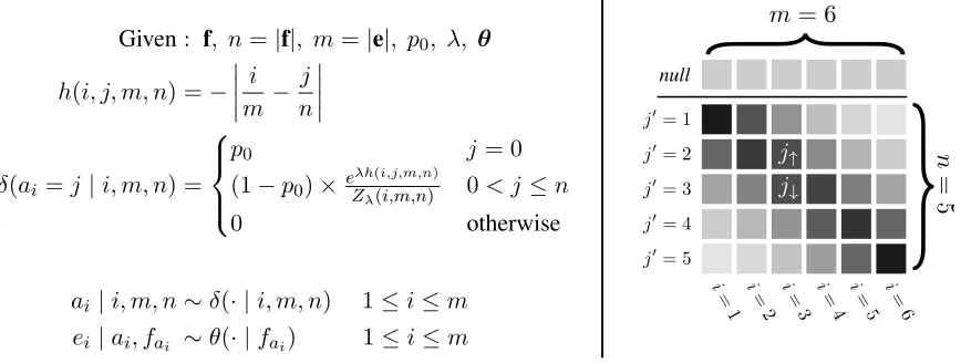
Given: f, n=_|f_|, m=_|e_|, p0, λ, θ

h(i, j, m, n) =−

i m −

j n

δ(ai=j|i, m, n) =     

p0 j= 0

(1₋p0)×e

λh(i,j,m,n)

Zλ(i,m,n) 0< j≤n

0 otherwise

ai|i, m, n∼δ(· |i, m, n) 1≤i≤m ei|ai, fai ∼θ(· |fai) 1≤i≤m

null

j�_{= 1}

j�= 2

j�_{= 3}

j�= 4

j�= 5

i₌

3

}

=5

}

m= 6

i₌

1

i₌

2

i₌

4

i₌

5

i₌

6

j_↓ j_↑

Figure 1: Our proposed generative process yielding a translationeand its alignmentato a source sentencef, given the source sentencef, alignment parametersp0andλ, and lexical translation probabilitiesθ(left); an example visualization of the distribution of alignment probability mass under this model (right).

Our formulation, which we write as δ(ai = j | i, m, n), is shown in Fig. 1.2 The distribution over alignments is parameterized by a null alignment probability p0 and a precision λ ≥ 0 which

con-trols how strongly the model favors alignment points close to the diagonal. In the limiting case asλ_→0, the distribution approaches that of Model 1, and, as it gets larger, the model is less and less likely to de-viate from a perfectly diagonal alignment. The right side of Fig. 1 shows a graphical illustration of the alignment distribution in which darker squares indi-cate higher probability.

3 Inference

We now discuss two inference problems and give ef-ficient techniques for solving them. First, given a sentence pair and parameters, compute the marginal likelihood and the marginal alignment probabilities. Second, given a corpus of training data, estimate likelihood maximizing model parameters using EM.

3.1 Marginals

Under our model, the marginal likelihood of a sen-tence pair _hf,e_i can be computed exactly in time

2

Vogel et al. (1996) hint at a similar reparameterization of Model 2; however, its likelihood and its gradient are not effi-cient to evaluate, making it impractical to train and use. Och and Ney (2003) likewise remark on the overparameterization issue, removing a single variable of the original conditioning context, which only slightly improves matters.

Θ(|f| · |e|). This can be seen as follows. For each position in the sentence being generated, i _∈

[1,2, . . . , m], the alignment to the source and its translation is independent of all other translation and alignment decisions. Thus, the probability that the ith word ofeiseican be computed as:

p(ei, ai |f, m, n) =δ(ai |i, m, n)×θ(ei|fai)

p(ei |f, m, n) = n X j=0

p(ei, ai=j|f, m, n).

We can also compute the posterior probability over alignments using the above probabilities,

p(ai|ei,f, m, n) =

p(ei, ai|f, m, n) p(ei |f, m, n)

. (1)

Finally, since all words in e (and their alignments) are conditionally independent,3

p(e_|f) =

m Y i=1

p(ei |f, m, n)

=

m Y i=1

n X j=0

δ(ai |i, m, n)×θ(ei|fai).

3

3.2 Efficient Partition Function Evaluation

Evaluating and maximizing the data likelihood un-der log-linear models can be computationally ex-pensive since this requires evaluation of normalizing partition functions. In our case,

Zλ(i, m, n) = n X j0₌₁

expλh(i, j0, m, n).

While computing this sum is obviously possible inΘ(_|f_|) operations, our formulation permits exact computation inΘ(1), meaning our model can be ap-plied even in applications where computational ef-ficiency is paramount (e.g., MCMC simulations). The key insight is that the partition function is the (partial) sum of two geometric series of unnormal-ized probabilities that extend up and down from the probability-maximizing diagonal. The closest point on or above the diagonalj↑, and the next point down

j↓(see the right side of Fig. 1 for an illustration), is

computed as follows:

j↑=

i_×n

m

, j↓ =j↑+ 1.

Starting at j↑ and moving up the alignment

col-umn, as well as starting atj↓ and moving down, the

unnormalized probabilities decrease by a factor of r= exp−_nλ per step.

To compute the value of the partition, we only need to evaluate the unnormalized probabilities at j↑andj↓and then use the following identity, which

gives the sum of the first`terms of a geometric se-ries (Courant and Robbins, 1996):

s`(g1, r) =

` X k=1

g1rk−1 =g1

1₋r`

1₋r .

Using this identity,Zλ(i, m, n)can be computed as

sj↑(eλh(i,j↑,m,n), r) +sn−j↓(eλh(i,j↓,m,n), r).

3.3 Parameter Optimization

To optimize the likelihood of a sample of parallel data under our model, one can use EM. In the E-step, the posterior probabilities over alignments are com-puted using Eq. 1. In the M-step, the lexical trans-lation probabilities are updated by aggregating these

as counts and normalizing (Brown et al., 1993). In the experiments reported in this paper, we make the further assumption that θf ∼ Dirichlet(µ) where µi = 0.01 and approximate the posterior distribu-tion over theθf’s using a mean-field approximation (Riley and Gildea, 2012).4

During the M-step, the λ parameter must also be updated to make the E-step posterior distribu-tion over alignment points maximally probable un-der δ(_{· |} i, m, n). This maximizing value cannot be computed analytically, but a gradient-based op-timization can be used, where the first derivative (here, for a single target word) is:

∇λL=Ep(ai|ei,f,m,n)[h(i, ai, m, n)]

−Eδ(j0_|i,m,n)h(i, j0, m, n) (2)

The first term in this expression (the expected value ofh under the E-step posterior) is fixed for the du-ration of each M-step, but the second term’s value (the derivative of the log-partition function) changes many times asλis optimized.

3.4 Efficient Gradient Evaluation

Fortunately, like the partition function, the deriva-tive of the log-partition function (i.e., the second term in Eq. 2) can be computed in constant time us-ing an algebraic identity. To derive this, we observe that the values of h(i, j0, m, n) form an arithmetic sequence about the diagonal, with common differ-enced = ₋1/n. Thus, the quantity we seek is the sum of a series whose elements are the products of terms from an arithmetic sequence and those of the geometric sequence above, divided by the partition function value. This construction is referred to as an arithmetico-geometric series, and its sum may be computed as follows (Fernandez et al., 2006):

t`(g1,a1, r, d) =

` X k=1

[a1+d(k−1)]g1rk−1

= a`g`+1−a1g1 1−r +

d(g`+1−g1r)

(1−r)2 .

In this expression r, the g1’s and the `’s have the

same values as above,d = −1/nand the a1’s are

4

equal to the value ofh evaluated at the starting in-dices,j↑andj↓; thus, the derivative we seek at each

optimization iteration inside the M-step is:

∇λL=Ep(ai|ei,f,m,n)[h(i, ai, m, n)]

− 1

Zλ

(tj↑(eλh(i,j↑,m,n), h(i, j↑, m, n), r, d)

+tn−j↓(eλh(i,j↓,m,n), h(i, j↑, m, n), r, d)).

4 Experiments

In this section we evaluate the performance of our proposed model empirically. Experiments are conducted on three datasets representing different language typologies and dataset sizes: the FBIS Chinese-English corpus (LDC2003E14); a French-English corpus consisting of version 7 of the Eu-roparl and news-commentary corpora;5 and a large Arabic-English corpus consisting of all parallel data made available for the NIST 2012 Open MT evalua-tion. Table 1 gives token counts.

We begin with several preliminary results. First, we quantify the benefit of using the geometric series trick (§3.2) for computing the partition function rel-ative to na¨ıve summation. Our method requires only

0.62seconds to compute all partition function values for0 < i, m, n <150, whereas the na¨ıve algorithm requires6.49seconds for the same.6

Second, using a10k sample of the French-English data set (only 0.5%of the corpus), we determined 1) whetherp0 should be optimized; 2) what the

op-timal Dirichlet parameters µi are; and 3) whether the commonly used “staged initialization” procedure (in which Model 1 parameters are used to initialize Model 2, etc.) is necessary for our model. First, like Och and Ney (2003) who explored this issue for training Model 3, we found that EM tended to find poor values forp0, producing alignments that were

overly sparse. By fixing the value at p0 = 0.08,

we obtained minimal AER. Second, like Riley and Gildea (2012), we found that small values ofα proved the alignment error rate, although the im-pact was not particularly strong over large ranges of

5_{http://www.statmt.org/wmt12} 6

While this computational effort is a small relative to the total cost in EM training, in algorithms whereλchanges more rapidly, for example in Bayesian posterior inference with Monte Carlo methods (Chahuneau et al., 2013), this savings can have substantial value.

Table 1: CPU time (hours) required to train alignment models in one direction.

Language Pair Tokens Model 4 Log-linear Chinese-English 17.6M 2.7 0.2

French-English 117M 17.2 1.7

Arabic-English 368M 63.2 6.0

Table 2: Alignment quality (AER) on the WMT 2012 French-English and FBIS Chinese-English. Rows with EM use expectation maximization to estimate theθf, and

∼Dir use variational Bayes.

Model Estimator FR-EN ZH-EN

Model 1 EM 29.0 56.2

Model 1 ∼Dir 26.6 53.6

Model 2 EM 21.4 53.3

Log-linear EM 18.5 46.5

Log-linear _∼Dir 16.6 44.1

Model 4 EM 10.4 45.8

Table 3: Translation quality (BLEU) as a function of alignment type.

Language Pair Model 4 Log-linear Chinese-English 34.1 34.7

French-English 27.4 27.7

Arabic-English 54.5 55.7

α. Finally, we (perhaps surprisingly) found that the standard staged initialization procedure wasless ef-fectivein terms ofAERthan simply initializing our

model with uniform translation probabilities and a small value of λand running EM. Based on these observations, we fixedp0 = 0.08, µi = 0.01, and set the initial value ofλto4 for the remaining ex-periments.7

We next compare the alignments produced by our model to the Giza++ implementation of the standard IBM models using the default training procedure and parameters reported in Och and Ney (2003). Our model is trained for5 iterations using the pro-cedure described above (_§3.3). The algorithms are

7

compared in terms of (1) time required for training; (2) alignment error rate (AER, lower is better);8 and (3) translation quality (BLEU, higher is better) of hi-erarchical phrase-based translation system that used the alignments (Chiang, 2007). Table 1 shows the CPU time in hours required for training (one direc-tion, English is generated). Our model is at least

10_× faster to train than Model 4. Table 3 reports the differences in BLEUon a held-out test set. Our model’s alignments lead to consistently better scores than Model 4’s do.9

5 Conclusion

We have presented a fast and effective reparameteri-zation of IBM Model 2 that is a compelling replace-ment for for the standard Model 4. Although the alignment quality results measured in terms ofAER

are mixed, the alignments were shown to work ex-ceptionally well in downstream translation systems on a variety of language pairs.

Acknowledgments

This work was sponsored by the U. S. Army Research Laboratory and the U. S. Army Research Office under contract/grant number W911NF-10-1-0533.

References

P. F. Brown, V. J. Della Pietra, S. A. Della Pietra, and R. L. Mercer. 1993. The mathematics of statistical machine translation: parameter estimation. Computa-tional Linguistics, 19(2):263–311.

V. Chahuneau, N. A. Smith, and C. Dyer. 2013. Knowledge-rich morphological priors for Bayesian language models. InProc. NAACL.

D. Chiang. 2007. Hierarchical phrase-based translation.

Computational Linguistics, 33(2):201–228.

R. Courant and H. Robbins. 1996. The geometric pro-gression. In What Is Mathematics?: An Elementary Approach to Ideas and Methods, pages 13–14. Oxford University Press.

8_{Our Arabic training data was preprocessed using a}

seg-mentation scheme optimized for translation (Habash and Sadat, 2006). Unfortunately the existing Arabic manual alignments are preprocessed quite differently, so we did not evaluateAER.

9

The alignments produced by our model were generally sparser than the corresponding Model 4 alignments; however, the extracted grammar sizes were sometimes smaller and some-times larger, depending on the language pair.

P. A. Fernandez, T. Foregger, and J. Pahikkala. 2006. Arithmetic-geometric series. PlanetMath.org.

N. Habash and F. Sadat. 2006. Arabic preprocessing schemes for statistical machine translation. InProc. of NAACL.

F. Och and H. Ney. 2003. A systematic comparison of various statistical alignment models. Computational Linguistics, 29(1):19–51.