More education, less volatility? The effect of education on earnings volatility over the life cycle

NOTICE: this is the author’s version of a work that was accepted for publication in Journal of Labor Economics. Changes resulting from the publishing process, such as peer review, editing, corrections, structural formatting, and other quality control mechanisms may not be reflected in this document. Changes may have been made to this work since it was submitted for publication. A definitive version was subsequently published in Journal of Labor Economics, Vol. 37, No. 1, January 2019,

More Education, Less Volatility? The Effect of

Education on Earnings Volatility over the Life Cycle

Judith M Delaney

and Paul J Devereux

1

_{Economic and Social Research Institute, University College London}

(UCL) and Institute of Labor Economcis (IZA)

2

_{University College Dublin, CEPR, and IZA}

Abstract

Much evidence suggests that having more education leads to higher earnings

in the labor market. However, there is little evidence about whether having more

education causes employees to experience lower earnings volatility or shelters them

from the adverse effects of recessions. We use a large British administrative panel

data set to study the impact of the 1972 increase in compulsory schooling on

earn-ings volatility over the life cycle. Our estimates suggest that men exposed to the

law change subsequently had lower earnings variability and less pro-cyclical

earn-ings. However, there is little evidence that education affects earnings volatility of

older men.

∗_{Delaney: Economic and Social Research Institute, Whitaker Square, Sir John Rogerson’s Quay,}

Dublin 2, Ireland. Email: judithmdelaney@gmail.com. Devereux: University College Dublin, Belfield,

Dublin 4, Ireland. Email: devereux@ucd.ie. Thanks to the UK data service for kindly allowing access to

the data. Delaney gratefully acknowledges financial support from the ESRC which was received while

undertaking part of this research. We also thank seminar participants at University College London

and at the 2016 Irish Economic Association in Galway. This paper forms a chapter of Delaney’s thesis

which was completed at University College London. Delaney wishes to thank her advisors, Sir Richard

1

Introduction

Earnings volatility is a feature of modern labour markets as individual workers are

sub-ject to wage and hours variation. In the absence of full insurance against labour market

adversities, volatility can have large effects on the welfare of individuals (Banks et al.

(2001), French (2005), Blundell et al. (2008), Low et al. (2010), Heathcote et al. (2014)).

Little is known about whether investments in education provide shelter against these

economic uncertainties. We study how a compulsory schooling law that increased

educa-tional attainment affected several measures of earnings volatility faced by employees.

Our focus is on the variation over time in earnings for individual workers and we use

three different measures of earnings volatility – earnings variability (the individual-level

standard deviation of earnings within 5-year periods), the degree of earnings cyclicality,

and the probability of experiencing a pay cut over a 5-year period. While these do not

capture all aspects of earnings experiences (such as variation over time in average earnings

across 5-year periods), together they paint a picture of how exposure to the law affects

individual-level earnings volatility.

Persons with more education may have higher ability and differ in other unobserved

ways that lead them to have less or more earnings volatility independent of their

educa-tional attainment. Generally, the empirical work in this area has documented associations

between educational attainment and earnings volatility rather than sought to estimate

causal effects.1 There are some exceptions: Although not the central focus of her paper, Chen (2008) uses U.S. data to estimate the effect of education on the transitory

compo-nent of earnings using a parametric selection model. Contemporaneous to our research,

Liu et al. (2015) use compulsory schooling changes in Norway to estimate how education

affects the transitory and persistent component of earnings. Our focus is different in that

we study simple direct measures of earnings volatility experienced by employed

individ-1_{Using the PSID, Meghir and Pistaferri (2004) find a u-shaped pattern with high school graduates}

having lower earnings volatility than high school dropouts but higher than college graduates, while, using

Norwegian data, Blundell et al. (2015) find that the interaction of earnings volatility and the life cycle

differs by education. There is also a substantial theoretical literature that directly models the inherent

risk in education, for example, Altonji (1993), Keane and Wolpin (1997), Johnson (2013), Athreya and

uals. In fact, to our knowledge, this is the first paper that studies the direct causal effect

of education on these particular measures. Additionally, we contribute to the literature

by studying a highly cyclical labour market up to and including the great recession.

Using a large panel dataset, we estimate a regression discontinuity design based on

the 1972 change in compulsory schooling in the UK that increased the minimum school

leaving age from 15 to 16. Our estimates suggest that an additional year of education

leads to lower earnings variability (a reduced 5-year standard deviation of log earnings

of about 0.01, about 10% of the mean standard deviation), a decreased probability of

receiving a pay cut of about 3.5 percentage points, and to a lower level of earnings

cyclicality. However, there is little evidence that education affects earnings variability

for older men. A recent survey paper highlights that education leads to large benefits in

terms of wages, health, employment, voting behaviour, crime, teenage pregnancy, decision

making and in many other dimensions (Oreopoulos and Salvanes, 2011); we show an

additional channel through which education may lead to welfare gains for individuals –

lower earnings volatility.

There are many reasons to expect that earnings volatility may be influenced by

ed-ucation level. When searching for jobs, more educated workers may be more effective

(have greater search capital) and may achieve better job matches with lower subsequent

earnings volatility (Mincer, 1991). More educated workers are likely to be more mobile

geographically and hence able to move region in order to reduce the effects of local shocks

(Machin et al. 2012). Finally, more educated workers may be quicker to adapt to

tech-nological advances and/or have skills that are complementary to technology, and so may

have less variable earnings in times of structural change within the economy. While these

factors tend to imply lower earnings volatility for more educated workers, there are other

factors that suggest the opposite. More education typically comes with the likelihood of

greater specialisation that may make the worker more exposed to specific shocks. The

minimum wage may also lead to less volatility for those with lower education since it

provides a lower bound on wages. As such, whether greater education lowers earnings

volatility of employed workers is an empirical question which we attempt to answer in

2

Data

The New Earnings Survey Panel Dataset (NESPD) is a large administrative dataset

cov-ering the period from 1975. It follows a random sample of 1% of the British population

whose national insurance number ends in a certain pair of digits. The survey refers to a

specific week in April each year and excludes the self-employed. Because the survey uses

national insurance numbers, the attrition rate is very low since if an individual

temporar-ily drops out of the labour market, becomes unemployed, self-employed or changes job,

they will tend to be picked up again once they become employed. The main advantage

of the dataset, apart from the large sample sizes, is that the data are very accurate.

Employers are obliged by law to fill out the employee information and thus there is less

measurement error or non-response than is typically the case in household surveys.2 _Also,

the long period of time covered by the dataset makes it ideal for estimating cyclical

ef-fects. The data span the recessions of the early 80s, early 90s and the recent ‘Great

Recession’.

If an individual is not in the data in a particular year, we do not observe whether

this is due to non-employment, self-employment, or to some form of non-response. Up

to 2003, men who changed jobs between February and April are likely to be missing as

the survey forms were sent out to employers in February but employers are asked about

their employees in a specific week in April. Additionally, persons who terminate or begin

jobs during the reference week in April are missed. On average, during their time in the

NESPD, about 33% of observations are missing in any particular year. Consistent with

most of the returns to education literature, our analysis is conditional on employment as

there is no way to credibly impute earnings for persons who are missing from the survey.

Later, we show that there is no evidence that the probability of being missing from the

survey is related to the education reform. Furthermore, when studying the standard

deviation of weekly earnings, we show that our estimates are robust to requiring differing

numbers of non-missing observations in each of the 5-year periods we study.

2_{One concern is that since the survey is based on payroll records it only samples those who earn enough}

to be above the PAYE threshold; however Devereux and Hart (2010) have shown that the exclusion of

Our measure of earnings is the log of weekly pay including overtime. Because of the

difficult issues involved in dealing with non-participation of women in the labour market,

we focus our analysis on males. We exclude those individuals whose pay was affected

by absence and limit the sample to employed men aged between 20 and 60 to reduce

selection effects that typically occur at the beginning and end of the life cycle.3 _Because

the compulsory schooling law changed for the 1957 cohort, we only include those born

between 1947 and 1967 and, in our primary analyses, we study cohorts born between

1952 and 1962.

For survey years prior to 2004, the age variable in the survey refers to age as at January

1st. Therefore, we calculate year of birth as year - age - 1. From 2004 onwards the age

variable refers to age at the time of survey which implies that assigning year of birth to be

equal to year - age - 1 will only be correct roughly two thirds of the time. We contacted

the UK’s Office for National Statistics (ONS) who kindly provided us with the actual

year of birth of individuals from 2004 onwards. Since the first persons affected by the

law change were born in September 1957, this implies that our 1957 cohort includes both

treated and untreated individuals. Therefore, we drop this cohort in our main analyses

but also report estimates where we set the law variable equal to 1/3 for persons born in

1957. We do know, however, that all persons in our 1956 cohort were untreated and all

persons in our 1958 cohort were treated.4

Persons born in 1962 are recorded as aged 20 in the 1983 survey year. 1983 is,

therefore, the first survey year in which all persons born between 1952 and 1962 are

potentially in our sample. Likewise, persons born in 1952 are aged 60 in 2013 so this

is the last year in which all persons born between 1952 and 1962 are potentially in our

sample. For this reason, we restrict our analysis to the 1983 to 2013 years of the NESPD.

If we were to use earlier survey years, some cohorts would not be present in all years and

our estimates could be affected by year effects arising from periods of very high or low

3_{Since we are interested in the effect of an extra year of school at age 15, by age 20 we expect that}

the complier group will mostly be in the labour market.

4_{We have information on school cohort from 2004 but not for earlier survey years. Because most of}

our data are pre-2004, we use calendar year cohort in our analysis. This affects the efficiency of our

earnings volatility.

We deflate the weekly pay measure to 2013 prices using the Retail Price Index (RPI)

for April and trim the bottom and top 0.5% of earnings each year to eliminate serious

outliers.5 _{In addition, we drop observations with sex or age discrepancies. Finally, we}

drop those with hours of work less than 1 hour per week. The resulting sample has

1,104,104 observations. The unemployment rate we use refers to the claimant count rate

for the April corresponding to the survey year. When conducting regional analysis we

use the corresponding regional unemployment rate.

Table 1 displays the descriptive statistics for our broad sample that includes cohorts

from 1947 to 1967 and our primary sample that includes just the 1952 to 1962 birth

co-horts. The “Law Affected” variable is 1 if the person was subject to the higher compulsory

schooling age of 16 and zero otherwise.

Table 1: Descriptive Statistics for Males NESPD 1983-2013

Variable Observations Mean Standard Deviation

Cohorts = 1947-1967

Year 1,104,104 1997.23 8.48

Cohort 1,104,104 1957.37 6.08

Age 1,104,104 38.95 9.57

Log Weekly Pay 1,104,104 6.33 0.514

Law Affected 1,104,104 0.536 0.499

Cohorts = 1952-1962

Year 574,498 1997.15 8.76

Cohort 574,498 1957.25 3.33

Age 574,498 38.99 9.35

Log Weekly Pay 574,498 6.34 0.512

Law Affected 574,498 0.537 0.499

Note: Observations refers to number of person-year observations.

3

Earnings Volatility Measures

In this section, we discuss the rationale for each measure and how exactly we implement

it in our data. We can only consider earnings of employed men as we have no information

on earnings for the non-employed or self-employed.

Earnings Variability: Our primary measure of earnings volatility is earnings variability

and we measure it using the standard deviation of log(weekly pay). Since education may

have differing effects on earnings variability at different ages, we construct the standard

deviation for each person at each age using the variation in log(weekly pay) over the five

year period centred on that age. To help describe our basic approach, we start with the

simple statistical model:

yit =Xitβt+it (1)

Here yit is log(weekly pay) and X is a full set of cohort and year indicators. As these

subsume age indicators, X controls for predictable life cycle effects on earnings as well

as aggregate shocks that differ across years. The error term, , then reflects that part of

earnings that is not systematically related to cohort, age, or year. We take a particular

year and then keep all observations in the 5-year window centred on it. So, for example,

for 1985, we keep observations from 1983 to 1987. We then estimate the regression

above on these data and, for each individual, we calculate the standard deviation of their

earnings residual over this 5-year period.6 This procedure gives us a measure of earnings variability for each individual for the middle year of each 5-year period and allows us to

estimate the effect of education on earnings variability at each age.7

In practice, for various reasons, it is not the case that every person is in our sample in

6_{An alternative to this approach would be to estimate the parameters of an earnings process and use}

it to estimate the variances of transitory and permanent components. Our approach has the advantage

of not relying on the specification of some arbitrary parametric form for the earnings process.

7_{We do not attempt to identify how much of the variability is known in advance. There has been a}

series of papers in the literature attempting to address this issue – separating what is known in advance

from what is actual uncertainty using, for example, information on education choices (Cunha et al.

(2005)) and consumption (Blundell et al. (2008)). We do not have data on either of these variables and

every year of each rolling 5-year panel. Therefore, we face a trade-off in that, if we require

people to have valid earnings observations in all 5 years, we will have a much reduced

sample size and a quite selected sample. However, if we estimate the standard deviation

in all feasible cases (i.e. where there are at least 2 observations on the individual), some

standard deviations will be much more precisely estimated than others. In practice, we

have taken a compromise position of requiring a valid earnings observation for at least 4

years out of the 5 although we show later that the results are robust to restricting the

sample to those with at least 2, 3, or 5 observations.8

Earnings Cyclicality: The extent to which earnings move in line with the business

cycle is another important measure of earnings volatility. There is a large literature that

studies the relationship between education and the degree of wage cyclicality but none

of these papers attempt to estimate the causal effect of education.9 The papers usually estimate regressions with a wage variable as the dependent variable and some business

cycle proxy such as the unemployment rate as a right-hand side regressor and either look

separately by education group or interact the unemployment rate with education.

How-ever, persons with different levels of education may also differ in other unobserved ways

that affect wage cyclicality.

Our first measure of the business cycle is the UK unemployment rate in April of the

survey year (the NESPD survey takes place in April). The basic idea is to first estimate

the earnings cyclicality coefficient for each cohort and then to treat the earnings cyclicality

of the cohort as the dependent variable in the second cohort-level step. We obtain the

we interpret our variability measure as representing an upper bound on the amount of uncertainty faced

by an individual over the 5-year period.

8_{Also, in Section 6, we find no evidence for a relationship between law exposure and having an earnings}

variability observation in our sample.

9_{The literature looking at the effects of wage cyclicality across education groups finds mixed results.}

Bils (1985) and Keane and Prasad (1991) and Solon et al. (1994) find no difference in wage cyclicality

across education groups. However, Hines et al. (2001) and Hoynes et al. (2012) find that the low

educated are most sensitive to business cycles while Ammermueller et al. (2009) find the opposite.

Recently, Blundell et al. (2014) show that between 2009 and 2012 real wages decreased by about 10

cyclical coefficients for each cohort by estimating the following regression for each cohort,

c, separately.

∆yit=α0c+α1c∆ut+α2cyear+it

Here ∆y denotes the change in log earnings and ∆u denotes the change in the

aggre-gate unemployment rate while controlling for year allows for a linear trend in earnings

growth.10 _{We use the estimated coefficient from each cohort-specific regression ˆα} 1c, as

our measure of the earnings cyclicality experienced by cohort c.

To allow for more variation in unemployment rates we add to our aggregate analysis

by also exploiting variation in regional unemployment rates. We use the 12 standard

statistical regions used for the UK. The empirical analysis follows exactly as before except

we add region dummies in the first step and use the regional unemployment rate rather

than the national unemployment rate. Here r denotes region.

∆yit =α0c+α1c∆utr+α2cyear+regionr+it

Figure 1 shows the unemployment rates in each region over the sample period. While the

unemployment rates tend to move in unison, there is some divergence in unemployment

rates between regions.11 Again, we use the estimated coefficient from each cohort-specific regression ˆα1c, as our measure of the earnings cyclicality experienced by cohort c.

Pay Cuts: We use the prevalence of pay cuts as an additional measure of earnings

volatility. Earnings generally rise over the life cycle so pay cuts are likely to be unexpected

and unpleasant for workers. Nickell et al. (2002) use occupation coding to assign workers

to skill groups and find that low skilled workers are more likely to experience nominal

10_{By taking the difference in log earnings we increase the robustness of our estimates by differencing}

out unobserved heterogeneity that is fixed over time. This specification is fairly standard in the wage

cyclicality literature and is used, for example, by Solon et al. (1994)

11 _{We have also looked at estimates whereby we add year dummies to the first step to allow us to}

control for year effects so that we are only left with the variation in unemployment rates that is derived

uniquely from variation across regions and abstracts from any national business cycles. However, due to

the fact that the regional rates are so highly correlated, the standard errors become very large and the

Figure 1: Regional Unemployment Rates

pay cuts. But, again, we are unaware of analysis in the literature of the causal effects of

education on the probability of a pay cut. These issues have become particularly relevant

in the recent ‘Great Recession’ due to the large number of both real and nominal pay cuts.

In keeping with our analysis of standard deviations, we measure pay cuts as occurring if

the real weekly pay of a worker is lower than he received 5 years previously. By studying

cuts over a 5-year period, we reduce the number of cuts that occur due to extremely

short-term changes and so should have less noise in our measure.

4

Estimation Strategy

In 1972 the UK government raised the minimum school leaving age from 15 to 16. This

law affected all students in England, Wales, and Scotland born on or after September 1st

1957 and was a follow up to the first raising of the school leaving age (RoSLA) in 1947.12

12_{The relevant statutory instruments can be found at}

http://www.legislation.gov.uk/uksi/1972/59/pdfs/uksi 19720059 en.pdf for Scotland and

These laws have been much utilised in the literature to estimate the returns to additional

years of education (Harmon and Walker (1995), Oreopoulos (2006), Devereux and Hart

(2010), Grenet (2013), Clark and Royer (2013), Buscha and Dickson (2015), Dolton and

Sandi (2017)). We use a regression discontinuity design that focuses on differences in

outcomes of those born on either side of the cut-off.

Our primary approach is to estimate the model non-parametrically using a local linear

regression with rectangular kernel weights (Hahn et al. (2001)).13 To focus on cohorts born close to the law change, we restrict the sample to cohorts born between 1952 and

1962 corresponding to 5 years on either side. However, we also show estimates where

we use bigger bandwidths (cohorts born up to 10 years each side of the discontinuity)

and other specifications such as a global polynomial approach, similar to Devereux and

Hart (2010) and Oreopoulos (2006). One important issue with regression discontinuity

designs is determining the best way to conduct inference. With cohort-based designs like

ours, researchers often choose to cluster by cohort. However, this has been shown to be

very unreliable if the number of clusters is small such as in our case where we have 10

cohorts in the local linear regressions. To avoid this issue we conduct all our analysis at

the cohort level. First, we average each dependent variable by cohort and then we run

the regressions at the level of the cohort means. As suggested by Dickens (1990) and

Donald and Lang (2007), we do not weight by the number of observations in each cohort

(weighted estimates are very similar).14

The NESPD dataset contains very accurate earnings data, has large sample sizes, and

has repeated observations on individuals that allow us to construct individual measures

of earnings volatility. However, it does not contain data on month of birth. Given persons

born after September 1st 1957 were subject to the new compulsory schooling law, we use

a ‘donut’ style approach whereby we omit the year 1957 from the estimation.

See, also, Barcellos et al. (2017) for details. Our sample includes men in all three regions.

13_{Imbens and Lemieux (2008) suggest using a simple rectangular kernel since using different weights}

only changes those estimates which are already sensitive to the bandwidth and thus are already invalid.

Moreover, the asymptotic bias is independent of the choice of weights.

We focus on the reduced form relationship between the law and our outcome variables:

Yit=θ0+θ1Lawi+f(Y OBi) +uit (2)

Here Y refers to the dependent variable of interest and Law is an indicator variable

de-noting whether the individual was born before or after 1957. The function f(.) represents

a smooth function of year of birth. When we use local linear regression, this is a linear

function of year of birth that is allowed to have different slopes on each side of the

dis-continuity. In other specifications f(.) is proxied by a low order polynomial. We estimate

this regression by survey year, so cohort is perfectly collinear with age. The YOB control

allows for linear cohort/age effects and the effect of the law is identified by the presence

of a discontinuity after the law change. Note that we do not control for labour market

experience. People who stay in school longer will tend to have less labour market

expe-rience at any age but, in keeping with most of the causal literature, we treat this as part

of the causal effect of obtaining more schooling.

The NESPD has no information on years of education. Given that the UK compulsory

schooling laws have been so widely studied, we follow Buscha and Dickson (2015) and

use 0.30 to 0.35 as our estimate of the first stage. This is due to the general consensus in

the literature that the law increased years of schooling by about 0.30 to 0.35 for males.

Therefore the results that we find using the NESPD can be multiplied by about 3 to

provide the effect of an extra year of education on the outcome variable. As a robustness

check we also calculated the first stage using the British Household Panel Survey (BHPS)

and found a first stage effect of 0.332 with a standard error equal to 0.061 (see figure ??

in the Appendix for a visual representation). This is very similar to previous studies.

The figure below shows the first stage effect of the compulsory schooling change on the

proportion leaving school at age 15 using the BHPS.15

Figure 2: Effect of the Law on the Proportion Leaving School at Age 15

The large first stage effect implies that the law change affected a sizeable proportion

of the population. Other evidence also suggests that affected men were fairly “typical”

in terms of earnings. Men in our cohorts who left school at age 16, have median earnings

that are at the 44th percentile of the overall male weekly earnings distribution and about

40% have above median earnings (authors’ calculations using the Quarterly Labour Force

Survey).

5

Results

5.1

Log Weekly Pay

While our interest is in earnings volatility rather than in the level of earnings, we provide

some context by first showing the effects of the reform on log weekly pay. Recent research

(Bhuller et al. (2017), Buscha and Dickson (2015)) has emphasised the importance of

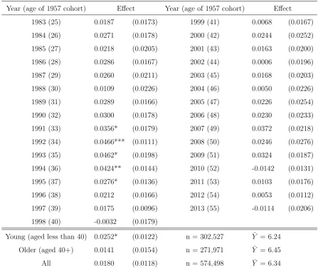
variation in the return to education over the life cycle. Table 2 reports estimates by year

and thus tracks out returns over the life cycle. For example, the first estimate is for 1983

when the 1957 cohort is aged 25 (and the 1952-1962 cohorts used in estimation are aged

between 20 and 30). The final estimate is for 2013 at which point the 1957 cohort is

aged 55 and the cohorts used in estimation are aged between 50 and 60. The estimates

2% at younger ages. Evidence for positive returns is weak for men over age 40 and the

coefficient is even negative in a few of the later years.16

In Table 2 we also show results where we pool across ages. First, we take average

log(weekly pay) across all years for each cohort and then use it as the dependent variable.

The resultant coefficient of 0.018 is not statistically significant but implies a return to an

extra year of education of about 6%. This is similar to what other researchers have found

for this law change using other data sets (Grenet (2013), Dickson (2012)).17 We also split the sample in two into a younger group (when the 1957 cohort is aged 25 to 39) and an

older group (when the 1957 cohort is aged 40 to 55) and report separate estimates for

these two groups. Consistent with the life cycle patterns, the point estimate is somewhat

larger for the younger group. Figures 3 - 5 provide a visual impression of these estimates

by plotting out average log(weekly pay) by cohort. There is a clear pattern of earnings

falling with cohort for younger men. This presumably arises because they are on the

upward sloping part of their life cycle earnings profile.

It is important to note that while our sample gets older as we move to later survey

years, we cannot be sure that differences in estimates by age are true effects of ageing.

This is because the return to education could change across time even if the average age

of sample members was time invariant. One possible reason is secular changes in the

return to education that might arise because of technological change. Another is cyclical

effects that could arise if education influences how earnings respond to the business cycle.

We examine this directly later in the paper.

16_{While many studies have shown life cycle relationships between education and earnings, we are}

only aware of two studies that show causal estimates by detailed age. Using a very different estimation

method, Buscha and Dickson (2015) show a broadly similar pattern of increasing then decreasing returns

using the NESPD. Our estimates are, however, in contrast to results from Norway which show that the

returns are typically lower at the beginning of the life cycle and higher at the end (Bhuller et al. 2017).

However, the authors note in their paper that these types of estimates are likely to vary across national

and institutional settings.

17_{Grenet (2013) uses the Quarterly Labour Force Survey from 1993 to 2004 and finds a return of 6-7%}

Table 2: Effect of the Law on Log Weekly Pay

Year (age of 1957 cohort) Effect Year (age of 1957 cohort) Effect

1983 (25) 0.0187 (0.0173) 1999 (41) 0.0068 (0.0167)

1984 (26) 0.0271 (0.0178) 2000 (42) 0.0244 (0.0252)

1985 (27) 0.0218 (0.0205) 2001 (43) 0.0163 (0.0200)

1986 (28) 0.0286 (0.0167) 2002 (44) 0.0006 (0.0196)

1987 (29) 0.0260 (0.0211) 2003 (45) 0.0168 (0.0203)

1988 (30) 0.0109 (0.0226) 2004 (46) 0.0050 (0.0226)

1989 (31) 0.0289 (0.0166) 2005 (47) 0.0226 (0.0254)

1990 (32) 0.0300 (0.0178) 2006 (48) 0.0230 (0.0233)

1991 (33) 0.0356* (0.0179) 2007 (49) 0.0372 (0.0218)

1992 (34) 0.0466*** (0.0111) 2008 (50) 0.0246 (0.0276)

1993 (35) 0.0462* (0.0198) 2009 (51) 0.0324 (0.0187)

1994 (36) 0.0424** (0.0144) 2010 (52) -0.0142 (0.0131)

1995 (37) 0.0276* (0.0136) 2011 (53) 0.0103 (0.0176)

1996 (38) 0.0212 (0.0166) 2012 (54) 0.0053 (0.0112)

1997 (39) 0.0175 (0.0096) 2013 (55) -0.0114 (0.0206)

1998 (40) -0.0032 (0.0179)

Young (aged less than 40) 0.0252* (0.0122) n = 302,527 Y¯ = 6.24

Older (aged 40+) 0.0141 (0.0154) n = 271,971 Y¯ = 6.45

All 0.0180 (0.0118) n = 574,498 Y¯ = 6.34

All regressions done at the cohort level. Standard errors in parentheses. Significance level: *** at

.01, ** at .05 and * at .10. ¯Y refers to the sample mean of the dependent variable.

5.2

Earnings Variability

Table 3 shows the effects of the law on the standard deviation of earnings over the life

cycle. Because, we can only estimate this for the middle year in each rolling 5-year period,

we have estimates by year from 1985 to 2011. What is immediately clear from the table

is that most of the effect of the law on earnings variability happens at young ages with

law exposure leading to less variability. There are large effects of the law around age

27-32 in the range of about 0.01. The average standard deviation for the 1957 cohort

Given an effect of the law change on education of about 0.30 to 0.35, this implies that

an extra year of education decreases earnings volatility by around 0.03 or by about 20%

of the mean which is quite a large effect. However, the size of the effect gets smaller

as men age and many of the point estimates even become positive (albeit statistically

insignificant) as men approach their 50s. One interpretation of this pattern is that more

education helps people to find better and more stable job matches in their early career but

the effect becomes unimportant at older ages when most individuals have found suitable

job matches. Of course, as mentioned earlier, an alternative possibility is that these are

time rather than age effects and that education particularly sheltered workers during the

1985-1990 period. While we can’t rule out this possibility, the general pattern seems

more consistent with an age rather than a cyclical effect.

As in Table 2, we also report estimates where we increase precision by pooling across

age groups. We find a statistically significant effect of -0.0065 for men aged less than

40 but no evidence of any effect for older men. We can assess whether these estimates

are statistically different using a Hausman test: Under the null hypothesis that there

is no difference between young and old, using the full sample provides a consistent and

efficient estimator for the young (or old) while, under the alternative hypothesis, it gives

inconsistent estimates for each individual group. Using this test, we find that the young

and old estimates are statistically different at the 10% level. Over the entire life cycle,

the average effect is -0.0042 but this estimate is not statistically significant.

Figures 6 - 8 provide a visual impression of these estimates. While the discontinuity

is obvious for younger men, there is no obvious jump in the older sample. Note that there

is a clear pattern of earnings variability rising with cohort for younger men, presumably

because earnings variability falls with age as workers become more settled into the labour

Table 3: Effect of the Law on the Standard Deviation of Log Earnings

Year (age of 1957 cohort) Effect Year (age of 1957 cohort) Effect

1985 (27) -0.0110*** (0.0029) 1999 (41) -0.0057 (0.0050)

1986 (28) -0.0118 (0.0066) 2000 (42) -0.0069*** (0.0019)

1987 (29) -0.0081 (0.0056) 2001 (43) -0.0044 (0.0057)

1988 (30) -0.0111*** (0.0024) 2002 (44) -0.0045 (0.0050)

1989 (31) -0.0101*** (0.0025) 2003 (45) -0.0001 (0.0057)

1990 (32) -0.0067 (0.0055) 2004 (46) 0.0033 (0.0059)

1991 (33) -0.0050 (0.0034) 2005 (47) 0.0009 (0.0070)

1992 (34) -0.0014 (0.0057) 2006 (48) -0.0037 (0.0053 )

1993 (35) -0.0042 (0.0062) 2007 (49) -0.0088 (0.0060)

1994 (36) -0.0049 (0.0040) 2008 (50) -0.0015 (0.0039)

1995 (37) -0.0047 (0.0047) 2009 (51) -0.0008 (0.0066)

1996 (38) -0.0060 (0.0034) 2010 (52) 0.0033 (0.0073)

1997 (39) -0.0045 (0.0034) 2011 (53) 0.0064 (0.0048)

1998 (40) -0.0062 (0.0044)

Young (aged less than 40) -0.0065** (0.0026) n = 197,741 Y¯ = 0.142

Older (aged 40+) -0.0022 (0.0027) n = 175,943 Y¯ = 0.122

All -0.0042 (0.0025) n = 373,684 Y¯ = 0.132

Standard deviations measured in the 5-year period centred around the listed year with at least 4

observations per window. Local linear regression estimates using cohorts born between 1952 and

1962 with the 1957 cohort omitted. All regressions done at the cohort level. Standard errors in

parentheses. Significance level: *** at .01, ** at .05 and * at .10. ¯Y refers to the sample mean of

the dependent variable.

In the estimates so far, we require at least 4 wage observations per person in each

5-year window. In Table 4, we examine whether the estimates are sensitive to using

different requirements. First, looking at the sample sizes, we see that as we move from

the least restrictive (only requiring 2 observations) to the most restrictive (requiring all

5), we lose over half the person-year observations. However, the estimates are quite robust

– the effect of the law on the younger group varies between -0.0063 and -0.0071 and is

always statistically significant. Likewise, there is never any evidence of an effect on the

Table 4: Effect of the Law on the Standard Deviation of Earnings

Effect Sample Size Sample Mean

SD calculated using at least 2 obs

Young -0.0064** (0.0026) 255,679 0.1467

Old -0.0018 (0.0028) 235,281 0.1266

All -0.0041 (0.0025) 490,960 0.1371

SD calculated using at least 3 obs

Young -0.0063** (0.0026) 238,787 0.1446

Old -0.0021 (0.0024) 218,468 0.1245

All -0.0040 (0.0024) 457,255 0.1350

SD calculated using at least 4 obs

Young -0.0065** (0.0026) 197,741 0.1416

Old -0.0022 (0.0027) 175,943 0.1221

All -0.0042 (0.0025) 373,684 0.1325

SD calculated using at least 5 obs

Young -0.0071* (0.0031) 126,388 0.1343

Old 0.0010 (0.0024) 111,500 0.1144

All -0.0031 (0.0026) 237,888 0.1250

All regressions done at the cohort level. Standard deviations measured in the 5-year period centred

around the listed year. Local linear regression estimates using cohorts born between 1952 and 1962

with the 1957 cohort omitted. Standard errors in parentheses. Significance level: *** at .01, ** at

Figure 3: Log Weekly Pay, Young Figure 4: Log Weekly Pay, Old

Figure 5: Log Weekly Pay, All Figure 6: Standard Deviation, Young

5.3

Earnings Cyclicality

As mentioned earlier, we calculate an earnings cyclicality coefficient for each cohort. To

estimate the effect of the law on earnings cyclicality, we do a cohort-level regression

where we regress the cyclicality coefficient for each cohort on the law using the local

linear specification. The estimates are reported in Table 5.

Because we need a large time dimension to reliably estimate the earnings cyclicality

coefficients, we cannot study how the effect of the law on earnings cyclicality varies at

each individual age. We report estimates for the full set of years (1983-2013) and also

split the sample by age group (younger versus older) as before. In practice, we estimate

earnings cyclicality over the 1983-1997 period when studying the younger group and the

1998-2013 period for the older group. However, the standard errors are very high for the

older group so this estimate is not very informative. In Table 5 we see that the effect

of the law on earnings cyclicality is about 0.0039 overall and, similarly, about 0.0044 for

the younger group. Both these estimates are large and very statistically significant. The

positive coefficient implies that law exposure reduces the negative relationship between

changes in earnings and changes in the unemployment rate.

Table 5: Effect of the Law on Earnings Cyclicality

Sample Effect Sample Size Sample Mean

Young (aged less than 40) 0.0044*** (0.0008) 223,974 -0.0037

Older (40+) 0.0005 (0.0054) 202,412 0.0123

All 0.0039*** (0.0008) 441,890 -0.0012

Local linear regression estimates using cohorts born between 1952 and 1962 with the 1957 cohort

omitted. All regressions done at the cohort level. Standard errors in parentheses. Significance level:

*** at .01, ** at .05 and * at .10.

To get a sense of the magnitudes, it is helpful to look at Figures 9 - 11. The pictures

show the estimated earnings cyclicality coefficient by cohort. For young men, this is

always negative, reflecting the fact that earnings are mildly procyclical with estimates

unemployment rate reduces earnings by between 0 and 0.7% and indicate considerably

larger cyclical sensitivity for later cohorts. For the full sample, the divergence across

cohort is smaller at between about 0 to -0.003. The greater procyclicality experienced by

those born in the early-to-mid 1960s may result from the fact that they were relatively

young during the turbulent decade of the 1980s and younger workers are more sensitive to

cyclical shocks.18 _{However, it is difficult to establish a precise reason for the cohort trends}

using our data. There is a clear jump for the 1958 cohort with the levels of cyclicality

being lower (in absolute terms) after the law change than before.

5.3.1 Regional Shocks

Table 6: Effect of the Law on Regional Earnings Cyclicality

Sample Effect Sample Size Sample Mean

Young (aged less than 40) 0.0038*** (0.0007) 223,974 -0.0039

Older (40+) 0.0010 (0.0052) 202,412 0.0107

All 0.0034** (0.0010) 441,890 -0.0013

The cyclical indicator is the contemporaneous regional unemployment rate for April. All regressions

done at the cohort level. Standard errors in parentheses. Significance level: *** at .01, ** at .05 and

* at .10.

Table 6 shows the regional cyclicality estimates. The results are similar to the estimates

using the national unemployment rate both in terms of the coefficient estimates and

standard errors. This is not surprising since Figure 1 highlights that unemployment rates

tend to move in parallel across regions. However, it is reassuring that, once we look

within region and so control for any regional effects, the negative effect of the law change

on earnings cyclicality remains.

18_{Much research has found that younger people are more sensitive to the business cycle, for example,}

Figure 9: Cyclicality, Young Figure 10: Cyclicality, Old

Figure 11: Cyclicality, All Figure 12: Regional Cyclicality, Young

5.4

Pay Cuts

Table 7 shows the effect of the law on the probability of a real pay cut in each 5-year

period centred on the reported year. We define the pay cut variable to be equal to 1 if the

real weekly pay at the end of the 5-year period is less than what it was at the beginning

of the period. So, for example, for the year 1987 in Table 7, the estimate shows the effect

of law exposure on the probability that the real weekly pay in 1989 is lower than that

in 1985. There is no clear pattern in the results with law exposure leading to a lower

probability of receiving a cut in some years, for example, in 1989, 1992 and 2004 but at

other times leading to an increased likelihood of a pay cut. The effect of education on

lowering the probability of receiving a pay cut in 1992 is consistent with the fact that

the 1990’s recession had large adverse effects on those with the least education. It is

not clear why the effects in 2004 are so large but it is something that we think deserves

further investigation. The increased probability of the higher educated receiving a pay cut

between 2007 and 2011 (as shown by the 2009 estimate) is consistent with evidence that

the ‘Great Recession’ had a bigger impact on those with more education, in particular

bankers and those working in the financial industry.19

Overall the effect of the law is to reduce the probability of a pay cut by 1.09 percentage

points. The average probability of a pay cut for the 1957 cohort over the sample period

is 0.342. Therefore, a coefficient of -0.0109 implies about a 3.2% reduction. This implies

that an extra year of education reduces the probability of receiving a pay cut by about

9 percent. However, it is important to keep in mind that there is a lot of heterogeneity

across years with positive coefficients in some years and negative ones in others so the

average effects over the entire period should be treated with caution. Figures 15 – 17

show the estimates graphically.

19_{This is not surprising given that in 2009 financial institutions reacted to the Lehman Brothers’}

Table 7: Effect of the Law on the Probability of a Real Weekly Pay Cut (over 5-Year

Period)

Year (age of 1957 cohort) Effect Year (age of 1957 cohort) Effect

1985 (27) -0.0150 (0.0109) 1999 (41) -0.0210 (0.0121)

1986 (28) -0.0260 (0.0133) 2000 (42) -0.0236 (0.0218)

1987 (29) 0.0001 (0.0169) 2001 (43) 0.0010 (0.0195)

1988 (30) -0.0122 (0.0103) 2002 (44) 0.0087 (0.0150)

1989 (31) -0.0195* (0.0096) 2003 (45) -0.0176 (0.0288)

1990 (32) -0.0288 (0.0216) 2004 (46) -0.0616*** (0.0162)

1991 (33) 0.0001 (0.0158) 2005 (47) -0.0111 (0.0202)

1992 (34) -0.0299* (0.0143) 2006 (48) -0.0451 (0.0330)

1993 (35) -0.0049 (0.0152) 2007 (49) -0.0071 (0.0176)

1994 (36) 0.0171* (0.0076) 2008 (50) -0.0000 (0.0155)

1995 (37) 0.0381* (0.0181) 2009 (51) 0.0447* (0.0191)

1996 (38) 0.0259 (0.0221) 2010 (52) 0.0279 (0.0207)

1997 (39) -0.0118 (0.0100) 2011 (53) 0.0180 (0.0149)

1998 (40) -0.0074 (0.0164)

Young (aged less than 40) -0.0081* (0.0037) n = 157,710 Y¯ = 0.260

Older (aged 40+) -0.0093 (0.0065) n = 195,484 Y¯ = 0.407

All -0.0109* (0.0046) n = 353,194 Y¯ = 0.342

Local linear regression estimates using cohorts born between 1952 and 1962 with the 1957 cohort

omitted. All regressions done at the cohort level. Standard errors in parentheses. Significance level:

Figure 15: Probability of Pay Cut, Young

Figure 16: Probability of Pay Cut, Old

6

Robustness Checks

In this section, we perform some robustness checks for each of our outcome measures.

The estimates are reported in the Appendix.

6.1

Bandwidth and Model Specification

First, we look at the effects of changing the bandwidth and the model specification. To

compare with our baseline estimates that do local linear regression using a bandwidth of 5,

we examine the effect of bandwidths of 7 and 10 using a range of different specifications.

Since the fit can vary greatly between specifications, we use the Akaike Information

Criterion (AIC) to pick the model that fits best in each case. With the bandwidth of

5, the standard errors get very high when we use high order polynomials. Therefore,

for this bandwidth, we only report a global quadratic in addition to the local linear

specification. For bandwidths 7 and 10, we report local quadratic estimates that allow a

different quadratic function each side of the discontinuity and also global quadratic, cubic,

and quartic specifications. In each case, the estimate favoured by the AIC criterion is

reported in bold.

The estimates are in Tables A1 to A5. In general, we find that, once one chooses

the specification with the best fit for each bandwidth, the estimates are quite robust to

specification. The estimates for the standard deviation, for earnings cyclicality, and (to

a lesser extent) for pay cuts are all quite similar across bandwidths for the best-fitting

model. We conclude that our findings are quite robust to the choice of bandwidth or

specification.

Because persons born in 1957 may or may not have been subject to the new law, we

have used a “donut” approach that involved excluding the 1957 cohort from the analysis.

In Table A6 we take an alternative approach of setting the law variable equal to 1/3

for the 1957 cohort. This reflects the fact that men born in September and after were

affected and they constitute approximately 1/3 of the cohort. We find that the estimates

are quite similar using this specification. One exception is that the effect of the law on

taking a real pay cut is no longer statistically significant. The lack of robustness of this

for this variable across years.

As mentioned earlier in the paper, we have missing observations for each of the

depen-dent variables because of non-employment, self-employment, and non-response. Here, we

investigate whether the law can predict whether there is missing data on the dependent

variables. We use the same local linear specification as for our main estimates. As can

be seen in Table A7, we find that there is no evidence for any systematic relationship

between the law and whether the dependent variables are missing. This finding is

con-sistent with our earlier result that the estimates for the standard deviation are robust

to variation in the number of required observations for each person over the five-year

period. While this evidence cannot be definitive, it suggests that our estimates may not

be biased by selection issues.

6.2

Looking Beyond Weekly Earnings

Our measure of weekly earnings depends both on average hourly earnings and weekly

hours worked. Given that the log of weekly earnings equals the sum of the logs of each

of these two variables, we look at the effect of the law change on each of these in turn.

Note that weekly hours are reported by employers and reflect contracted hours including

overtime hours. As shown in Table A8, we find very little evidence that hours variation

is an important part of the story – exposure to the law has little effect on hours or our

measures of hours variability. Indeed, the findings for the log hourly wage are fairly

similar to those for weekly earnings, suggesting that the law mainly impacts weekly

earnings through its effects on average hourly earnings.

From 1996, the NES has reported a measure of annual earnings with the current

employer that encapsulates the 12-month period ending at the survey date in April. We

use this variable for our “older” sample for the 1998-2013 period. We would expect the

estimates to differ from those for weekly earnings if there is significant variation in hours

worked over the year. In Table A9, we show estimates with this earnings measure along

with estimates for weekly earnings for the exact same sample of men. The estimates are

generally very similar and reinforce our earlier finding that the law appears to have little

6.3

Standard Errors Clustered at the Individual Level

We have conducted all our analysis at the cohort level. An alternative approach to

inference is not to group by cohort but to instead treat deviation from the local linear

or polynomial fit as specification error and report robust standard errors (Chamberlain,

1994). In situations where we pool years and so have repeated observations on individuals,

we implement this method by clustering by individual. As a check on our earlier estimates,

we report these standard errors in Tables A10 to A12. Given that earnings cyclicality

is measured at the cohort level, it is not possible to generate standard errors at the

individual level for this outcome. We find that the level of statistical significance is

generally similar with this approach compared to our earlier approach. All our findings

are robust to using this alternative method of inference.

7

Conclusion

We look at the effects of education on earnings volatility via the effects on earnings

vari-ability, earnings cyclicality, and frequency of real pay cuts of employed men. Across all

three mechanisms, the results point towards benefits from education through sheltering

men from the adverse effects of earnings shocks. We find that more education leads to

lower earnings variability at younger ages but with no discernible benefits for persons

aged over 40. We also find that more educated men are less affected by wage

cyclical-ity. Our findings for real pay cuts are quite heterogeneous with the effects varying in

magnitude and sign across different years. On average, however, more educated workers

appear less likely to experience real pay cuts. The estimates are robust across many

spec-ifications. Overall, our paper identifies another, and largely unexplored, avenue through

References

Altonji, Joseph G. 1993. The demand for and return to education when education

out-comes are uncertain. Journal of Labor Economics 11, no. 1:48–83.

Athreya, Kartik and Eberly, Janice C. 2015. The college premium, college

noncom-pletion, and human capital investment. Working Paper No. 13-02R, Federal Reserve

Bank of Richmond.

Ammermueller, Andreas., Anja. Kuckulenz and Thomas. Zwick. 2009. Aggregate

un-employment decreases individual returns to education. Economics of Education Review

28:217–226.

Banks, James, Richard Blundell and Agar Brugiavini. 2001. Risk pooling, precautionary

saving and consumption growth. Review of Economic Studies 68(4): 757-79.

Barcellos, Silvia, Leandro Carvalho and Patrick Turley. 2017. Genetic heterogeneity

on the health returns to education. Working paper.

Bhuller, Manudeep., Magne Mogstad and Kjell G. Slavanes. 2017. Life Cycle

Earn-ings, Education Premiums, and Internal Rates of Return. Journal of Labor Economics

35(4): 993-1030.

Bils, Mark J. 1985. Real wages over the business cycle: Evidence from panel data.

Journal of Political Economy 93, 666-689.

Blundell, Richard, Luigi Pistaferri, and Ian Preston. 2008. Consumption inequality

and partial insurance. American Economic Review 98(5): 1887-1921.

Blundell, Richard, Claire Crawford and Wenchao Jin. 2014. What can wages and

576, 377–407.

Blundell, Richard, Michael Graber and Magne Mogstad. 2015. Labor income dynamics

and the insurance from taxes, transfers, and the family. Journal of Public Economics

127:58–73.

Buscha, Franz and Matt Dickson. 2015. The wage returns to education over the life

cycle: Heterogeneity and the role of experience. Working Paper.

Chamberlain, G. 1994. Quantile regression, censoring, and the structure of wages. In:

Sims, C.A. (Ed.), Advances in Econometrics, Sixth World Congress, vol. 1. Cambridge

University Press, Cambridge.

Chen, Stacey. 2008. Estimating the variance of wages in the presence of selection and

unobserved heterogeneity. Review of Economics and Statistics 90:2, 275-289.

Cunha, Flavio, James Heckman and Salvador Navarro. 2005. Separating uncertainty

from heterogeneity in life cycle earnings. Oxford Economic Papers 57(2), 191-261.

Clark, Damon, and Heather Royer. 2013. The effect of education on adult mortality

and health: evidence from Britain”. American Economic Review 103(6): 2087-2120.

Delaney, Judith M. 2017. ”To go to college or not? The role of ability, family

back-ground, and risk”. Working Paper.

Devereux, Paul J. and Robert A. Hart. 2010. Forced to be rich? Returns to

com-pulsory schooling in Britain. The Economic Journal 120.549: 1345–1364.

Dickens, William T. 1990. Error components in grouped data: Is it ever worth

Dickson, M. 2013. The causal effect of education on wages revisited. Oxford Bulletin

of Economics and Statistics 75: 477–498.

Dolton, Peter and Matteo Sandi. 2017. Returning to returns: revisiting the British

education evidence. Labour Economics 48:87-104.

Donald, Stephen G., and Kevin Lang. 2007. Inference with difference-in-differences

and other panel data. The Review of Economics and Statistics 89.2: 221–233.

Elsby, Michael W., Bart Hobijn and Aysegul Sahin. 2010. The labor market in the

Great Recession. Published: Brookings Papers on Economic Activity, Economic Studies

Program, The Brookings Institution, vol. 41(1 (Spring), pages 1-69.

French, Eric. 2005. The effects of health, wealth, and wages on labour supply and

retirement behaviour. The Review of Economic Studies 72.2: 395–427.

Grenet, Julien. 2013. Is extending compulsory schooling alone enough to raise

earn-ings? Evidence from French and British compulsory schooling laws. The Scandinavian

Journal of Economics 115.1: 176–210.

Hahn, Jinyong., Petra Todd, and Wilbert. Van der Klaauw. 2001. Identification and

es-timation of treatment effects with a regression-discontinuity design. Econometrica 69(1):

201–209.

Harmon, Colm., and Ian Walker. 1995. Estimates of the Economic Return to Schooling

for the United Kingdom. American Economic Review 85: 1278-1286.

Heathcote, Jonathan, Kjetil Storesletten, and Giovanni L. Violante. 2014. Consumption

Review 104(7): 2075-2126.

Hines, James. R., Hilary Hoynes and Alan. B Krueger. 2001. Another look at whether

a rising tide lifts all boats. Working Paper no. 8412, National Bureau of Economic

Re-search, Cambridge, MA.

Hoynes. Hilary, Douglas L. Miller, and Jessamyn Schaller. 2012. Who suffers during

recessions?. Journal of Economic Perspectives 26(3): 27-48

Imbens, Guido W., and Thomas Lemieux. 2008. Regression discontinuity designs: A

guide to practice. Journal of Econometrics 142.2: 615–635.

Ionescu, Felicia and Nicole Simpson. 2016. Default risk and private student loans:

Impli-cations for higher education policies. Journal of Economic Dynamics and Control 64(C):

119-147.

Johnson, Matthew T. 2013. Borrowing constraints, college enrollment and delayed entry.

Journal of Labor Economics 31.4: 669–725.

Keane, Michael P., and Kenneth I. Wolpin. 1997. The career decisions of young men.

Journal of Political Economy 105.3.

Keane, Michael, and Answar Prasad. 1993. Skill levels and the cyclical variability of

employment, hours, and wages. International Monetary Fund Staff Papers 40, 711-743.

Liu, Kai, Magne Mogstad and Kjell Salvanes. 2015. Education, earnings dynamics,

and life cycle inequality. Working Paper.

Low, Hamish, Costas Meghir, and Luigi Pistaferri. 2010. Wage risk and employment

Machin, Stephen., Kjell. G. Salvanes, and Panu. Pelkonen. 2012. Education and

mobil-ity. Journal of the European Economic Association 10: 417–450.

Meghir, Costas and Luigi Pistaferri. 2004. ”Income variance dynamics and

heterogene-ity”. Econometrica 72:1–32.

Mincer, Jacob. 1991. Education and unemployment. NBER Working Paper No 3838.

National Bureau of Economic Research, Cambridge, MA.

Nickell, Stephen., Tracy Jones, and Glenda Quintini. 2002. A picture of job

insecu-rity facing British men. The Economic Journal 112: 1–27.

Oreopoulos, Philip. 2006. Estimating average and local average treatment effects of

education when compulsory schooling laws really matter. American Economic Review

96(1): 152-175.

Oreopoulos, Philip, and Kjell G. Salvanes. 2011. Priceless: The nonpecuniary

bene-fits of schooling. Journal of Economic Perspectives 25(1): 159-84.

Solon, Gary., Robert Barsky, and Jonathan A. Parker. 1994. Measuring the cyclicality

of real wages: How important is composition bias. The Quarterly Journal of Economics