Large eddy simulation of dispersion: comparison between elevated source and ground level source

between Elevated and Ground-Level Sources

Zhengtong Xie, Paul Hayden, Peter R. Voke and Alan G. Robins

Fluids Research Centre, School of Engineering, University of Surrey, Guildford GU2 7XH, U.K.

1. Abstract

Large-eddy simulation (LES) is used to calculate the concentration fluctuations of pas-sive plumes from an elevated source (ES) and a ground-level source (GLS) in a turbu-lent boundary layer over a rough wall. The mean concentration,relative fluctuations and spectra are found to be in good agreement with the wind-tunnel measurements for both ES and GLS. In particular,the calculated relative fluctuation level for GLS is quite satisfactory,suggesting that the LES is reliable and the calculated instantaneous data can be used for further post-processing. Animations are shown of the meandering of the plumes,which is one of the main features to the numerical simulations. Extreme value theory (EVT),in the form of the Generalised Pareto distribution (GPD),is ap-plied to model the upper tail of the probability density function of the concentration time series collected at many typical locations for GLS and ES from both LES and experiments. The relative maxima (defined as maximum concentration normalized by the local mean concentration) and return levels estimated from the numerical data are in good agreement with those from the experimental data. The relative maxima can be larger than 50. The success of the comparisons suggests that we can achieve significant insight into the physics of dispersion in turbulent flows by combining LES and EVT.

Key words: large-eddy simulation,atmospheric dispersion,plume meandering, rough wall,extreme value theory,generalized Pareto distribution,relative maxima.

2. Introduction

caused by the large turbulent eddies may make a critical contribution to the variance of concentration fluctuations [2].

In the light of these factors,research is necessary to develop basic understanding and to improve our predictive capability. Existing approaches for addressing these issues are limited. Over the past couple of decades large-eddy simulation (LES) has received increasing attention because of its ability to describe turbulence in more detail than closure models and its economy compared with direct numerical simulation. LES can contribute more to prediction of atmospheric flow and dispersion from sources as the meandering of the concentration plume and high intermittency of its fluctuations make the relative intensity of fluctuations even higher than 4.0 [2]. LES may be the most promising technical approach to simulating atmospheric flow and dispersion from small sources,because of the very large Reynolds number. Sykes et al. [11] applied LES to numerically generate statistics of the fluctuating concentration field downstream of a localized source of a passive scalar. Meeder and Nieuwstadt [5] also studied the dispersion of a reactive plume from an elevated small source in the neutral atmospheric boundary layer by means of LES.

High concentrations of pollutants in the atmosphere,although usually of very low frequency,can be dangerous to human health or can exceed flammability or explosion limits. Modelling their occurrence is a challenge. LES can provide instantaneous three dimensional flow and concentration data in the study of dispersion from a small source release. Unfortunately,we can normally only simulate ABL flows over a couple of hours (or wind tunnel flows over less than a minute) by LES,owing to current computer capabilities and the resulting high expense of extended simulations. Such a time duration cannot provide sufficient information to fix the upper tail of the probability density function (PDF),any more than normal experiments. Lack of detailed information of the upper tail of the PDF can make the standard estimation of extreme events severely biased.

Extreme value theory (EVT) is the branch of statistics concerned with modelling the tails of probability distributions and hence performing probability extrapolations. Classically,EVT [3] referred to the Three-Types Theorem for Maxima,with types I, II and III widely known as the Gumbel,Fr´echet and Weibull types respectively. The work was extended by von Mises [6] and Jenkinson [4],who independently derived the generalized extreme value distribution (GEV) of these three seemingly disparate families. A typical application of this model is to fit the distribution to a series of maximum data (for instance,annual maximum rainfall). However,the technique of characterizing a GEV distribution just by using maximum data during some fixed period is obviously of low efficiency. Several techniques,such as point process characterization,threshold methods,the Generalized Pareto Distribution (GPD) [8], ther-largest order statistics method and so on,which manage to take more data into account,have been proposed to obtain higher data-using efficiency.

3. LES for turbulent flow over a rough surface

We consider incompressible air flow over a rough surface at very high Reynolds number. In the horizontal directions the flow is periodic. At the top of the domain,stress free conditions are imposed. At the bottom boundary a wall model relates the surface stress to the tangential velocity components at the first inner grid point. A new wall model is proposed which exhibits more satisfactory performance than previous models for the LES of the turbulent boundary layer over a rough surface [15],which is written as follows,

τxz u2∗ =

1 Ua

< u >+β

(u−< u >)2n/2 un

∗ (u−< u >)

, n≥0, (1)

where Ua is the mean streamwise velocity at the first grid location from the wall, β is evaluated theoretically. Settingn= 0 recovers Thomas and Williams’s wall model [12]. The model withn= 2 appears to be close to optimal.

To quantify the subgrid viscosity,we use the mixed-scale model (MSM) of Sagaut [9]. The MSM expresses the subgrid viscosity in terms of the local strain-rate scalar S=2SijSij,the subgrid kinetic energyqand a filter width ∆,as follows:

νs(α) =cMSαq1−2α_∆1+α_.

The standard MSM of Sagaut [9] has α = 1/2 and the corresponding constant cM is equal to 0.064. The filter width is evaluated in a standard manner as ∆ = (∆x1∆x2∆x3)1/3. The subgrid kinetic energy qis estimated using a test filter as commonly employed in dynamic SGS procedures.

The momentum equations are discretized in space using a second-order central differencing finite-volume method. We use a staggered grid which is uniform in both horizontal directions and slightly stretched in the vertical direction. All quantities (including the passive scalar) are advanced in time through time splitting with two steps,giving a second-order explicit scheme.

The numerical results are judged by comparison with the wind tunnel measurements. We choose the boundary layer depth D and friction velocity u∗

as reference length and reference velocity. The computational domain size is 4D×1.375D×D. The roughness element height zh is 0.0125D and the roughness length z0 is 0.00114D. We discretise the computational domain on a fine mesh of

256×128×128,which is the default mesh; a medium mesh of 128×64×64 is also used for comparison. Some results are shown in figure 1,where the spectra are obtained at the heightz= 0.44D,which is the height of the elevated source.

4. LES for dispersion of small source release

The filtered governing equation of the scalar is written as follows, ∂c

∂t + ∂ujc

∂xj = ∂ ∂xj

(Ks+Km) ∂c ∂xj

(2)

0 5 10 15 20 25 1E-3

0.01 0.1

Z/

D

U/u*

0 2 4 6

0.0 0.2 0.4 0.6 0.8

Z/

D

TKE/u*

2

-5/3

1.0E-07 1.0E-05 1.0E-03 1.0E-01

1.0E+00 1.0E+01 1.0E+02 1.0E+03

E(f)/(Du

*

)

-5/3

1.0E-07 1.0E-05 1.0E-03 1.0E-01

1.0E+00 1.0E+01 1.0E+02 1.0E+03 f*D/u*

E(f)/(D/u

*

)

Figure 1. Left: Streamwise mean velocity. Lines, LES: solid, with new

wall model; dashed, with Schumann’s wall model; symbols, measurements. Center: Turbulent kinetic energy. Lines, LES: dashed, resolved; dotted, sub-grid; solid, total; symbols, measurements. Right: Spectra. Lines, LES; solid, fine mesh; dashed, medium mesh; symbols, measurements; top, of streamwise velocity; bottom, of vertical velocity.

dynamically. In the present study,we adopt the above concept using a constant Schmidt number with a value of 1.2,

Ks=νs/Sc,

where νs is the subgrid viscosity [15] and Sc is the Schmidt number. Numerical experiments have been performed to check the sensitivity to Schmidt number,from which we found values around 1.2 yields very small variations of the results. Km is small in our simulation,since the Reynolds number is large,but is nevertheless included.

The formulae of the SMART scheme are given as follows,based on the literature published by Waterson and Deconinck [14]:

cw = cW + 0.5∗B(r)∗(cW −cW W)

r = cP−cW cW−cW W

B(r) = max [0,min(2∗r,0.75∗r+ 0.25,4)].

(3)

To make the expression clear,in the above equation it is assumed that the instantaneous velocity is from west to east; thus cell W is on the upwind side of cellP,cellW W is on the upwind side of cellW,and wdenotes the west cell face of cellP. The LES code does not make that assumption and is more general.

0.01 0.1 1 10

0.01 0.1 1 10 100

Cpeak

/C

peak

(x

=0.

575D)

X/D

(a) Maximum mean concentration in the cross-plume plane.

0 2 4 6 8

0 1 2 3

crm

s

/C

peak

X/D

(b) Relative concentration fluctuations.

Figure 2. (a): – – LES ES;◦measurements ES; —– LES GLS;•measurements

GLS. (b): our measurements;Thomson’s stochastic model; – – LES ES; –·– extrapolated from LES ES; —– LES GLS; ◦measurements GLS;•Fackrell and Robins GLS.

LES predict larger relative intensities than Thomson’s model [13],which was proposed to suit homogeneous turbulence.

Turning to the comparison between measurements and LES,the difference may be accounted for in several ways,such as the slight difference of resolution and source size. For the GLS,the results are in good agreement with the current measurements and the experimental data of Fackrell and Robins [2]. Since the mean maximum concentration decreases approximately with a power law,figure 2 (a),the contribution of the background noise to crms in the experiments is not likely to be small; this is likely to be the main factor resulting in an overestimation of the relative concentration fluctuation at the point farthest downstream. However,we believe that the effect of the background noise can be reduced with improvement of the quality of the equipment.

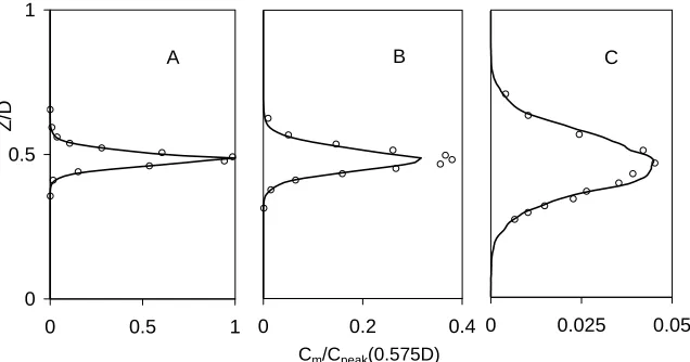
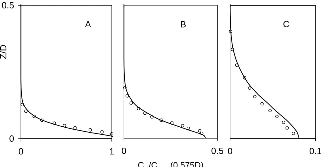
Vertical profiles of mean concentration andcrms/Cpeakare plotted in figure 3 for ES,and figure 4 for GLS. The comparison between LES results and measurements are quite reasonable. For the GLS,the maximum concentration at all downstream stations is always at ground level,though in figure 3(b) there are some random components in both LES results and measurements at the far downstream positions, owing to the limited sampling time. Referring to figure 4(b),for the GLS in the wind-tunnel experiment,the velocity of the flow from the source itself was bigger than the background mean velocity. Since the GLS background mean velocity is much smaller than at the ES height,it is very difficult to match the GLS background mean velocity. The effect of the jet is to make the turbulent mixing stronger for the GLS and it presumably makes the off-ground peak occur earlier in measurements than in the LES. On the other hand,although the numerical scheme is of low numerical diffusion and second-order accuracy,the mesh resolution very close to the source is not fine enough to fully resolve the plume,which may induce numerical errors. However,it must be pointed out that the measurements of Fackrell and Robins [2] also show a peak off the surface. At stations further downstream,the location of maximumcrms in the LES is in reasonable agreement with measurement.

A double-peak behaviour can be found in the lateral profiles of crms/Cpeak far downstream from the source (approximatelyx >0.95D) for the GLS. This is due to the fact that the size of the plume far downstream from the source is larger than that of the turbulence,making the location of the plume nearly fixed at ground level and making the meandering less. Hence,at the edge of the plume the concentration is highly intermittent. For the elevated source (ES),the scale of the plume is initially smaller than that of the turbulence,and so meandering plays a very important role.

Figure 5 shows that the time series of instantaneous concentration for ES and GLS are quite different from each other. The meandering of the plume plays a very important role for ES and consequently the intermittency is quite dramatic. In contrast the meandering is not as important for GLS since the vertical scale of the plume always exceeds that of the turbulence,and the vertical dispersion progresses as in the far field.

0 0.5 1

0 0.5 1

Z/D

A

0 0.2 0.4

Cm/Cpeak(0.575D)

B

0 0.025 0.05

C

(a) Vertical profiles of mean concentration.

0 0.5 1

0 1.8

Z/D

A

0 2.2

crms/Cpeak

B

0 2.3

C

(b) Vertical profiles ofc_rms/C_peak.

Figure 3. ES. A, x=0.575D; B, x=0.95D; C, x=2.7D. —– LES;◦measurements.

0 0.5

0 1

Z/D

A

0 0.5

Cm/Cpeak(0.575D)

B

0 0.1

C

(a) Vertical profiles of mean concentration, plume centre.

0 0.5

0 1

Z/D

A

0 0.8

crms/Cpeak

B

0 0.7

C

(b) Vertical profiles ofc_rms/C_peak.

Figure 4. GLS. A, x=0.575D; B, x=0.95D; C, x=2.7D. —– LES;◦measurements.

0 2 4 0

5 10

0 2 4

0 1 2

(A)

C/

Cm

t/(D/u_*)

(B)

C/

Cm

t/(D/u )

Figure 5. Instantaneous concentration time series at x/D=2.7 and at the height

of the source: (A) ES (B) GLS.

more evident in 6(b),while meandering in the lateral direction is weak. Disconnection of concentration clouds is never seen in 6(b).

(a) ES (b) GLS

Figure 6. Animations of 2-D contours of instantaneous concentration at the

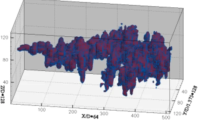
Figure 7(a) and 7(b) show animations of 3D contours of instantaneous concentration for ES and GLS respectively. The contour values for ES and for GLS are 10−4 and 5×10−5 respectively. The maximum mean concentrations for ES and for GLS at the farthest downstream station x/D= 8 are 1.8×10−4 and 1.1×10−4 respectively. The normalized durationTdU∞/Lx for ES is 1,while it is 1.5 for GLS.

Td is the animation duration. The dataset processed here is collected from an LES with mesh 512×128×128. Since there are hundreds to thousands of time steps to be stored,the dataset size can be hundreds of gigabytes. In order to save hard disk space,a technique was developed and applied in which only the concentration exceeding a threshold and the coordinates of the corresponding cell are sampled and recorded on hard disk for later post-processing,since only the concentration exceeding the threshold is of interest.

In the animation in figure 7(a),the plume twists and meanders dramatically in both vertical and lateral directions,particularly in the near-source area of the domain. The frequency of meandering and twisting is higher close to the source than far downstream. The frequency of meandering heavily influences the return period of the extreme concentration,discussed in detail in section 5. In the near-source region even small-scale turbulent eddies can convect the whole of a small plume efficiently, and the time scale of the small-scale turbulent eddy is normally small. Far downstream from the source,the size of the plume is larger and only the dominant large turbulent eddies can efficiently convect the whole plume and make the meandering evident. The time scale of the large scale turbulent eddies is normally large. Note that the amplitude of meandering of the plume in the vertical direction is in the same scale as that in the lateral direction. With the interaction of the meandering in lateral and vertical directions and the strong convection in streamwise direction,the dispersion of the plume near the source is modest in figure 7(a),which is also evident from the plot of plume width,figure 3. We also note in figure 7(b) the meandering is weak in the lateral direction,while in the vertical direction there is no meandering because of the presence of the wall. In the near-source area for GLS,the dispersion of the plume is stronger than that for ES.

5. EVT prediction

The Generalized Pareto Distribution is applied to model extreme events exceeding a high thresholduin the time series:

P rob(Γ≤u+φ|Γ> u) =Gξσ(φ) = 1−(1 + ξ σφ)

−1/ξ_{, (4)}

where Γ is physical quantity, φ, ξ and σ are argument,shape and scale parameters respectively,andσ >0,φ >0,1 +ξφ/σ >0. ξandσneed to be fitted by likelihood method [1]. It is known that ξ is independent of u,while σ depends linearly on u. Takingξ <0 for GPD to have a finite upper limit [7].

In environmental studies the quantity of most interest is the return level,which is defined (loosely) as the value which we expect will be exceeded on average once in a given period,i.e return period. A more precise definition of return level can be given [1]. Let τ denote the return period,ν is the crossing rate of the threshold u, r is the return level (noter > u). From equation 4,the average crossing rate of levelr isν1 +ξ(r−u)/σ)−1/ξ _{,which is set equivalent to 1/τ to obtain}

Where the return levelris independent of the thresholdu. Providedξ <0,the local maximum Γ₀ is deduced from the above equation:

Γ₀=u−σ/ξ. (6)

There is a trade-off in threshold choice: thresholds which are too low incur bias due to invalidity of the asymptotic argument; thresholds which are too high have few exceedances processed and so sampling variability is high. An useful diagnostic tool is to apply one characteristic of the GPD distribution [7],

E(Γ−u|Γ> u) = ξ(u−Γ0)

1−ξ , (7)

where E is the mean excess function,provided ξ < 0. This tool is realized by a mean excess plot in which the mean difference between the exceedances and the threshold against threshold is plotted. Hence,if the asymptotic approximation is correct,the mean excess plot should be a straight line with slopξ/(1−ξ) and intercept

−ξΓ₀/(1−ξ). Quantile quantile plots are also used to find a suitable threshold,and to check the goodness of fitting.

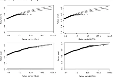
A simple numerical experiment was conducted to verify the utility of EVT. The dispersion of the ES release was calculated by LES on a coarse mesh up to several million time steps,while the instantaneous concentration was recorded. Time series with different durations (from 10 thousand to 3 million steps) were processed separately using EVT. The results are plotted in figure 8,where the EVT-predicted solid lines are quite comparable with one another,and the 95% confidence intervals tend to decrease with increasing duration. In particular,comparing the left-top figure with the right-bottom figure,the predicted return level (the solid line) at 500 normalized return period is nearly 0.7 in the former,while an observation (the last circle) at approximately 500 normalized return period is found close to 0.7 in the latter (forget the lines for the moment). This illustrates that the return period of the occurrence of an extreme event has been successfully predicted by EVT processing a short-duration time series.

In order to check the robustness of the predictions,the GPD parameters generated from fits to various durations of data,up to the maximum gathered,are compared. These series with different durations are processed using the same threshold and cluster time interval,and the shape parameterξand scale parameterσand the local maximum Γ₀ are studied as functions of the duration of data used for the fit. One typical example is shown in figure 9. Note the parameters tend to constants for the longer series durations,demonstrating the process is robust.

Recall that the shape parameterξis negative in the current case,which restricts the GPD to a finite upper limit. Lower ξ (larger absolute value) makes the return level approach the upper limit closely in a shorter return period (see equation 5). The parameter ξ tends to decrease with downstream distance for the GLS,which can be interpreted as evidence of meandering and intermittency quickly becoming much weaker further downstream (see figures 2 (b),6 and 7). However,the trend of parameter ξ further downstream for the ES is not as obvious for the GLS,perhaps owing to the short downstream distance. Much longer downstream distances may be needed to obtain certain trends of ξ for ES than that for GLS. Although the meandering and intermittency decrease gradually downstream for ES,seems this has no obvious impact on the tendency of the shape parameter.

Figure 10 shows the relative maxima and return levels at several downstream locations for GLS and ES,where the relative maxima and relative return levels are respectively defined as EVT-predicted maximum concentration (upper limit Γ₀,see equation 6) and return levels normalized by local mean concentration. Despite the large confidence intervals for LES,the relative maxima and return levels for LES are all in good agreement with those for the measurements,except the comparison at X/D= 2.7 for ES. Note that the relative maxima are over 40 for ES at X/D= 2.7. Compared with figure 10A for GLS,the magnitude and the trend against downstream distance of the relative maximum in figure 10C for ES are quite different. This suggests that the turbulence has a large effect on the extreme concentrations,since the local turbulence in the near wall region is quite different from that at the height of the ES. We note that figure 10C is very similar in shape to the plot of relative intensity of fluctuations for ES,where the peak is located aroundX/D= 2.0 as well. Sykeset al.

[11] pointed out that the relative intensity of the fluctuations for an ES decays towards zero downstream. In figure 10C,there is an evident decay downstream. However,the trend far downstream for both relative intensity and relative maximum for GLS still remains an issue. From the current LES data and measurements for the GLS (see figure 2),the relative intensity has a very slight drop atx/D = 1.0. Downstream of x/d= 2.0 it clearly approaches a constant. The relative maximum still has a slight drop beyondx/D= 4.0,which makes the downstream trend not so obvious.

We note that far downstream the local maximum Γ₀ is approached in a shorter duration than close to the source. Note that the far downstream time series are ’denser’(fewer zeros or very low concentration values and more peaks) due to the weak meandering and intermittency. From such a time series,less ξ(larger absolute value) is obtained; hence,the return level approaches the upper limit more closely in a return period (see equation 5).

single cell,which may induce some numerical errors very close to the source. This may be manifest as an effectively larger source in the near-source area. We note that close to the source,the effects of source size are remarkable,while far from the source this effects tend to disappear. Fackrell and Robins [2] investigated the source size effects by means of wind tunnel measurement; they found the maximum relative intensity ranging between 1.3 and 5. They also found the influence of the source size decreases further downstream.

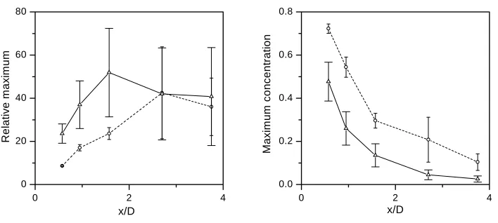
In current paper,more attention is paid to the the source size effect on the extreme concentration. Since the source size influences the meandering dramatically, the meandering effect on the concentration maxima also is studied here. Figure 11 shows the source size effect on the concentration maxima (upper limit). In figure 11 (right),the maximum concentration for the bigger source is higher than that for the normal size source over the whole distance,owing to the larger volume of passive scalar released at the inflow boundary in the former case. In figure 11 (left),the source size effect is quite evident close to the source. The relative maxima for the normal size source are much larger than those for the bigger source. Since the meandering of the plume is more important for a smaller size source,we ascribe the dramatic difference to the meandering. Further downstream from the source,the size effect becomes less important because the meandering becomes weaker and plays a less important role.

6. Conclusion and discussion

Concentration dispersion from elevated and ground-level sources over a rough wall has been investigated by comparing numerical data from large-eddy simulation with measurements. Our success in simulating fluctuation levels for ES and GLS indicates that our wall model,SGS model and numerical scheme are quite satisfactory.

The significant difference between the two cases previously found in experiment is realized successfully in large-eddy simulation. Furthermore,this difference is intensively investigated comparing the relative concentration fluctuations and the animations of contours of instantaneous concentration. In particular,the meandering, which contributes greatly to the relative concentration fluctuations and the relative maxima,can be considered a key to differentiating the scalar field for the ES from that for the GLS.

References

[1] Davison A C and Smith R L 1990 Models for exceedances over high thresholds (with discussion)

J. R. Statist. Soc. B52393-442

[2] Fackrell J E and Robins A G 1982 Concentration fluctuations and fluxes in plumes from point sources in a turbulent boundary layerJ. Fluid Mech.1171-26

[3] Fisher R A and Tippett L H C 1928 Limiting forms of the frequency distribution of the largest or smallest member of a sampleProc. Cambridge Phil. Soc.24180-190

[4] Jenkinson A F 1955 The frequency distribution of the annual maximum (or minimun) values of meteorological elementsQ. J. Roy. Meteorol.87158-171

[5] Meeder J P and Nieuwstadt F T M 2000 Large Eddy simulation of the turbulent dispersion of a reactive plume from a point source into a neutral atmospheric boundary layerAtmospheric Environment343563-3573

[6] Mises R von 1954 La distribution de la plus grande de n valeurs In selected papers II pp271-294 Providence RI: mer. Math. Soc.

[7] Munro R J, Chatwin P C and Mole N 2001 The high concentration tails of the probability density function of a dispersing scalar in the atmosphereBound.-Layer Meteorol.98315-339 [8] Picands J 1975 Statistical inference using extreme order statisticsAnn. Statist.3119-131 [9] Sagaut P 1995‘Simulations num´eriques d’´ecoulements d´ecoll´es avec des mod`eles de sous-maille’

PhD Thesis, University of Paris VI, France

[10] Smith R L 1989 Extreme value analysis of environmental time series: an application to trend detection in ground-level ozoneStatist. Sci.4367-393

[11] Sykes R L and Henn D S 1992 LES of concentration fluctuations in a dispersing plumeAtmos. Env.26A3127-3144

[12] Thomas,T.G and Williams J.J.R. 1999 Generation of a wind environment for large-eddy simulation of bluff body flows.J. Wind Eng. & Indust. Aerodyn.82, 189-208.

[13] Thomson D J 1990 A stochastic model for the motion of particle pairs in isotropic high-Reynolds-number turbulence and its application to the problem of concentration variance J. Fluid Mech.,210113-153

[14] Waterson N P and Deconinck H 1995 A unified approach to the design and application of bounded higher-order convection schemes, in ‘Numerical Methods in Laminar and Turbulent Flows’Proceedings of the Ninth International Conference( ed. Taylor C. and Durbetaki P.)

9Part 1 203-214

(a) ES

(b) GLS

Figure 8. Return level extrapolation. LES, very coarse mesh; from left to right, then top to bottom, 104,105,106,3×106 time steps respectively. Circles, LES data. Lines, EVT predicted with 95% confidence intervals.

0.0 0.4 0.8

-1.0 -0.8 -0.6 -0.4 -0.2

ξ

T_p/T_tlt

0.0 0.4 0.8

4.0x10-5 6.0x10-5 8.0x10-5

σ

T_p/T_tlt

0.0 0.4 0.8

1.0x10-4 2.0x10-4 3.0x10-4 4.0x10-4

Γ0

T_p/T_tlt

Figure 9. Parameters fitted from short-term and long-term series at the station

0 4 8 0 2 4 6 8 10 12 A re la tiv e m a x im u m o r re tu rn le v e l x/D

0 4 8

0 2 4 6 8 B x/D

0 2 4

0 20 40 60 80 re la tiv e m a x im u m o r re tu rn le v e l _C x/D

0 2 4

0 20 40 60 D x/D

Figure 10. Relative maxima and return levels. Bars: 95% confidence

0 2 4 0

20 40 60 80

R

e

la

tive

m

a

xim

u

m

x/D

0 2 4

0.0 0.2 0.4 0.6 0.8

Max

im

u

m

concent

ra

ti

on

x/D

Figure 11. Source size effect on maximum concentration. Vertical bars: 95%