Design method for ultimate efficiency in linear cavity continuous wave lasers using distributed feedback

(1)

ePrints Soton

copyright owners. A copy can be downloaded for personal non-commercial

research or study, without prior permission or charge. This thesis cannot be

reproduced or quoted extensively from without first obtaining permission in writing

from the copyright holder/s. The content must not be changed in any way or sold

commercially in any format or medium without the formal permission of the

copyright holders.

When referring to this work, full bibliographic details including the author, title,

awarding institution and date of the thesis must be given e.g.

AUTHOR (year of submission) "Full thesis title", University of Southampton, name

of the University School or Department, PhD Thesis, pagination

(2)

Faculty of Engineering, Science & Mathematics

Optoelectronics Research Centre

Design Method for Ultimate Efficiency in

Linear-cavity Continuous-wave Lasers

Using Distributed-Feedback

by

Kuthan Yelen

Thesis Submitted for the Degree of Doctor of Philosophy

(3)

OPTOELECTRONICS RESEARCH CENTRE Doctor of Philosophy

DESIGN METHOD FOR ULTIMATE EFFICIENCY IN LINEAR-CAVITY CONTINOUS-WAVE LASERS

USING DISTRIBUTED-FEEDBACK by Kuthan Yelen

A novel analytical method for the design of linear-cavity continuous-wave laser cavities

that guarantees the ultimate efficiency is developed, theoretically studied and

experimentally verified. Opposed to the earlier methods, which optimise the parameters

of a priori defined cavity, the developed method derives the cavity analytically based on

the active medium properties for the chosen pumping scheme. The method combines the

general grating design equations, valid for both passive and active media, and the

optimum signal power calculations. The idea that lies at the heart of the design method is

to sustain the optimum signal power at every single point in the entire cavity by

employing distributed-feedback for the maximum local, as a result, for the maximum

overall conversion efficiency.

Theoretical study starts with the critical investigation of the previous optimisation

approaches. After addressing the limitations of these approaches, it is shown how to

improve the efficiency further than the parametric optimisation using intuitive arguments

based on the effective cavity length and optimum reflectivities in DFB lasers. The critical

importance of the signal distribution is highlighted, and following this observation the

grating design method for arbitrary signal distributions is developed. The concept of

optimum signal power is introduced and the spatial unfolding of the optimum values is

illustrated. Boundary conditions, grating production limitations and effects of modelling

parameters are addressed. Modal stability of the new designs is investigated.

A novel approach to the simulation of Er/Yb co-doped fibre lasers is presented with

experimental justification. Accurate laser characteristics are predicted for different

designs, including the ultimate efficiency designs. Theoretical studies are verified with

experimental data in Er/Yb co-doped fibre and discussions are extended to Yb doped

(4)

List of Abbreviations

ASE

Amplified

Spontaneous

Emission

CUP

Co-operative

Up-Conversion

DBR

Distributed Bragg Reflector

DFB

Distributed Feedback

ESA

Excited-state

Absorption

FP

Fabry-Perot

JAC

Jacketed

Air

Cladding

LHS

Left-hand

side

NA

Numerical Aperture

PM

Power

Meter

RHS

Right-hand

side

TLS

Tunable Laser Source

(7)

List of Symbols

Symbol Value

or

[Unit] Description

Subscripts

s

At signal wavelength

p

At pump wavelength

n

Normal

ytterbium

ions

q

Lifetime

quenched

ytterbium

Ions

Subscripts

a

Absorption

e

Emission

C

ESA

[

m

2

]

Excited

state

absorption

cross-section

C

UP

[

m

3

s

-1

] Co-operative

up-conversion

coefficient

D

[ m ]

Penetration depth (Chapter 5)

D(z)

[ W ]

Difference between forward and backward

propagating powers at position z

E [

_{W m}2

]

Total electric field (Normalised)

Er

i

[]

Single erbium ion at energy level i

G

[ W ]

Generated signal power over a volume

∆

G(z)

[ W / m ]

Generated signal per unit length at position z

k

tr

[

m

3

s

-1

]

Energy transfer coefficient between Er

and Yb ions

L

[ m ]

Total device length

L

eff

[

m

]

Effective

cavity

length

n

0

[]

Effective refractive index of the medium

∆

n

[]

Refractive

index

modulation

amplitude

n

1

[]

Refractive

index

of

the

core

n

2

[]

Refractive

index

of

the

cladding

N

T

[

m

-3

]

Total

ion

concentration

(8)

P(z)

[ W ]

Pump power at position z in a laser cavity

∆

P(z)

[ W / m ]

Absorbed pump power per unit length

P

p

[ W ]

Pump power in an amplifying medium

P

s

[ W ]

Signal power in an amplifying medium

r

[]

Reflection

coefficient

R

[]

Reflectivity

R

+

[

_{W m}2

]

Forward Propagating Electric Field Envelope

(Normalised)

R

-

[

_{W m}2

]

Backward Propagating Electric Field Envelope

(Normalised)

S(z)

[ W ]

Sum of forward and backward propagating

powers at position z

Yb

i

[]

Single

ytterbium

ion

at

energy

level

i

z

[ m ]

Position

z

π

[ m ]

Position of the phase-shift

α

[

m

-1

]

Field gain (positive) or loss (negative)

coefficient

β

[

m

-1

]

Propagation

constant

Γs,p

[]

Overlap coefficient for signal or pump

field

Γ

[

m

-1

]

Phase difference between the fields and the

grating

ε

[

m

-1

]

Field

background

loss

Λ

[

m

]

Period

of

the

grating

η

[]

Pump-to-signal

conversion

efficiency

κ

(z)

[

m

-1

]

Coupling coefficient of the grating at position z

λ

[

m

]

Wavelength

ν

[

s

-1

]

Frequency

σ

[

m

2

]

Cross-section

τi

[ s ]

Life-time at energy level i

(9)

To my aunt Ayfer Özbeyli, for her contributions to my life… Teyzem Ayfer Özbeyli’ye, hayatımdaki - destekten öte - katkılarına minnetle…

ACKNOWLEDGEMENTS

With ample amount of coffee and the ability to survive some not-so-easy periods

any stubborn person can complete a PhD. However, enjoying the entire PhD

experience requires more than being determined; you have to be lucky. A sensible

initial point

, years-long non-fading guidance, and a harmony with your

supervisor in terms of both academic approach and personality are what it takes

to make your postgraduate life enjoyable. With the wisdom of hindsight, I can see

that I was one of the luckiest persons around. For all these, I thank my supervisor

Professor Michalis Zervas heartily.

Playing with equations, pushing the simulations to the limits, and the feeling of

being the only person, at that particular moment, who knows what it is all about,

is fantastic. But making things actually work in reality is even more satisfying.

Louise Hickey is the person who made it possible for me to link all the theory to

the physical world. I would like to thank Louise and the personnel of

Southampton Photonics, SPI Inc. for the icing on the cake. Writing up the thesis is

another story. Avoiding

writers’ cramp

by

hitting the gym,

I finally finished the

thesis and dear Eleanor Tarbox kindly allocated her valuable time to correct my

countless mistakes.

(10)

“

The purpose of computing is

insight, not numbers.

”

(11)

(12)

1.1. Motivation

Improving the efficiency of lasers is of great importance throughout the entire

optoelectronics field. As well as being a fundamental research interest, better laser

efficiency is a very strong commercial driver too. Today, linear-cavity continuous-wave

(CW) lasers are one of the most widely used types of lasers that come in categories such

as semiconductor, solid-state, fibre and planar glass. Therefore maximizing the efficiency

of this particular type of lasers is very desirable and will have a broad impact in the

optoelectronics field.

The performance of a laser is set by various characteristics of the device such as the

active medium spectroscopy, temperature control mechanism and pumping scheme. One

of the most critical features of a laser that has profound effect on the efficiency is the

design of the resonator cavity. The structure of the cavity defines the circulating power,

the amount of output coupling and the extracted output power. For a given pump power

and active medium under the same operating conditions different laser cavities yield

different efficiencies; therefore the cavity design lies at the heart of laser performance.

The simplest form of a linear cavity laser is the classic Fabry-Perot (FP) type laser, which

comprises two mirrors and an active medium in between, whereas the most complex

linear cavity is the distributed feedback (DFB) laser, which incorporates a grating into

the active medium. A distributed Bragg reflector (DBR) or a FP laser can be treated as a

sub-set of DFB lasers: In the case of a DBR laser the coupling coefficient of the grating in

the active medium is reduced to zero, but it is extended into the passive section. In the

case of a FP laser the coupling is localised at the ends of the active medium by placing

infinitesimal gratings; that is mirrors.

Optimisation of the cavity design for FP lasers dates back to the well- known Rigrod

analysis [1, 2]. This analytical optimisation, however, is based on very limiting

assumptions and simplifications: First of all, the unsaturated gain is assumed to be

(13)

for example, be valid for electrically side-pumped semiconductor lasers however this

assumption excludes many other pumping schemes. Then the active medium is assumed

to be a homogenously saturated 2-level system. Optimisation of a FP laser cavity

constructed in this medium assumes very small output coupling from the end mirrors

(very high reflectivity) and very small saturated gain. With these assumptions the

circulating signal inside the cavity is almost constant and with an additional assumption

of constant loss the optimum output coupling and the optimum circulating signal are

found analytically (For example see [3]).

Any deviation from any of these assumptions, which is almost always the case for any real

system, causes the analytical Rigrod optimisation to break down. In the case of a

multi-level active medium with varying signal and pump powers or signal dependent loss a

parametric optimisation is required; that is one of the cavity parameters is varied at a

time while the others are kept constant and the laser is simulated for the output powers

using numerical techniques.

A FP laser cavity is defined by only three parameters: the two mirror reflectivites and the

cavity length. Therefore, a parametric optimisation, although computationally intense,

can consider all the possible combinations. But the FP cavity is not the only possible laser

configuration, hence the efficiency maximised for a FP design is not guaranteed to be the

maximum possible for the given medium and pump power. Other laser structures such as

distributed Bragg reflector (DBR) or distributed feedback (DFB) configurations may

provide better efficiencies under comparable conditions. However optimisation of these

complex structures parametrically is even more challenging since there are literally an

infinite number of combinations of parameters when apodisation profile, chirp profile,

total length and phase shift positions and amounts are considered; therefore the

parametric optimisation cannot guarantee the maximum efficiency possible for the given

pump and active medium. A maximum may be a local peak in efficiency over an infinite

number of different parameter combinations.

To sum up, there is a lack of a general comprehensive design method for widely used

linear cavity CW lasers which would assure the fundamental efficiency limit analytically.

In this work we present a novel analytical method for the design of laser cavities. In our

approach we do not optimise a certain laser cavity but we derive the cavity for a given

(14)

1.2. Approach

Being the most complex and general cavity, DFB lasers will provide the starting point for

our study. We will critically investigate the classic DFB laser optimisation approach in

order to improve our understanding of the effects of cavity design on the laser

performance. Observing the importance of the signal distribution in the cavity and

experimentally verifying its effect, we will introduce the concept of the optimum signal

and continue with the method for achieving the optimum signal distribution in the entire

cavity. Then imposing the boundary conditions and production limitations and employing

the novel grating design method we will show how to find the coupling coefficient profile

which provides this signal distribution.

The method does not discriminate between the Fabry-Perot, DBR or DFB structures,

however, in general, the maximum efficiency laser cavity requires a distributed feedback;

consequently the method is applicable to any active medium in which a grating can be

incorporated. Therefore we expect this design method to find immediate application over

a wide device range from semiconductor, planar glass, solid-state bulk to fibre lasers

since in these media the grating writing technologies have already matured.

As a demonstration we applied the method experimentally in Er/Yb co-doped fibre lasers.

We chose this particular medium because of the attractive feature of fibre DFB lasers

that we will cover in Chapter 2.

1.3. Modelling and Simulations

To facilitate the theoretical and the experimental investigations we use numerical models

extensively, both for the derivation of the laser designs and their simulation. Therefore,

the model and the simulation tools we developed are an essential part of our study.

Although several entirely theoretical works on modelling of erbium-ytterbium co-doped

media have been reported [4-10] with only very few experimental verifications for

amplifiers [11, 12] there is no work on benchmarking the simulation results with

experimental results for Er/Yb co-doped lasers, neither in FP, DBR or DFB configuration.

The value of any simulation result should be judged according to its proximity to the

behaviour of the real device or system. If the performance of a model is not checked

against the experimental data then the simulation results will make sense only in terms of

tendencies instead of actual numbers.

Here, in addition to the novel design method, we present a model for Er/Yb co-doped

(15)

up conversion in erbium ions as well as the life-time quenching of ytterbium ions. We

describe simple techniques for the measurement of the model parameters. In this new

modelling approach we treat the pump, the active medium and the feedback mechanism

as a complete system, and we characterise and model each one of them. For the first

time, we present simulations that predict the actual characteristics of the Er/Yb co-doped

DFB fibre lasers within the range of experimental measurement errors.

1.4. Overview of the Thesis

Following this introduction chapter, an overview of fibre DFB lasers is presented in

Chapter 2, followed by the brief description of numerical and computational methods

used throughout the rest of the study in Chapter 3. The modelling of the active medium

and DFB lasers are discussed in Chapter 4. The transitions and the rate equations are

discussed in detail and the measurement of the required parameters as well as the

characterisation of the pump source and the grating are presented. Results of the

simulations are compared against the experimental data.

Chapter 5 is devoted to the detailed investigation of the classic DFB laser optimisation

method. It is shown that, the method is equivalent to the Rigrod analysis for the

reflectivities, however in addition to the feedback the signal distribution inside the cavity

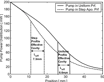
is identified as a critical variable affecting the efficiency. The concept of effective cavity is

introduced and the step-apodised profile is presented to increase the effective cavity

length for better efficiency. The theoretical results are verified with the experimental

data.

Identification of the signal distribution as a critical factor for the laser efficiency leads to

the general theoretical analysis for a design method in order to achieve any desired signal

distribution inside passive and active cavities in Chapter 6. Here we discuss the optimum

signal distribution for the maximum possible efficiency and we illustrate the new design

method in a numerical study in a simple ytterbium doped fibre.

Chapter 7 covers the theoretical and experimental application of the design method in

erbium-ytterbium co-doped fibre. Initially, designs for alternative pumping schemes are

derived and compared, longitudinal-mode stability is discussed, and the effects of the

uncertainties in the model parameters on the design are investigated, then the method is

experimentally verified. High power applications along with alternative pump and signal

(16)

Concluding remarks on the design method are presented in Chapter 9. References are

given at the end of each chapter.

1.5. References

[1] W. W. Rigrod, "Saturation Effects in High-Gain Lasers," Journal of Applied

Physics, vol. 36, no. 8, pp. 2487-2490, 1965.

[2] C. T. Meneely, "Laser Mirror Transmissivity Optimization in High Power Optical

Cavities," Applied Optics, vol. 6, no. 8, pp. 1434-1436, 1967.

[3] A. E. Siegman, "Section 12.3," in LASERS. Sausalita, CA: University Science

Books, 1986.

[4] C. Strohhofer and A. Polman, "Relationship between gain and Yb3+ concentration

in Er3+ - Yb3+ doped waveguide amplifiers," Journal of Applied Physics, vol. 90,

no. 9, pp. 4314-4320, 2001.

[5] E. Yahel and A. Hardy, "Modeling and Optimization of Short Er3+-Yb3+ Codoped

Fiber Lasers," IEEE Journal of Quantum Electronics, vol. 39, no. 11, pp.

1444-1451, 2003.

[6] E. Yahel and A. Hardy, "Modeling High-Power Er3+ - Yb3+ Codoped Fiber

Lasers," Journal of Lightwave Technology, vol. 21, no. 9, pp. 2044-2052, 2003.

[7] M. Karasek, "Optimum Design of Er3+-Yb3+ Codoped Fibers for Large-Signal

High-Pump-Power Applications," IEEE Journal of Quantum Electronics, vol.

33, no. 10, pp. 1699-1705, 1997.

[8] G. C. Valley, "Modeling Cladding-Pumped Er/Yb Fiber Amplifiers," Optical Fiber

Technology, vol. 7, no. 1, pp 21-44, 2001.

[9] F. Di Pasquale, "Modeling of Highly-Efficient Grating-Feedback and Fabry-Perot

Er3+ Yb3+ Co-Doped Fiber Lasers," IEEE Journal of Quantum Electronics, vol.

32, no. 2, pp. 326-332, 1996.

[10] J. Nilsson, P. Scheer, and B. Jaskorzynska, "Modeling and Optimization of Short

Yb3+ Sensitized Er3+ Doped Fiber Amplifiers," IEEE Photonics Technology

Letters, vol. 6, no. 3, pp. 383-385, 1994.

[11] G. Sorbello, S. Taccheo, and P. Laporta, "Numerical modelling and experimental

investigation of double-cladding erbium-ytterbium-doped fibre amplifiers," Optical and Quantum Electronics, vol. 33, no. 6, pp 599-619, 2001.

[12] M. Achtenhagen, R. J. Beeson, F. Pan, B. Nyman, and A. Hardy, "Gain and Noise

in ytterbium-Sensitized erbium-Doped Fiber Amplifiers: Measurements and

Simulations," Journal of Lightwave Technology, vol. 19, no. 10, pp. 1521-1526,

(17)

(18)

2.1. Historical Perspective

The discovery of lasing in periodic structures dates back to the early 70s. Kogelnik and

Shank, then at the Bell Laboratories, reported lasing action in a dyed gelatine whose

refractive index was periodically modulated [1]. Figure 2-1 illustrates the earliest DFB

laser structure. The laser consists of a uniform refractive index grating, with constant

amplitude and constant period, incorporated in an active medium. This classic design

operates at two fundamental longitudinal modes at different wavelengths, corresponding

to the edges of the grating band-gap, and gives symmetric output powers from both ends,

Pleft and Pright, which are equally divided between these two modes. Therefore, such a

cavity provides dual-wavelength bi-directional operation.

Figure 2-1 Refractive index profile for classic DFB laser design with two-wavelength bi-directional operation.

The theory of lasing action in periodic structures was developed in the classic paper,

again by Kogelnik and Shank, based on coupled-wave theory [2].

After this initial observation of lasing action in the periodic structures, the second

mile-stone leading to fibre DFB lasers came with the discovery of the formation of permanent

gratings in photosensitive germania-doped fibres by Hill et al [3] of the Canadian

Communications Research Centre in 1978. The grating was formed by the interference

pattern of argon-ion laser radiation propagating in opposite directions in the fibre. This

method required that in order to write a Bragg grating at a certain wavelength one would

need to launch a field at the same wavelength longitudinally into the fibre, therefore the

wavelength of the Bragg grating was limited with the available source wavelengths.

The major breakthrough came from Meltz, Morey and Glenn, working at the United

Technologies Research Centre, in 1989 [4]. In their holographic approach the grating was

(19)

produced by exposing the photosensitive fibre transversely to the interference pattern

produced by two intersecting UV beams. By doing so, the period of the grating became a

function of the angle between the beams, hence gratings with any periodicities could be

written. This holographic writing approach found application in erbium doped fibre. Ball

and Morey from United Technologies Research Centre and Zyskind et al from AT&T Bell

Laboratories reported Er doped DBR laser structures in 1992 [5, 6]. Further

improvements in grating writing techniques followed in 1993 by the introduction of phase

masks in order to produce the UV interference pattern demonstrated by Hill et al [7] and

Anderson et al of AT&T Bell Laboratories[8]. The phase-mask method reduced the

mechanical sensitivity of the writing setup and allowed the introduction of apodisation

and chirping profiles.

The next breakthrough, again in 1993, was the sensitisation of the erbium ions by

co-doping with ytterbium. Kringlebotn et al, from the Optoelectronics Research Centre of

Southampton University showed that the introduction of Yb ions dramatically increased

the pump absorption [9]. This discovery made short fibre lasers feasible and efficient.

However there was one problem: The highly absorbing Yb required the use of a

phosphosilicate host which reduces the photosensitivity, as opposed to the

germanosilicate host used for Er-only doped fibres. In 1994 the same research group

from Southampton University solved this problem by loading the aluminophosphosilicate

fibre with hydrogen to induce photosensitivity. They produced the first Er/Yb co-doped

DFB fibre laser by combining the holographic grating writing method and the hydrogen

loaded photosensitive active fibre technology [10]. Although the fibre suffered from

hydrogen related losses they were able to obtain laser action. Contrary to the

dual-wavelength output from the classic DFB cavity, in practice, a single-dual-wavelength operation

is desired. This can be achieved by introducing a π-shift in the spatial phase of the grating

as shown below. Such a cavity provides a single-wavelength, coinciding with the grating

Bragg wavelength, and bi-directional operation.

Figure 2-2 Symmetric, π-phase shifted DFB laser design for single-wavelength operation with bi-directional outputs.

Kringlebotn et al managed to introduce the necessary phase-shift by heating the grating

locally with a thin resistance wire. Although this approach provided the single-mode

operation desired, the induced phase shift was not a permanent feature of the grating.

(20)

In 1995 Cole, Loh et al from Southampton University improved the phase-mask method

further [11, 12]. In their approach the fibre was moved relative to the phase mask while

the writing beam was scanning. This method allowed the use of simple short phase

masks, as opposed to the earlier, stationary, custom designed phase mask, and the

required grating periodicity, phase-shift, apodisation and chirping profiles were produced

by precisely controlling the position of the successive exposures to the UV interference

pattern. This method greatly reduced the errors in the grating and allowed flexibility for

the production of complex grating structures. 1995 witnessed the announcement of Er

doped DFB fibre lasers with a permanent phase-shift simultaneously from two research

groups. The studies by Loh and Laming from Southampton University [13] and Sejka et al

from Technical University of Denmark [14] defined the point where DFB fibre production

technology reached maturity. Once the basics of the technology had been established the

efforts were focused around the optimisation of the fibre and the cavity designs in the

following years.

Dong et al from Southampton University showed that a better fibre for DFB lasers would

be one with a photosensitive cladding. Instead of loading the core with lossy hydrogen to

get improved photosensitivity, they produced a boron and germanium-doped

photosensitive cladding surrounding the active phosphosilicate core doped with Er and

Yb [15], thus boosting the laser efficiency greatly in 1997.

At the end of 90s, Lauridsen et al [16, 17] and Ibsen et al [18] showed that a better cavity

design would be composed of an optimum combination of grating strength and an

asymmetrically positioned phase-shift so that the uni-directional output power is the

maximum. By placing the phase-shift asymmetrically with respect to the grating centre,

as shown in Figure 2-3 larger output power is obtained from the closer end.

Figure 2-3 Refractive index profile for asymmetric π-phase shifted DFB laser design for single-wavelength uni-directional operation.

Today a typical state of art Er/Yb DFB laser is 5 cm long and produces around 20 mW

output power at 1550 nm when pumped with 100 mW at 980 nm and is limited to 50 mW

output power even when pump powers as large as 650 mW are used [19].

P

left

(21)

2.2. Applications

The fibre DFB lasers possess certain unique properties that make them more attractive

compared to the semiconductor lasers. First of all they are in-fibre lasers therefore they

are inherently fibre compatible and their output can be connected to a transmission fibre

using a standard splice. Similarly, the pump power can be delivered to the fibre DFB

laser using simple low-loss transmission fibres. In addition, very simple passive thermal

stabilisation is sufficient to ensure the stability of a fibre DFB laser. A number of different

active dopants, such as erbium, ytterbium, neodymium and thulium, can be used in order

to cover different windows of the optical spectrum and offer extended coverage.

These features, combined with the ability to define the emitted wavelength precisely, a

narrow linewidth and a low relative intensity noise (RIN), make DFB fibre lasers very

advantageous for telecommunication applications [20-22]. Typically an Er/Yb doped laser

has a linewidth less than 50 kHz, much smaller compared to 1MHz of a conventional

semiconductor laser. The RIN figure in such lasers is less than 100 dB/Hz above 50MHz,

and the signal-to-noise ratio is larger than 65 dB. In addition to these advantages, a

number of DFB fibre lasers can be configured in a parallel array to provide flexibility in

pumping conditions and provide pump redundancy [23].

Various methods have been demonstrated to ensure robust single polarisation operation

of fibre DFB lasers [24-26]. This robust single polarisation operation and stable

wavelength with narrow linewidth are very desirable for sensor systems. Alternatively,

DFB lasers can be made to operate in stable dual-polarisation so that simultaneous

measurements can be carried out [27-29]. In addition to the sensing and telecom

applications, we recently demonstrated the high power application of DFB fibre lasers

[30] following the advances in the pump source technologies.

2.3. References

[1] H. Kogelnik and C. V. Shank, "Stimulated Emission in a Periodic Structure,"

Applied Physics Letters, vol. 12, no. 18, pp. 152-154, 1971.

[2] H. Kogelnik and C. V. Shank, "Coupled-wave Theory of Distributed Feedback

Lasers," Journal of Applied Physics, vol. 43, no. 5, pp. 2327-2335, 1972.

[3] K. O. Hill, Y. Fujii, D. C. Johnson, and B. S. Kawasaki, "Photosensitivity in Optical

Fiber Waveguides: Application to Reflection Filter Fabrication," Applied Physics

Letters, vol. 32, no. 20, pp. 647-649, 1978.

[4] G. Meltz, W. W. Morey, and W. H. Glenn, "Formation of Bragg Gratings in Optical

Fibers by a Transverse Holographic Method," Optics Letters, vol. 14, no. 15, pp.

823-825, 1989.

[5] G. A. Ball and W. W. Morey, "Continuously Tunable Single-Mode erbium Fiber

(22)

[6] J. L. Zyskind, V. Mizrahi, D. J. DiGiovanni, and J. W. Sulhoff, "Short Single

Frequency erbium-Doped Fiber Laser," Electronics Letters, vol. 28, no. 15, pp.

1385-1387, 1992.

[7] K. O. Hill, B. Malo, F. Bilodeau, D. C. Johnson, and J. Albert, "Bragg Gratings

Fabricated in Monomode Photosensitive Optical Fiber by Uv Exposure through a

Phase Mask," Applied Physics Letters, vol. 62, no. 10, pp. 1035-1037, 1993.

[8] D. Z. Anderson, V. Mizrahi, T. Erdogan, and A. E. White, "Production of in-Fiber

Gratings Using a Diffractive Optical- Element," Electronics Letters, vol. 29, no. 6,

pp. 566-568, 1993.

[9] J. T. Kringlebotn, P. R. Morkel, L. Reekie, J. L. Archambault, and D. N. Payne,

"Efficient Diode-Pumped Single Frequency erbium:ytterbium Fiber Laser," IEEE

Photonics Technology Letters, vol. 5, no. 10, pp. 1162-1164, 1993.

[10] J. T. Kringlebotn, J. L. Archambault, L. Reekie, and D. N. Payne, "Er3+Yb3+

Codoped Fiber Distributed-Feedback Laser," Optics Letters, vol. 19, no. 24, pp.

2101-2103, 1994.

[11] M. J. Cole, H. Geiger, R. I. Laming, S. Y. Set, M. N. Zervas, W. H. Loh, and V.

Gusmeroli, "Broadband dispersion-compensating chirped fibre Bragg gratings in a 10Gbit/s NRZ 110km non-dispersion-shifted fibre link operating at 1.55 mu m," Electronics Letters, vol. 33, no. 1, pp. 70-71, 1997.

[12] W. H. Loh, M. J. Cole, M. N. Zervas, S. Barcelos, and R. I. Laming, "Complex

Grating Structures with Uniform Phase Masks Based on the Moving

Fiber-Scanning Beam Technique," Optics Letters, vol. 20, no. 20, pp. 2051-2053, 1995.

[13] W. H. Loh and R. I. Laming, "1.55 um phase-shifted distributed feedback fibre

laser," Electronics Letters, vol. 31, no. 17, pp. 1440-1442, 1995.

[14] M. Sejka, P. Varming, B. Hubner, and M. Kristensen, "Distributed feedback Er3+

doped fibre laser," Electronics Letters, vol. 31, no. 17, pp. 1445-1446, 1995.

[15] L. Dong, W. H. Loh, J. E. Caplen, J. D. Minelly, K. Hsu, and L. Reekie, "Efficient

single-frequency fiber lasers with novel photosensitive Er/Yb optical fibers," Optics Letters, vol. 22, no. 10, pp. 694-696, 1997.

[16] V. C. Lauridsen, J. H. Povlsen, and P. Varming, "Design of DFB fibre lasers,"

Electronics Letters, vol. 34, no. 21, pp. 2028-2030, 1998.

[17] V. C. Lauridsen, J. H. Povlsen, and P. Varming, "Optimising erbium-doped DFB

fibre laser length with respect to maximum output power," Electronics Letters,

vol. 35, no. 4, pp. 300-302, 1999.

[18] M. Ibsen, E. Ronnekleiv, G. J. Cowle, M. O. Berendt, O. Hadeler, M. N. Zervas, and

R. Laming, "Robust high power (>20mW) all-fibre DFB lasers with unidirectional and truly single polarisation outputs," presented at CLEO, Baltimore, USA, 1999,CWE4

[19] K. H. Yla-Jarkko and A. B. Grudinin, "Performance Limitations of High-Power

DFB Fiber Lasers," IEEE Photonics Technology Letters, vol. 15, no. 2, pp.

191-193, 2003.

[20] J. Hubner, P. Varming, and M. Kristensen, "Five wavelength DFB fibre laser

source for WDM systems," Electronics Letters, vol. 33, no. 2, pp. 139-140, 1997.

[21] M. Ibsen, S. U. Alam, M. N. Zervas, A. B. Grudinin, and D. N. Payne, "8-and

16-channel all-fiber DFB laser WDM transmitters with integrated pump redundancy," IEEE Photonics Technology Letters, vol. 11, no. 9, pp. 1114-1116, 1999.

[22] H. N. Poulsen, P. Varming, A. Buxens, A. T. Clausen, P. Munoz, P. Jeppesen, C. V.

Poulsen, J. E. Pedersen, and L. Eskildsen, "1607 nm DFB fibre laser for optical communcation in the L-band," presented at ECOC, Nice, France, 1999, MoB2.1

[23] L. B. Fu, S. R., M. Ibsen, J. K. Sahu, J. N. Jang, S. U. Alam, J. Nilsson, D. J.

Richardson, D. N. Payne, C. Codemard, S. Goncharov, I. Zalevsky, and A. B. Grudinin, "Fiber-DFB laser array pumped with a single 1-W CW Yb-Fibre Laser," IEEE Photonics Technology Letters, vol. 15, no. 5, pp. 655-657, 2003.

[24] Z. E. Haratjunian, W. H. Loh, R. I. Laming, and D. N. Payne, "Single Polarization

Twisted Distributed Feedback Fiber Laser," Electronics Letters, vol. 32, no. 4,

(23)

[25] H. Storoy, B. Sahlgren, and R. Stubbe, "Single polarisation fibre DFB laser," Electronics Letters, vol. 33, no. 1, pp. 56-58, 1997.

[26] J. L. Philipsen, M. O. Berendt, P. Varming, V. C. Lauridsen, J. H. Povlsen, J.

Hubner, M. Kristensen, and B. Palsdottir, "Polarisation control of DFB fibre laser

using UV-induced birefringent phase-shift," Electronics Letters, vol. 34, no. 7, pp.

678-679, 1998.

[27] J. T. Kringlebotn, W. H. Loh, and R. I. Laming, "Polarimetric Er3+-doped fiber

distributed-feedback laser sensor for differential pressure and force

measurements," Optics Letters, vol. 21, no. 22, pp. 1869-1871, 1996.

[28] O. Hadeler, E. Ronnekleiv, M. Ibsen, and R. I. Laming, "Polarimetric Fiber

Distibuted Feedback Laser Sensor for Simultaneous Strain and Temperature

Measurements," Applied Optics, vol. 38, no. 10, pp. 1953-1958, 1999.

[29] O. Hadeler, M. Ibsen, and M. N. Zervas, "Distributied-feedback fiber laser sensor

for simultaneous strain and temperature mesurements operating in the

radio-frequency domain," Applied Optics, vol. 40, no. 19, pp. 3169-3175, 2001.

[30] C. A. Codemard, L. Hickey, K. Yelen, D. B. S. Soh, R. Wixey, M. Coker, M. N.

(24)

(25)

3.1. Introduction

As in the case of any simulation, the accuracy and the computation time are the two

issues that have to be balanced in the calculation of the DFB laser characteristics. In this

Chapter we will discuss the algorithms that allowed us to simulate gratings, rare-earth

doped fibres and fibre lasers, typically with computation times less then 1 minute for

device lengths up to 10 cm, using a standard PC with Pentium® 4 1.2GHz processor and

128 Mb RAM. Matlab© Ver. 6.1. was used for the implementation of the algorithms

because of its very high performance for matrix-based calculations and the readily

available mathematical library.

The simulation of a device requires the solution of two groups of equations, namely; the

propagation equations for fields in the grating and the rate-equations of the active

medium. When the grating apodisation profile is suitably defined, solution of these two

sets of equations enables the simulation of fibre lasers with FP, DBR or DFB structures.

In addition to the power characteristics, we can also simulate the laser threshold

conditions and longitudinal signal and pump distributions.

Passive gratings can also be simulated by setting the loss to a constant value. In this case

the reflection, transmission and time-delay spectra can be calculated. Alternatively, the

grating can be ignored by setting the coupling coefficient to zero and free propagation in

the rare-earth doped medium can be simulated.

3.2. Simulation of Propagation in Grating Structures

The main requirement for the simulation algorithm for propagation is the ability to work

on any kind of grating, with arbitrary apodisation and chirp profiles, as well as with an

arbitrary number of discreet phase-shifts, so that it will be possible to compare very

different laser designs in our quest for maximum efficiency. For this purpose we

(26)

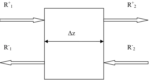
tool for the analysis of complex laser structures [1-5]. The essence of the method is to

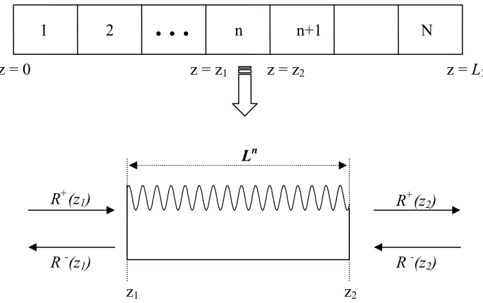
divide a complex structure into small segments so that each segment can be assumed to

[image:26.595.141.493.165.386.2]

be uniform, as illustrated in Figure 3-1.

Figure 3-1 Transfer matrix method. A complex grating with arbitrary

apodisation and chirping profile and discrete phase shifts is divided into N

small segments so that each segment is approximately uniform.

If

Ψ

+(x,y)and

Ψ

-(x,y) are the transverse modal distributions, where (+) and (-) signs

indicate the direction of propagation, then the total electric field E(x,y,z) at a position is

( , , ) ( ) ( , ) ( ) ( , )

E x y z =E z+ Ψ+ x y +E z− Ψ− x y . The transfer matrix, T, of a uniform segment relates the electric fields on one side of the segment to the fields on the other side in the

form:

1 11 12 2

21 22

1 2

( )

E z

T

E z

T

E z

+ +

− −













=

































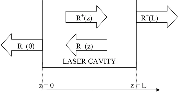
(3.1)

We use the electric field amplitude envelopes, R(z), to separate the slowly varying part

form the fast modulated term,

e

βz and re-write the total electric field as:

( , , ) ( ) ( , ) i z ( ) ( , ) i z

E x y z =R z+ Ψ+ x y e−β+ +R z− Ψ− x y eβ− (3.2)

where

β

+ and

β

– are the propagation constants of the forward and backward propagating

fields, respectively.

R

+

(z

1

)

R

-

(z

1

)

R

+

(z

2

)

R

-

(z

2

)

z

1

z

2

L

n

1 2

. . .

n n+1 N

(27)

Starting from the coupled-wave equations, as given by Equations (6.2) and (6.3), the

entries of the T-matrix for the uniform grating segment, n, in Figure 3-1 between z = z1

and z = z2 of length Ln are found as [2]:

( )

11

'

cosh

sinh(

)

i BLn

n n

i

n

T

γ

L

β

γ

L

e

β

γ



∆



=



+







(3.3)

( )

12

sinh(

)

n n B

i L

n n

T

κ

γ

L e β φ

γ

− +

−

= (3.4)

( )

21

sinh(

)

n n B

i L

n n

T

κ

γ

L e β φ

γ

+ −

= (3.5)

( )

22

'

cosh

sinh(

)

i BLn

n n i n

T

γ

L

β

γ

L e β

γ

−

 ∆ 

=_ − _

  (3.6)

where

∆β

’

,

γ

and

φ

n are defined as:

(

)

2 2 1 1 ' ' 2 n n j initial j j i L

β

β α

γ

κ

β

π

φ

−

= ∆ = ∆ + = − ∆   = + _ _ Λ  

∑

(3.7)

Here

φ

_initial is the initial phase of the grating at z = 0 and

Λ

is the period of the segment.

∆β

is the deviation from the propagation constant,

β

B

=

2πn0/

λ

B

,

at the Bragg wavelength

of the segment, given as

λ

B

= 2

n0

Λ

where n0 is the effective refractive index of the

medium. In the equations positive

α

is the gain experienced by the field.

φ

n is a

piece-wise approximation of the grating phase defined in Equation (6.4) while the sinusoidal

refractive index modulation given by Equations (6.6) results in the coupling coefficient

κ

as given in Equation (6.7). In our analysis we assume the initial phase of the grating at

the origin to be 0 for the sake of simplicity.

The gain (loss) term,

α

,

in these equations depends on the medium in which the fields

propagate. If a constant gain (or loss) is assumed throughout the device then T-matrix

entries for each segment are independent of the fields that are incident on the segments.

However if the dynamics of the active medium is to be taken into account, which results

(28)

solved as a function of the signal and pump power for the local

α

term and T-matrices

become a function of distance and propagating fields.

3.2.1. Grating Simulation

A grating can be simulated for its reflection, transmission or time delay spectrum as a

passive device. When calculating the spectra of a grating we assume an incident field

from one of the ends. For example let us assume that a field propagating with wavelength

λ

in the positive direction R+

(0) is incident on the grating at z = 0 and we want to

calculate the reflected field R -_{(0). The T-matrix describing the entire grating of length}

LT seen from z = 0, TT, is found by multiplying the T-matrices of each segment in the

positive direction:

1 2... 1...

T n n N

T =T T T T₊ T (3.8)

so that:

[ ]

( )

(0)

(0) ( )

T T

T

R L R

T

R R L

+ +

− −

 

= _ _

 

    (3.9)

Since there is no incident field at z = LT , R-(LT) = 0 . The reflection, r, and transmission,

t, coefficients seen from z = 0 are found to be [2]:

21

11 T T

T

r

T

=

(3.10)

11

1

T

t

T

=

(3.11)

The reflected field at z = 0 is:

(0)

R

−

=

rR

+ (3.12)

Carrying out the same calculations at different wavelengths, the reflection and

transmission spectra of the grating can be calculated.

The time delay experienced by the reflected field ,

τ

r

,

before it re-emerges and the

(29)

r r

d

θ

τ

ω

=

(3.13)

0

2

r

c

D

n

τ

=

(3.14)

where

θ

r is the phase of the reflected field and

ω

is the angular frequency of the field, c is

the speed of light in vacuum and n0 is the effective refractive index of the medium.

Therefore once the reflection spectrum, r

(

λ

)

, is known, calculation of the

θ

r and

consequently calculation of

τ

r and D is straightforward.

The simulation of the spectral properties requires many wavelength iterations. We found

a segment length around 0.5 mm (350 x Bragg wavelength) and a spectral resolution of

0.5 pm to provide satisfactory results in less than one minute using Matlab’s array based

calculations.

In addition to the spectral calculations, the spatial distribution of the fields inside the

grating can also be calculated by employing the T-matrix method. Once the incident and

reflected fields at one end are known, calculating the fields at the end of each segment

gives the required spatial distribution with a resolution of the segment length.[7]. A

similar approach can be used to calculate the reflection and transmission coefficients as

well as time delays and penetration depths, not only at the ends of the grating but also

inside the cavity. By doing so one can calculate the grating reflectivities or penetration

depths, seen from a particular position inside the cavity. We will use this type of

calculation extensively when we investigate the effects of the classic optimisation

approach in Chapter 5.

For example, consider the location z = z2 in Figure 3-1. By multiplying the transfer

matrices of the segments seen from right to left in the decreasing order;

1 1 1

1

...

1 L n n

T

=

T T

− ₋−

T

− (3.15)

and multiplying the transfer matrices from left to right

1 2

...

R n n N

(30)

one can characterise the two grating sections to the left and to the right of the position z2

respectively for their spectral behaviour. Note that with this formalisation, the reflection

and transmission coefficients of the left-hand side grating seen from z2 are;

21

22 22

1

;

L L

L

r

t

L

=

and similarly; 21

11 11

1

;

R R

R

r

t

R

=

(3.17)

where Lij and Rij are the elements of matrices TL and TR. By applying this procedure at all

the points between two adjacent segments it is possible to calculate the left- and

right-hand reflection, transmission, time-delay and penetration depth spectra as a function of

position in the cavity.

3.2.2. Threshold Simulation

Lasing of a device is the condition that occurs when finite signal outputs are observed

without any input signals to the cavity. This is mathematically equivalent to an infinite

transmission coefficient [2] i.e.:

11

1

T

t

T

=

→ ∞

(3.18)

that is at threshold:

11

0

T

=

(3.19)

At the threshold the intensity build up inside the cavity will be minimal; therefore we can

assume that the gain will be constant and given by the unsaturated small signal value

throughout the entire cavity if the pump power is sufficiently large. With this assumption,

we can vary the gain constant,

α

, and the wavelength,

λ

,

and calculate the overall transfer

matrix TT in order to find

(

α

,

λ

)

pairs that make TT11 = 0. The pair with the smallest gain

corresponds to the fundamental longitudinal mode and increasing threshold gain values

satisfying the condition given by (3.18) correspond to the higher order modes of the

cavity.

The algorithm for determining

(

α

,

λ

)

pair is a successive application of the “golden search”

approach, which is based on narrowing the search range while increasing the resolution:

Initially we define a range of wavelength, (

λ

1

,

λ

2), with a certain resolution

∆λ

.

We vary

α

(31)

iteration gives a pair

(

α

i

,

λ

j

).

Then we reduce the wavelength range around

λ

j with smaller

∆λ

steps, and repeat the golden search with smaller

∆α

steps. We repeat the iteration

until the minimum |TT11| calculated is less then the tolerance limit. The time required for

the solution of threshold conditions strongly depends on the initial guess of the

wavelength range. Investigation of the reflection and time-delay spectra of the total

passive grating can improve this initial guess. In our simulations the typical time required

for convergence is limited to a few minutes with a tolerance value of 10-4_.

Figure 3-2 Solution for threshold. |TT11| is calculated over a wavelength range

(

λ

1

,

λ

2) with varying gain values. The minimum |TT11| is found for (

α

i

,

λ

j). In

the next iteration gain and wavelength resolution is increased around (

α

i

,

λ

j)

until |TT11| is smaller then the tolerance.

3.2.3. Normalised Modal Distribution

When the threshold condition (

α

,

λ

) is known the spatial distribution of the mode can be

calculated easily. In contrast to the grating case, however, the fields at the ends are

defined according to the laser boundary conditions, that is: There is no incident field at z

= 0 and we assume a unit field output z = 0 so that the distribution will be normalised

with the LHS output power:

(0) 0

(0) 1

R

+

=

R

−

=

(3.20)

By using the constant threshold gain

α

and corresponding wavelength

λ

and starting from

the left-hand side we evaluate the fields at the end of each segment to find the

normalised distribution throughout the cavity.

λ1 λ λ2

αi-1

αi+1

αi |TT11|

(32)

3.2.4. Power Distributions

Simulation for the signal and pump distributions when the device is pumped above the

threshold is a two-point boundary value problem. The two boundary conditions that must

be met are zero incident fields at the left and right boundaries of the cavity. We use a

shooting algorithm for the solution of this problem. The algorithm starts with an initial

guess for the left output power with no left input as the first boundary condition. For the

first segment the pump absorption and signal gain are calculated assuming constant

pump and signal powers in the segment. Then the transfer matrix of the segment is

calculated to find the fields at the end of the segment. Also the pump power arriving to

the consecutive segment is calculated since the pump absorption and segment length is

known. The same calculations are carried out for each segment until the last one, where

the right-end output and input powers are calculated. The second boundary condition

requires the right-end input to be zero. If this condition is not met then the initial guess

for the left output power is varied until the right input power is smaller than a tolerance

value.

When the simulation converges, it gives the forward and backward propagating signal

power and pump power distributions as well as the gain and absorption distributions. The

backward signal at the left-end corresponds to the left output power, and the forward

signal at the right end corresponds to the right-end output. The pump power at the RHS

end is the residual pump leaving the cavity.

These distributions are calculated at the lasing wavelength only therefore shorter

segments can be used without compromising the computation speed. Typically we used

segment lengths around 250 μm and iterations for a single pump power were completed

in less than one minute.

3.3. Simulation of Active Medium

The segments in the T-matrix method are short, therefore in each segment we assume

the pump and signal to be constant, and we solve the rate equations for the gain

(absorption) coefficient. In the case of a simple active medium such as only Yb doped

fibres, gain can be calculated by solving linear rate equations analytically. However, in the

case of a Er/Yb co-doped medium the rate equations are non-linear due to the

up-conversion terms, and a numerical solution method must be employed.

The transitions we will consider in Chapter 4 require solution of 8 steady state equations

(33)

(Equations (4.1) – (4.8)) where Ni is the concentration of ions at the energy state i. In

this set the most complex equations are for the N1 and N3 Er ions. For the solution

algorithm we assume a range of values for N3 and solve rate equations for N2, N4, N5, N6

and find N1 from total ion concentration (See Figure 4-1 for details of the energy levels) .

Finally we substitute all these results in the rate equation for N1. If the results are correct

then the N1 equation should give 0 at the steady state, if not the result will have an error

value

∆

(Figure 3-3).

Figure 3-3 Solution of rate equations numerically reduced to

one-dimensional minimisation problem by assuming values for N3 and solving for

concentrations in other levels. When they are substituted in the rate

equation for N1 the error |

∆

| is a function of assumed N3. The N3 value

making the error less then tolerance is the numerically found solution.

Therefore by scanning N3 values, effectively we reduce the problem to a one dimensional

minimisation problem. After each iteration we increase the resolution around the dip of

the error curve until the minimum |

∆

| is smaller than the tolerance value. In our

implementation we used a tolerance level of 10-3_{of total Er ion concentration.}

3.4. Conclusions

We implemented simulation algorithms for the analysis of gratings, rare-earth doped

fibres and lasers that provide solutions in practical times using a standard PC. The

algorithms consist of two sets of equations, namely the propagation equations and the

rate equations. The gain coefficient appearing in the transfer matrices for the

propagation simulations is the link between these two sets of equations.

The simulation tool is versatile; it allows simulation of passive gratings or lasers with any

chirp and apodisation profiles or phase-shifts. Proper definition of the apodisation profile

permits the simulation of FP, DBR or DFB lasers. The reflection, transmission, time-delay

|∆|

tolerance

(34)

spectra, threshold conditions, signal and power distributions and power characteristics of

these devices can be calculated.

The limit for practical computation time is set by the length of the device. Longer devices

require larger number of segments to be used if the same spatial resolution is to be

preserved. However, this would increase the computation time. Alternatively, if the

device is long, longer segments can be used, which will lead to reduced spatial resolution

and accuracy, while keeping the computation time short. Similarly, spectral analyses

require multi-wavelength computations therefore a longer segment length is needed in

order to keep the computation time practical.

3.5. References

[1] G. Bjork and O. Nilsson, "A New Exact and Efficient Numerical Matrix-Theory of

Complicated Laser Structures - Properties of Asymmetric Phase- Shifted Dfb

Lasers," Journal of Lightwave Technology, vol. 5, no. 1, pp. 140-146, 1987.

[2] M. Yamada and K. Sakuda, "Adjustable gain and bandwidth light amplifiers in

terms of distributed-feedback structures," Journal of the Optical Society of

America a-Optics Image Science and Vision, vol. 4, no. 1, pp. 69-76, 1987.

[3] M. Yamada and K. Sakuda, "Analysis of Almost-periodic Distributed Feedback

Slab Waveguides via a Fundamental Matrix Approach," Applied Optics, vol. 26,

no. 16, pp. 3474-3478, 1987.

[4] B. G. Kim and E. Garmire, "Comparisaon between the matrix method and the

coupled-wave method in the analysis of Bragg reflector structures," Journal of

Optical Society of America A, vol. 9, no. 1, pp. 132-136, 1992.

[5] S. Radic, N. Georges, and G. P. Agrawal, "Analysis of Nonuniform Nonlinear

Distributed Feedback Structures: Generalized Transfer Matrix Method," IEEE

Journal of Quantum Electronics, vol. 31, no. 7, pp. 1326-1336, 1995.

[6] D. I. Babic and W. Corzine, "Analytic Expressions for the Reflection Delay,

Penetration Depth, and Absorptance of Quarter-Wave Dielectric Mirrors," IEEE

Journal of Quantum Electronics, vol. 28, no. 2, pp. 514-524, 1992.

[7] M. A. Muriel, A. Carballar, and J. Azana, "Field distributions inside fiber gratings,"

(35)

(36)

4.1. Introduction

An analytical model of a device or a system is a very powerful tool for the design and

performance optimisation. Models can be used to calculate the behaviour of the

device/system under different operating conditions to reduce the design and

development time and cost significantly. In addition to being a design tool, a model can

also help to improve the physical insight for the device or system under investigation by

allowing one to carry out calculations and hypothetical experiments which in many cases

can be extremely difficult in laboratory conditions. The value of any simulation result

should be judged according to its closeness to the behaviour of the real device or system.

Closer predictions to the reality over a broader range of conditions make a model

superior to other models aiming to describe the same device or system. Therefore, in

order to be able to judge the usefulness of a model and its relevance, it is essential to

check the predicted results against the experimental data.

Three main difficulties can be identified in optical device modelling. The first difficulty is

the large number of equations required to describe a real system and often some

phenomena may escape attention. The second difficulty is the solution of these

equations; whether it is analytical or numerical, solution techniques usually require

simplifications and approximations. And finally, the third difficulty is the measurement of

the actual values of the parameters and coefficients that appear in these equations.

The erbium-ytterbium co-doped fibre DFB laser is an important device finding

applications in many areas ranging from telecom [1-3] to sensors [4-6]. Therefore,

speeding up the design process and cutting the costs through the simulations is quite

valuable. However, the required model is subject to the difficulties mentioned: When

pumped around 980 nm and operating around 1550 nm, an Er/Yb co-doped medium

allows multiple interactions between ions and propagating fields[7]. In addition to the

basic absorption and emission transitions of a quasi-three level system, there is energy

(37)

of both pump and signal is possible, co-operative up conversion (CUP) for ions at various

excited states is allowed which may be two-, three- or many- ion interactions, the

relaxation of excited ions can be through phonon emission as well as spontaneous

emission such as at green light wavelengths. Also life-time quenching of Yb ions has been

reported [8]. Therefore, the full description of all possible transition routes requires a

very large number of equations, which corresponds to the first difficulty in a modelling

effort that we mentioned.

Ignoring some of the less significant transitions, a set of equations was reported to

successfully model the Er/Yb doped medium in the amplifier regime[9]. Even in this

reduced model, calculation techniques may require further simplifications and

approximations in order for the calculation to be completed in practical times, giving rise

to the second of the challenges in the model-reality relation. Investigations on the

implications of these simplifications on an already reduced model have been reported

[10, 11]. In these studies a rather misleading terminology is used: the simplified

solutions are compared to the exact solutions, which are the solutions to the more

detailed equations, but as we just discussed even these are not the exact solutions since

one would need to consider all of the possible transitions and interactions to find the

exact solutions. Critically, one must also address the actual values of the ignored

parameters since any simplification is acceptable only if its impact is small compared to

other interactions.

Finally the third obstacle we address is the determination of the parameters. The

measurement of the active medium properties requires detailed spectroscopic

investigation [12, 13] and data usually represent the combined effect of various

parameters. Therefore, certain assumptions and fitting of some parameters cannot be

avoided.

If any of these three issues is not tackled adequately then the simulation results will

make sense only in terms of tendencies, instead of the actual numbers and only general

comments can be inferred. Although several entirely theoretical studies on modelling of

erbium ytterbium co-doped media have been reported [7, 10, 11, 14-17] with only very

few experimental verification for amplifiers [9, 18] there is no work benchmarking the

simulation results with experimental results for an Er/Yb co-doped laser, whether in

Fabry-Perot, DBR or DFB configuration.

In this Chapter, we present a model for Er/Yb co-doped fibre DFB lasers with a minimum

(38)

parameters. We characterise the pump, the active medium and the grating individually.

For the first time, we present simulations that predict actual characteristics of the Er/Yb

co-doped DFB fibre lasers within the range of experimental measurement errors.

4.2. Characterisation of Active Medium

4.2.1. Analytical Model

The Er/Yb co-doped medium is described by a set of rate equations derived from the

transitions between energy levels due to ion – ion and ion – light interactions. The ion –

ion interactions that we consider are co-operative up conversion (CUP) among Er ions

and energy transfer between Er and Yb ions. In both cases we assume that a two-ion

interaction takes place, although it is possible that more ions are exchanging energy at

the same time. Ion – light interactions include absorption at the ground state, stimulated

emission, and absorption at an excited state (ESA). In addition to these transitions we

also consider spontaneous emission and non-radiative transitions.

In principle any energy transfer between ions and propagating fields is possible as long as

there is an energy band that can accommodate the ions. The ideal analytical model

should consider all the possible routes. However, this would lead to extremely complex

equations whose parameters are practically impossible to measure. Therefore we only

focused on the transitions that are reported to have observable effects.

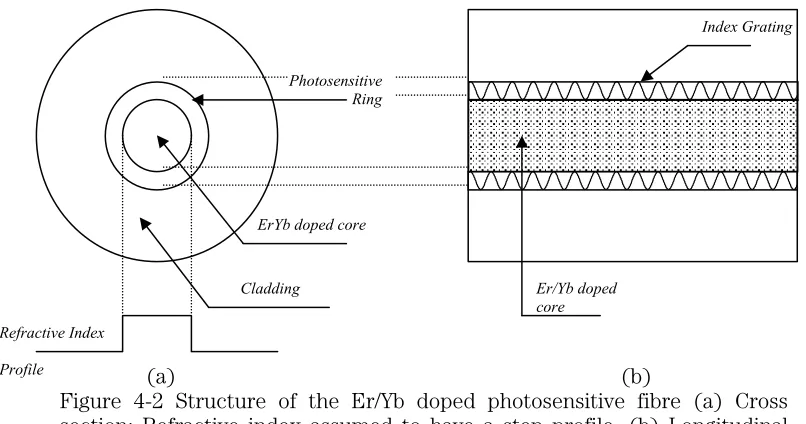
Figure 4-1

shows

these transitions and Table 4-1 details the mechanisms behind them. Also, in reality the

cross-sections vary with temperature [19, 20] . In our model we neglect this effect for the

sake of simplicity. Here N1 is the concentration of the Er ions at 4I15/2 level. An ion at this

energy level is indicated by Er1 in Table 4-1 below. Similarly N2 stands for the

concentration at 4_I

13/2, N3 4I11/2, N4 2H11/2 and 4S3/2 together. For Yb ions N5 is the

concentration at 2_F

Design method for ultimate efficiency in linear cavity continuous wave lasers using distributed feedback

ePrints Soton

from the copyright holder/s. The content must not be changed in any way or sold

of the University School or Department, PhD Thesis, pagination

DESIGN METHOD FOR ULTIMATE EFFICIENCY IN LINEAR-CAVITY CONTINOUS-WAVE LASERS

TABLE OF CONTENTS

CHAPTER 1 INTRODUCTION...10

3.3.SIMULATION OF ACTIVE MEDIUM...31

4.5.FITTING PARAMETERS...51

6.1.INTRODUCTION...75

6.6.CONCLUSIONS...107

7.3.CONCLUSIONS...132

8.4.ALTERNATIVE WAVELENGTHS...147

List of Abbreviations

Meter

cross-section

Energy transfer coefficient between Er

Absorbed pump power per unit length

energy

conversion

any stubborn person can complete a PhD. However, enjoying the entire PhD

to make your postgraduate life enjoyable. With the wisdom of hindsight, I can see

is fantastic. But making things actually work in reality is even more satisfying.

writers’ cramp

1.2. Approach

1.3. Modelling and Simulations

1.4. Overview of the Thesis

1.5. References

2.1. Historical Perspective

2.2. Applications

2.3. References

3.1. Introduction

3.2. Simulation of Propagation in Grating Structures

0

3.3. Simulation of Active Medium

3.4. Conclusions

3.5. References

4.1. Introduction

4.2. Characterisation of Active Medium

Figure 4-1