Dependent Gaussian mixture models for source separation

R E S E A R C H

Open Access

Dependent Gaussian mixture models for

source separation

Alicia Quir ´os

and Simon P Wilson

Abstract

Source separation is a common task in signal processing and is often analogous to factor analysis. In this study, we look at a factor analysis model for source separation of multi-spectral image data where prior information about the sources and their dependencies is quantified as a multivariate Gaussian mixture model with an unknown number of factors. Variational Bayes techniques for model parameter estimation are used. The development of this methodology is motivated by the need to bring an efficient solution to the separation of components in the microwave radiation maps that are being obtained by the satellite mission Planck which has the objective of uncovering cosmic

microwave background radiation. The proposed algorithm successfully incorporates a rich variety of prior information available to us in this problem in contrast to many previous solutions that assume completely blind separation of the sources. Results on realistic simulations of Planck maps and on Wilkinson microwave anisotropy probe fifth year images are shown. The technique suggested is easily applicable to other source separation applications by modifying some of the priors.

Keywords: CMB, Gaussian mixture priors, Variational Bayes

Introduction

The discovery of the cosmic microwave background (CMB) is a strong evidence for the Big Bang theory of the formation and development of the universe. Accord-ing to the theory, the early universe was smaller and hotter but cooled as it expanded. Once the temperature cooled to about 3000 K, photons were free to propagate with-out being scattered off ionized matter; the CMB is an image of this event and is visible across the entire sky. Three satellites have been launched to measure the CMB: the cosmic background explorer, Wilkinson microwave anisotropy probe (WMAP) and most recently the Planck surveyor. Planck is the highest resolution data to date, of the order of 107pixels across the sky measured at nine channels.

Unfortunately, the signals measured by these satellites as shown in Figure 1 contain radiation not only from CMB, but also contributions from a number of other sources, namely foreground radiations and extragalactic sources in addition to antenna receiver noise. Foreground sources

*Correspondence: [email protected]

1Department of Signal Theory and Communications, Universidad Rey Juan Carlos, C° Molino s/n, Fuenlabrada, Madrid, Spain

Full list of author information is available at the end of the article

from our galaxy include synchrotron, dust, and free–free emission. Therefore, the separation of the CMB signal from other sources is an important stage in the production of CMB maps [1].

To date, there have been several attempts to achieve it in a Bayesian framework using both (a) Gaussian mixture model (GMM) prior [3], and (b) Markov Random Field (MRF) prior [4,5]. Full sky maps at low resolution through MCMC, using masks to reduce the effect of the signal in the galactic plane, were described in [6]. Some of these are fully Bayesian source separation methods which are devel-oped to separate the underlying CMB from the mixed observed signals of extraterrestrial microwaves made at several frequencies.

A common assumption among works in the litera-ture is the independence of the cosmological sources. Although it is well known that CMB is independent from the rest of the sources, the galactic sources demonstrate significant statistical dependence among themselves, as stated in [1]. Recently, a small number of researchers have started addressing this problem [7,8]. Various depen-dent component analysis approaches are compared in [9], demonstrating their superior performance with respect to classical ICA.

(a)

(b)

(c)

(d)

(e)

Figure 1Observed WMAP 7 year-data.The data were taken from the NASA WMAP website [2].

In this study, we present a dependent components model for source separation of multi-spectral image data, where prior information about the sources and between-source dependencies is quantified as a multivariate GMM, using variational Bayes techniques for model parame-ter estimation. This article can thus be considered as an extension of [3], modeling dependencies between-sources through generalizing the prior to multivariate GMM.

The rest of the article is structured as follows. The next section gives the model for the mixing problem and describes the hierarchical Bayesian model that we use, including the prior we assume for the sources. Section “Implementing the source separation” describes the vari-ational Bayes approach we use for the implementation of the separation. Section “Examples” provides results on both synthetic Planck and real WMAP images. Finally, we provide a discussion of the results in the last section.

Model

The model description is defined in terms of the microwave source separation problem, where there arenf maps of the sky at frequencies(ν1,. . .,νnf), each map

con-sisting of J pixels. The data are denoteddj ∈ Rnf,j = 1,. . .,J. The source model consists of ns sources and is represented by the vectorssj ∈ Rns, with each compo-nent representing the amplitude of a physical source of microwaves. We assume that thedjcan be represented as a linear combination of thesj:

dj=Asj+ej, (1)

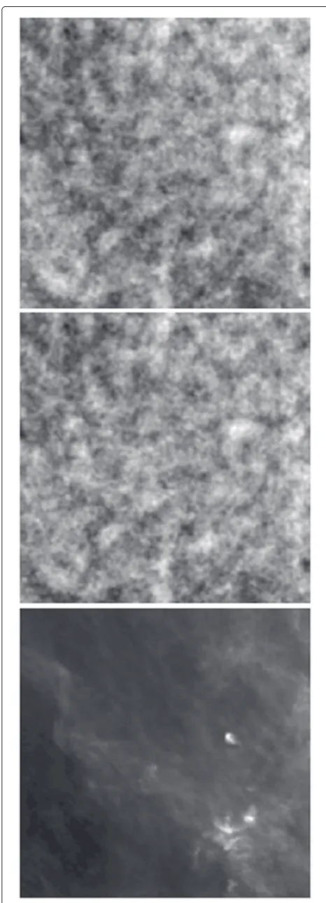
Figure 2Observations on the three of the nine channels (lowest, middle, and highest frequencies are shown) of the data generated from the source separation model with realistic simulations of CMB, synchrotron, and galactic dust.

define

D = {dij|i=1,. . .,nf,j=1,. . .,J}; S = {skj|k=1,. . .,ns,j=1,. . .,J}

to represent all data and sources.

We assume dependence between the sources, defined by a prior distributionp(S|ψ )with parametersψ. The goal is to estimate theSand the parametersψassociated with the model forS, given observation ofD. The noise

vari-ances τ and the mixing matrix A are assumed known.

GMM are used to represent the non-Gaussian sources, in which case it is an example of a model known as a mixture of factor analyzers [10]. As in [10], we adopt a Bayesian approach to the data fitting, implemented by a variational Bayes approach.

Bayesian inference will be based on the posterior dis-tribution, which following the above description can be factorized as

p(S,ψ|A,D,τ )∝p(D|S,A,τ )p(S|ψ )p(ψ ). (2)

Each element of this distribution is defined next in turn.

Noise structure

Gaussian error, ej, is assumed independent within and between pixelsjand frequency, which gives

p(D|S,A,τ )= J

j=1 nf

i=1

τi 2πexp

−τi

2(dij−Ai·sj) 2

(3)

whereAi·is theith row ofA.

Mixing matrix structure

In this application,Ais parameterized and denotedA(θ ). Each column ofA(θ )is the contribution to the observa-tion of a source at different frequencies, which is written as a function of the frequencies andθ. These parameter-izations are approximations that come from the current state of knowledge about how the sources are generated. Here, we merely state the parameterization that we are going to use, and refer to [11] for a more detailed expo-sition on the background to them. Some restrictions are usually placed onA(θ )in order to force a unique solution; this is achieved here by setting the first row ofA(θ )to be ones.

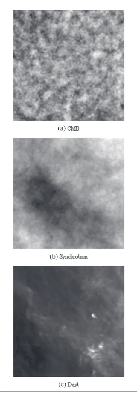
Figure 3The simulated sources used to generate the simulated data in Figure 2.

modeled as a black body at a temperature, and its con-tribution is a known constant at each frequency. The parametrization of the mixing matrix is given as

Ai1(θ )= g(νi) g(ν1)

, (4)

where

g(νi)=

hνi kBT0

2 _exp(hν

i/kBT0) (exp(hνi/kBT0)−1)2

,

T0 = 2.725 K is the average CMB temperature,his the Planck constant, andkBis Boltzmann’s constant. The ratio g(νi)/g(ν1)is designed to ensure thatA11(θ ) = 1 as we constraint the first row ofA(θ )to be ones.

Ai2(θ ) =

νi ν1

κs

,

Ai3(θ ) =

exp(hν1/kBT1)−1 exp(hνi/kBT1)−1

νi ν1

1+κd

, and

Ai4(θ ) =

νi ν₁

κf

,

whereT1=18.1 K is the assumed thermodynamical tem-perature of the dust grains, and column 2 corresponds to synchrotron, column 3 to galactic dust, and column 4 is free–free emission. There are three unknown model parameters forA, for synchrotronκs ∈ {κs :−3.0≤κs ≤

−2.3}, the spectral indices for dustκd ∈ {κd : 1≤κd≤2}, and for free–free emissionκf ∈ {κf :−2.3≤κf ≤ −2.0}.

The sources

The distribution of sj is modeled as a GMM with m

factors. The model proposed allows for between-source dependence; the vector of sources at a pixel is a mixture of multivariate Gaussians

p(S|ψ )= J

j=1 m

a=1

wap(sj|μa,Qa) (5)

where

p(sj|μa,Qa)= | Qa| (2π )ns exp

−1

2(sj−μa) T_Q

a(sj−μa)

Priors

The remaining term in Equation (2) is p(ψ ). We use

the conjugate prior distributions [12] that facilitate the computation of the posterior and yet flexible enough to incorporate good prior information: Gaussians for the component means, Dirichlet for the component weights, and Wishart for precision matrices. In the microwave source application, background knowledge about the magnitude of the sources can be incorporated through specifying values of the parameters of these prior distri-butions. This prior specification follows [13], who discuss how to specify these values in more detail.

Implementing the source separation

The posterior developed in the previous section does not lend itself to an analytical solution. MCMC techniques are one approach that let us evaluate complicated inte-grals by sampling rather than by analytical or numerical methods. The main criticism of Bayesian source sepa-ration with sampling methods, MCMC in particular, is their computational load and slow convergence. Regard-ing the speed, they cannot compete with methods such as FastICA [14,15].

There are several approaches to speed up the algorithm, such as the strategies suggested in [16]. In the image source separation problem framework, the Langevin sam-pling scheme has been implemented [4], as a way to obtain a faster MC algorithm.

In this study, the source separation model presented in Section “Model” is implemented by a variational Bayesian approach [10,17,18], that allows for more effi-cient inference when dealing with large data when com-pared with MCMC techniques. In essence, given the

data D and a model with parameters θ and latent

variables Z, the variational Bayes method is based on approximating the posterior distribution p(Z,θ|D) with a factorial approximation q(Z,θ|φ) = q(Z|φZ)q(θ|φθ),

where φ are the variational parameters. The

approx-imation is fitted by minimizing the Kullback–Leibler divergence between q and p, or equivalently maximiz-ing a lower bound on marginal log-likelihood of the data.

Attias [19] has recently developed a fully Bayesian approach to GMM with a variational approximation to the posterior that, when choosing conjugate priors, leads to the following components: Wishart densities for the precisions,Qa; Normal densities for the means,μa; and a Dirichlet for the mixing coefficients, p; and a dis-crete distribution for the indicator posteriors, zj, which indicates the component that explains information in pixel j. We further derived the variational approxima-tion to the marginal posterior of sources, sj, which turns out to be a multivariate Gaussian distribution. In brief

q(sj) ∼ MVN(Aj,Bj) q(p) ∼ D(λ)

q(μa|Qa) ∼ N(ξa,βaQa) q(Qa) ∼ W(ηa,Va)

and

q(zj=a)∝exp

(λa)−

a

λa

|Va| 1 2₂ns2

exp 1 2 ns i=1

ηa+1−i

2

exp

− ns

2βa

exp−ηa 2

(A_j −ξa)TVa(Aj −ξa)+tr(Va(Bj)−1)

whereMVN stands for multivariate normal distribution and denotes the digamma function. Note thatq(zj = a)is the probability that componentais responsible for information in pixeljin sources,sj.

The quantities of interest, i.e., the hyper-parameters to be computed,A_j,B_j,λ,ξa,βa,ηa, andVaforj= 1,. . .,J anda=1,. . .,m, have the following values:

(B_j)kl = nf

i=1

τiAikAil+ m

a=1

q(zj=a)ηa(Va)kl

(A_j)k = (Bj)−1v(k), with

v(k) = nf

i=1

τ_idijAik+ m

a=1

q(zj=a)ηa ns

l=1

(Va)kl(ξa)l

λa =

j

q(zj=a)+λpriora

ξa =

j[q(zj=a)Aj]+β prior a ξaprior

jq(zj=a)+βaprior

βa =

j

q(zj=a)+βaprior

η_a =

j

q(zj=a)+ηpriora

Va =j

q(zj=a)

1−2q(zj=a)

jq(zj=a)

(B_j)−1+

+(A_j − ¯μa)(A_j − ¯μa)T

+Vaprior

+βaprior[

jq(zj=a)][+(μ¯a−ξaprior)(μ¯a−ξaprior)T

Figure 4The posterior mean of the reconstruction of the CMB with a scatter plot of true versus posterior mean.

with

¯

μ_a =

j[q(zj=a)A_j]

jq(zj=a)

()_kl =

j{[q(zj=a)]2(Bj)−kl1} [_jq(zj=a)]2

.

Computations were carried out using Matlab.

Examples

Analysis of simulated data

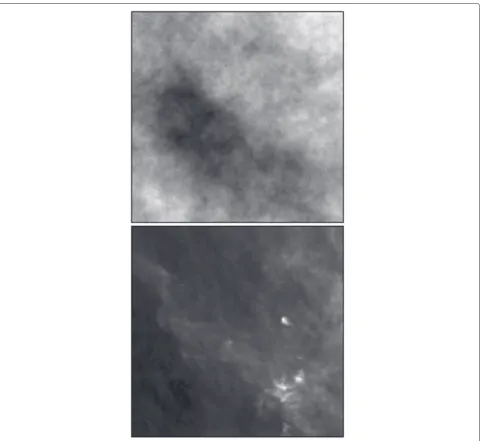
Figure 5The posterior mean of the reconstruction of synchrotron and galactic dust.

by Planck from 30 to 857 GHz. The mixing matrix used was as defined in Section “Mixing matrix structure” with κ_s = −2.9 and κ_d = 2.0. Noise precisions were those published by the Planck research team [21]. After explor-ing several values form, the number of components in the GMM source model was fixed to bem=1, as it provided the best fit, taking into account the compromise between fit and number of parameters in the model.

Figure 4 shows an estimate of CMB, along with a scat-ter plot of this estimate against the true value, as shown in Figure 3. Such an estimate is the average of the samples obtained for the first column of A , which corresponds to CMB. We see from the scatter plot and from compari-son with Figure 3 that the reconstruction of CMB is very

accurate here. The same is true for the other two sources, as shown in Figure 5.

Table 1 shows the mean of the parameters of the model. Regarding the between-sources dependence struc-ture, posterior estimates of V₁−_k1,k = 2, 3 are approxi-mately 0, suggesting independence between CMB and the other sources, as expected. On the other hand, posterior

Table 1 Mean estimate of parameters for simulated data

ˆ

μ=

⎛ ⎜ ⎜ ⎝

0.020 0.014 0.008

⎞ ⎟ ⎟

⎠ Qˆ=

⎛ ⎜ ⎜ ⎝

4.665 0 0

0 0.006 0.003 0 0.003 0.010

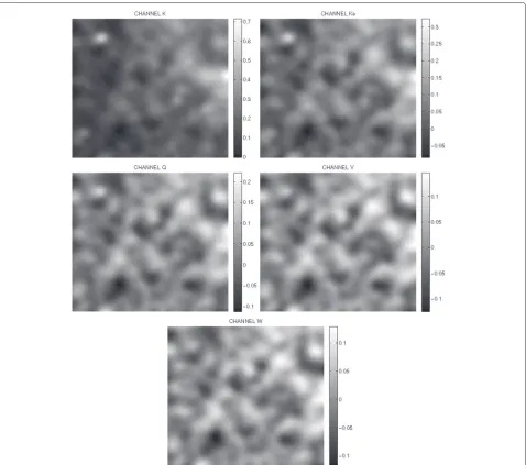
Figure 6Temperatures (in mK) at20◦square patch of the sky from WMAP [2] at 5 microwave frequencies (clockwise from top left) 22, 30, 40, 90, and 60 GHz).

Table 2 Parameter estimated mean for WMAP data

a=1 pˆ1=0.12 μˆ1=

⎛ ⎜ ⎜ ⎜ ⎜ ⎜ ⎝

−0.012 0.051

−0.001 0.017

⎞ ⎟ ⎟ ⎟ ⎟ ⎟ ⎠

ˆ

Q1= ⎛ ⎜ ⎜ ⎜ ⎜ ⎜ ⎝

5.29 0 0 0

0 1.47 ₋0.04 ₋1.60 0 ₋0.04 0.41 0.32 0 ₋1.60 0.32 3.79

⎞ ⎟ ⎟ ⎟ ⎟ ⎟

⎠×

105

a₌2 pˆ2=0.88 μˆ2=

⎛ ⎜ ⎜ ⎜ ⎜ ⎜ ⎝

−0.012 0.029 0.003 0.017

⎞ ⎟ ⎟ ⎟ ⎟ ⎟ ⎠

ˆ

Q2= ⎛ ⎜ ⎜ ⎜ ⎜ ⎜ ⎝

1.45 0 0 0

0 0.54 0.08−0.20 0 0.08 0.28 0.26 0 −0.20 0.26 1.09

⎞ ⎟ ⎟ ⎟ ⎟ ⎟

⎠×

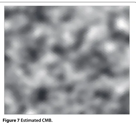
Figure 7Estimated CMB.

estimate of V₂₃−1 = 0, indicating dependence between synchrotron and galactic dust.

Analysis of a WMAP year 5 patch

The WMAP [22] was launched in 2001 and data collection activities finished in 2010. It observes 5 frequencies from 22 to 90 GHz. Figure 6 shows a patch of 5-year WMAP data.

The algorithm was implemented with four sources (CMB, synchrotron, dust, and free–free emission). The noise precisions were assumed to be the published values for WMAP detectors. The spectral density for free–free emission was fixed at−2.14 (following [11]) and the syn-chrotron and dust spectral indices were as in the first example. The number of components in the GMM source

model were fixed to be m = 2, following the same

reasoning as in the simulation study. Informative priors were placed on the GMM parameters, based on discus-sions on the expected marginal properties of the sources. Table 2 shows the mean of the mixture parameters of the model. Figure 7 shows the estimated CMB. The result obtained is in agreement with previous work [3], as can be appreciated in Figure 8 that shows an histogram of the dif-ferences between the estimated CMB using the approach presented here and the estimated CMB obtained in [3].

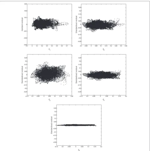
Finally, in order to show the fit of the data to the model, Figure 9 is a scatter plot of the observed value of thedjk with the standardized residuals, with one figure for each frequencyk=1,. . ., 5.

Conclusion

A fully Bayesian factor analysis algorithm has been pre-sented and applied to a multi-channel image source sepa-ration problem, where dependencies between sources are

modeled as a multivariate GMM. The algorithm performs very well on simulated Planck data and has been applied to data from WMAP.

In this study, we extend previous approaches [3] by allowing the source priors to be a mixture of multivariate Gaussian distributions for each pixel.

The development of this methodology is motivated by the need to bring an efficient solution to the separa-tion of components in the microwave radiasepara-tion maps to be obtained by the satellite mission Planck which has the objective of uncovering CMB radiation. The pro-posed algorithm successfully incorporates a rich vari-ety of prior information available to us in this problem in contrast to most of the previous work that assumes completely blind separation of the sources. Further, the variational approach presented here overcomes the con-vergence problems of the MCMC stated in [23], when dealing with large datasets such as that will be provided by the satellite mission Planck.

In the analysis of simulated data, the number of

compo-nents in the GMM source model turned out to bem =

1. This means that sources are multivariate Gaussian a priori. On the other hand, for real data, the number of components ism=2. In blind source separation problem, identifiability relies on the independence of the sources. In this study, in spite of modeling the sources as Gaus-sians whenm = 1, identifiability is obtained because of the prior information which is incorporated to the model, given structure to the mixing matrix.

Another type of dependence is that a source is spa-tially correlated. Spatial dependence is most conveniently

−0.1 0 0.1

Figure 9Assessment of model fit.Scatter plot of the posterior predicted values ofdjagainst the standardized residual over all pixels.

modeled by a Gaussian MRF and some preliminary work on this idea can be found in [5]. Combining with cross source correlations, one might ultimately consider a mix-ture of multivariate Gaussian MRF as a prior for the sources. Implementing the analysis with such a prior would be a significant challenge computationally; we hypothesize that it will be difficult to derive a well-behaved MCMC approach. Other functional approxima-tions, such as that of [24], offer feasible alternative to computing the posterior distribution in this case.

Finally, although the technique was developed for the astrophysical source separation problem in mind, it is general and it is applicable to other source separation problems as well.

Competing interests

Both authors declare that they have no competing interests.

Acknowledgements

08/IN.1/I1879. The authors acknowledge the use of the PSM, developed by the Component Separation Working Group (WG2) of the Planck Collaboration.

Author details

1_{Department of Signal Theory and Communications, Universidad Rey Juan}

Carlos, C° Molino s/n, Fuenlabrada, Madrid, Spain.2_{Department of Statistics,}

Trinity College Dublin, Dublin 2, Ireland.

Received: 31 January 2012 Accepted: 30 October 2012 Published: 16 November 2012

References

1. EE Kuruoglu, Bayesian source separation for cosmology. IEEE Signal Process. Mag.27, 43–54 (2010)

2. http://lambda.gsfc.nasa.gov/product/map/current/m products.cfm 3. SP Wilson, EE Kuruoglu, E Salerno, Fully Bayesian source separation of

astrophysical images modelled by a mixture of Gaussians. IEEE J. Sel. Topics Signal Process.2(5), 685–696 (2008)

4. K Kayabol, EE Kuruoglu, JL Sanz, B Sankur, E Salerno, D Herranz, Adaptive Langevin sampler for separation of t-distribution modelled astrophysical maps. IEEE Trans. Image Process.19(9), 2357–2368 (2010)

5. K Kayabol, EE Kuruoglu, B Sankur, Bayesian separation of images modeled with MRFs using MCMC. IEEE Trans. Image Process.18(5), 982–994 (2009) 6. C Dickinson, HK Eriksen, AJ Banday, JB Jewell, KM Gorski, G Huey, CR

Lawrence, IJ O’Dwyer, BD Wandelt, Bayesian component and separation cosmic microwave background estimation for the five-year WMAP temperature data. Astrophys. J.705, 1607–1623 (2010)

7. L Bedini, D Herranz, E Salerno, C Baccigalupi, EE Kuruoglu, A Tonazzini, Separation of correlated astrophysical sources using multiple-lag data covariance matrices. EURASIP J. Appl. Signal Process.2005(15), 2400–2412 (2005)

8. A Bonaldi, L Bedini, E Salerno, C Baccigalupi, G De Zott, Estimating the spectral indices of correlated astrophysical foregrounds by a second-order statistical approach. Monthly Notices R. Astron. Soc.373, 271–279 (2006) 9. EE Kuruoglu, Dependent component analysis for cosmology. Lecture

Notes Comput. Sci.6365, 538–545 (2010)

10. Z Ghahramani, M Beal, inAdvances in Neural Information Processing Systems, ed. by SA Solla, TK Leen, and KR Muller. Variational inference for Bayesian mixtures of factor analysers (MIT Press, Cambridge, MA), 2000) 11. HK Eriksen, C Dickinson, CR Lawrence, C Baccigalupi, AJ Banday, KM Gorski,

FK Hansen, PB Lilje, E Pierpaoli, KM Smith, K Vanderlinde, C M B component separation by parameter estimation. Astrophys. J.641, 665–682 (2006) 12. PM Lee,Bayesian Statistics: An Introduction, 3rd edn. (Hodder Arnold H& S,

London, 2004)

13. S Richardson, P Green, On Bayesian analysis of mixtures with an unknown number of components (with discussion). J. R. Stat. Soc. Ser. B.59, 731–792 (1997)

14. A Hyv¨arinen, Fast and robust fixed-point algorithms for independent component analysis. IEEE Trans. Neural Netw.10(3), 626–634 (1999) 15. S Leach, JF Cardoso, C Baccigalupi, R Barreiro, M Betoule, J Bobin, A

Bonaldi, J Delabrouille, G De Zotti, C Dickinson, HK Eriksen, J

Gonz´alez-Nuevo, FK Hansen, D Herranz, M Le Jeune, M L ´opez-Caniego, E Mart´ınez-Gonz´alez, M Massardi, JB Melin, MA Miville-Desch ˆenes, G Patanchon, S Prunet, S Ricciardi, E Salerno, JL Sanz, JL Starck, F Stivoli, V Stolyarov, R Stompor, P Vielva, Component separation methods for the PLANCK mission. Astron. Astrophys.491(2), 597–615 (2008)

16. WR Gilks, S Richardson, DJ Spiegelhalter,Markov Chain Monte Carlo in Practice. (CRC Press, Boca Raton, FL, 1996)

17. DJC McKay,Information Theory, Inference and Learning Algorithms. (Cambridge University Press, Cambridge, 2003)

18. CM Bishop,Pattern Recognition and Machine Learning. (Springer, New York, 2006)

19. H Attias,A Variational Bayesian Framework for Graphical Models. (MIT Press, Cambridge, MA, 2000)

20. P Collaboration, The pre-launch plack sky model: a model of sky emission at submillimetre to centimetre wavelengths (in preparation)

21. http://sci.esa.int/science-e/www/object/index.cfm?fobjectid=34730& fbodylongid=1595

22. http://map.gsfc.nasa.gov/

23. SP Wilson, EE Kuruoglu, A Quir ´os, in2nd International Workshop on Cognitive Information Processing. Bayesian factor analysis using Gaussian

mixture sources, with application to separation of the cosmic microwave background, (2010), pp. 198–202

24. H Rue, S Martino, N Chopin, Approximate Bayesian inference for latent Gaussian models using integrated nested Laplace approximations. J. R. Stat. Soc. Ser. B.71, 319–392 (2008)

doi:10.1186/1687-6180-2012-239

Cite this article as:Quir ´os and Wilson:Dependent Gaussian mixture models for source separation.EURASIP Journal on Advances in Signal Processing2012

2012:239.

Submit your manuscript to a

journal and benefi t from:

7Convenient online submission

7 Rigorous peer review

7Immediate publication on acceptance

7 Open access: articles freely available online

7High visibility within the fi eld

7 Retaining the copyright to your article