Design of an active compliant liquid column damper by LQR and wavelet linear quadratic regulator control strategies

(1)

Design of an Active Compliant Liquid Column Damper by LQR and Wavelet LQR Control Strategies

Soumi Bhattacharyya1_{, Aparna (Dey) Ghosh}2_{, Biswajit Basu}3

1_{Research Scholar, Department of Civil Engineering, Indian Institute of Engineering Science and}

Technology, Shibpur, Howrah-711103, India. email: [email protected]

2_{Professor, Department of Civil Engineering, Indian Institute of Engineering Science and}

Technology, Shibpur, Howrah-711103, India. email: [email protected], [email protected]

3_{Professor, Department of Civil, Structural and Environmental Engineering, Trinity College}

Dublin, Ireland. email: [email protected]

(2)

Keywords: Compliant liquid column damper (CLCD), LQR algorithm, wavelet LQR algorithm, active control, seismic vibration control, time domain study

Introduction

The Tuned Liquid Column Damper (TLCD) was first proposed by Saoka et al.[1]_{and Sakai}_et

al.[2]_{as a passive control device for structures. Since then, considerable research has been carried}

out on the device for the mitigation of wind-induced vibration[3-7]_{as well as for seismic vibration}

control of flexible structures[8-13]_{. The TLCD offers several advantages as compared to the tuned}

sloshing damper such as high volumetric efficiency with respect to a given amount of liquid, consistent behaviour across a wide range of excitation levels and a damping mechanism that can be quantified in a definite manner. Some prominent TLCD implementations are in the Higashi-Kobe cable-stayed bridge in Japan[14]_{, the 106.2 m high Hotel Cosima in Tokyo}[15]_{and the 194.4}

m high Shin Yokohama Prince Hotel in Japan[16]_{. In the TLCD, the frequency of oscillation of}

the liquid is dependent only on the total length of the liquid column, thereby rendering the TLCD a long period system. This generally restricts its direct application to the vibration control of structures with fundamental frequencies above 0.5 Hz[17]_{. To extend the applicability of the}

passive TLCD to the short period range, several modifications to the original TLCD configuration have been proposed. In a sealed TLCD approach, Reiterer and Ziegler[18]_utilized

the air spring effects in a sealed U-tube to extend the applicability of the TLCD to 4.0 to 5.0 Hz. In another approach, Ghosh and Basu[19]_{proposed a compliant model of the TLCD, termed the}

CLCD in subsequent works, in which the U-tube containing the damper liquid is flexibly connected to the structure, providing an additional degree of freedom by which the direct tuning of the oscillating liquid column to the structure is avoided. Ghosh and Basu[20]_{studied the}

robustness of single and multiple CLCDs and carried out a preliminary experimental investigation on the CLCD, results of which indicated the potential of the proposed damper. Ghosh and Basu[13]_{further proposed a design methodology for the spring-connected LCD as a}

seismic vibration control device for structures considering nonlinear behaviour. Gur et al.[21]

replaced the linear spring of the CLCD by a spring made of shape memory alloy for improved performance and robustness. Recently, a detailed experimental verification of the theoretical model of the CLCD was carried out by Bhattacharyya et al.[22]_{. It may be noted that the CLCD,}

(3)

To further improve the efficiency and robustness of the passive TLCD, considerable development in active, semi-active and hybrid control applied to various configurations of the TLCD has taken place. In the active TLCD configurations, researchers have considered various means to apply the control force to the damper and have calculated the control parameters through the use of different control algorithms. In the active TLCD studied by Balendra et al.[23]_,

the TLCD is supported on a movable platform to which the control force, evaluated by the H∞ algorithm, is applied for suppression of wind induced vibrations of a tower. Chen and Ko[24]

proposed installing two propellers inside the TLCD and used feedback optimal control theory to calculate the control force for seismic control. Hochrainer and Ziegler[25]_{actively controlled the}

air spring effect of a sealed TLCD by applying a bang-bang controller on the pressure valve. Haroun et al.[26]_{studied a hybrid TLCD, for vibration mitigation of tall buildings under}

earthquake and wind loading, in which the orifice opening ratio is actively controlled by an optimal control algorithm. A hybrid TLCD system for control of structural response under seismic excitation was studied by Kim and Adeli[27]_{who optimally adjusted the head loss}

coefficient by changing the orifice opening ratio using a wavelet-hybrid feedback least mean square (LMS) control algorithm.

Yalla et al.[28]_{developed clipped-optimal and fuzzy control strategy based semi-active}

algorithms for controlling the orifice opening and investigated the effectiveness of these algorithms for a 5-storied building subjected to wind excitation. Yalla and Kareem[29]_conducted

an experimental study on a semi-active TLCD equipped with an electropneumatic valve utilizing the control strategy based on gain scheduling and further illustrated the performance of the damper for controlling the wind induced vibration of tall buildings through numerical simulations. Li and Huo[30]_{and Li}_{et al.}[31]_{used semi-active neural networks on the TLCD for}

vibration control of irregular buildings. An energy based semi-active control strategy was investigated by Bigdeli and Kim[32]_{for control of irregular structures under seismic excitation.}

Sonmez et al.[33]_{proposed an adaptive spring connection between the TLCD and the structure to}

cater to off-tuning conditions and a short time Fourier transformation (STFT) based controller was designed to control the stiffness of the spring in real time. Several semi-active TLCDs with magnetorheological (MR) fluid as the damper liquid have also been proposed by Ni et al.[34]_,

Wang et al.[35]_{and Colwell and Basu}[36]_{. For recent studies of structural control see discussions}

(4)

In this paper an active configuration of the CLCD (ACLCD) is proposed for control of seismic vibrations of structures. The controller design is first carried out by using the Linear Quadratic Regulator (LQR) algorithm and then subsequently by developing a multiresolution based Wavelet Linear Quadratic Regulator (WLQR) algorithm following Basu and Nagarajaiah[38]_{. The}

design procedure developed for the ACLCD is illustrated both for an example flexible structure as well as for an example stiff structure, subjected to a recorded accelerogram input. As the basic parameters of the ACLCD are based on the optimal design of the corresponding passive CLCD, the results of the latter are first obtained. The optimum control parameters of the ACLCD are then evaluated with the objective of minimizing the displacement response of the structure and satisfying the constraints on peak liquid and whole damper displacements. Further, the structural response reductions achieved by the ACLCD are studied while varying the values of the controller parameters and the stability of response reduction is considered to be maintained till the point where the gradient of the response reduction curve becomes discontinuous. The performances of the LQR and WLQR based control strategies are compared, in terms of both structural response reduction and requirement of peak control force magnitudes, through a detailed time domain study. The tolerance of the control strategies against variability in excitation is also studied.

Modelling and equations of motion for structure-ACLCD system

The mathematical model of the proposed ACLCD, incorporated into a SDOF structural system, subjected to the horizontal ground acceleration, 𝑧̈(𝑡), is shown in Fig. 1. 𝑚 represents the mass of the structure having a stiffness of 𝑘𝑠 and a damping of 𝑐𝑠. 𝑘2 is the stiffness of the spring connected to the damper. 𝐵 and 𝐿 represent the horizontal and total length of liquid column.

𝑥(𝑡), 𝑦(𝑡) and 𝑢(𝑡) represent the displacements of structure, whole damper system and damper liquid respectively. These responses are measured by sensors located appropriately as shown in Fig. 1. Based on the feedback from the sensors, the controller generates the force signal and the required control force is applied by the actuator to the damper container.

The equation of motion for the liquid in the CLCD is given by

𝜌𝐴𝐿𝑢̈(𝑡) +1

(5)

where, 𝜉 is the orifice head loss coefficient and 𝜌 is the density of the damper liquid. Normalizing Eq. (1) with respect to the liquid mass, 𝜌𝐴𝐿, leads to

𝑢̈(𝑡) + 𝜉

2𝐿|𝑢̇(𝑡)|𝑢̇(𝑡) + 𝜔12𝑢(𝑡) = −𝛼(𝑦̈(𝑡) + 𝑥̈(𝑡) + 𝑧̈(𝑡)) (2)

where, 𝜔1 [= √(2𝑔 ⁄ 𝐿)] is the natural frequency of the oscillating liquid column (commonly termed as the LCD frequency) and 𝛼 = 𝐵/𝐿.

Figure 1

The dynamic equilibrium of the whole damper system leads to the following equation (Eq. (3)), in which the actuator force is denoted by 𝑓(𝑡).

(𝜌𝐴𝐿 + 𝑀_𝑐)(𝑦̈(𝑡) + 𝑥̈(𝑡) + 𝑧̈(𝑡)) + 𝜌𝐴𝐵𝑢̈(𝑡) + 𝑘₂𝑦(𝑡) = 𝑓(𝑡) (3)

Normalization of Eq. (3) with respect to (𝜌𝐴𝐿 + 𝑀_𝑐) yields

(𝑦̈(𝑡) + 𝑥̈(𝑡) + 𝑧̈(𝑡)) + 𝛼

1 + 𝜏𝑢̈(𝑡) + 𝜔22𝑦(𝑡) =

𝑓(𝑡)

(𝜌𝐴𝐿 + 𝑀𝑐) (4)

where, 𝜔₂ [= √(𝑘₂⁄ (𝜌𝐴𝐿 + 𝑀_𝑐))], is the natural frequency of the whole damper system and

𝜏 [= 𝑀_𝑐⁄𝜌𝐴𝐿], is the ratio of the container mass to the liquid mass.

The equation of motion for the SDOF structural system, normalized w.r.t the mass, 𝑚, is given by

(𝑥̈(𝑡) + 𝑧̈(𝑡)) + 2𝜁𝑠𝜔𝑠𝑥̇(𝑡) + 𝜔𝑠2𝑥(𝑡) = 𝜇𝜔22𝑦(𝑡) −

𝑓(𝑡)

𝑚 (5)

where, 𝜔_𝑠 is the natural frequency of structure, 𝜁_𝑠 is the damping ratio of the structure and 𝜇 is the ratio of the CLCD mass to the structural mass.

Now, by adopting an equivalent linearization procedure, Eq. (1) may be written as

𝜌𝐴𝐿𝑢̈(𝑡) + 2𝜌𝐴𝐶𝑝𝑢̇(𝑡) + 2𝜌𝐴𝑢(𝑡)𝑔 = −𝜌𝐴𝐵(𝑥̈(𝑡) + 𝑦̈(𝑡) + 𝑧̈(𝑡)) (6)

(6)

controllers are designed for random input, the following expression between 𝐶𝑝 and 𝜉 [3] is considered,

𝐶_𝑝 = 𝜉𝜎𝑢̇

√2𝜋 (7)

where, 𝜎𝑢̇ is the standard deviation of the liquid velocity 𝑢̇(𝑡). Description of example structural systems and input data

Two example SDOF structural systems, one relatively flexible and the other stiff, termed as 𝑆1

and 𝑆2, are considered. The former is the fundamental mode representation of a 81 m tall tower of mass 106_{kg, with a time period of 2.04 s and 1 % damping ratio}[23]_{while a SDOF system of}

the same mass and damping but of 0.5 s time period is taken as the stiff structure[19]_{. The design}

of the ACLCD is carried out for these structures considering them to be subjected to the recorded accelerogram of the S00E component of the 1940 Imperial Valley earthquake at El Centro site with peak ground acceleration (PGA) of 0.348 g. The ACLCD performances are further examined under five more base motions, namely the N85E component of the 1966 Parkfield, California earthquake (station 1014 Cholame #5, Shandon) with PGA of 0.442 g, the SE component of the 1952 Kern County earthquake (station Taft, CA - Lincoln School-810N Sixth) with PGA of 0.179 g, the N05W component of 1991 Uttarkashi earthquake (station Bhatwari) with PGA of 0.247 g, the N10W component of 1999 Chamoli - NW Himalaya earthquake (station Joshimath) with PGA of 0.064 g scaled up by a factor of three and the 1980 Mammoth Lakes, California earthquake (station 54099, SMA-1 S/N 2593) with PGA of 0.180 g. It may be noted that all six earthquake ground motions have similar energy content and not widely varying PGA values. Further, the natural frequencies of S1 and S2 lie in the dominant frequency range of all the input ground motions.

Design and performance of passive CLCD

(7)

practical constraints on peak whole damper displacements, here an arbitrarily selected value of 1 m (𝑦_𝑙𝑖𝑚) is taken as the limiting value of the peak whole damper displacement.

The optimum tuning ratios (𝜈_𝑜𝑝𝑡) and optimum head loss coefficients (𝜉_𝑜𝑝𝑡) of the passive CLCDs are obtained by solving the constrained optimization problem with the objective of minimizing the peak structural displacement. The other damper parameters such as 𝜇, 𝜏, 𝛼 are assumed constant and realistic and feasible values are selected for the same. In the present study, a mass ratio (𝜇) of 2 %, container mass to liquid mass ratio (𝜏) equal to 0.5, and length ratios (𝛼)

of 0.4 and 0.7 are considered. In all, four CLCDs are designed for 𝑆1 and 𝑆2, which are designated as 𝑆𝑖 − 𝑘 (𝑖 = 1, 2; 𝑘 = 1, 2) considering 𝛼 equal to 0.4 and 0.7 respectively.

In case of the stiff structure (𝑆2), it is assumed that the length of the liquid column (𝐿) is constant and equal to 2 m while the frequency of the whole damper system is tuned to the structural frequency. Thus, the tuning ratio is defined by the ratio 𝜔₂⁄𝜔_𝑠. However, in case of the flexible structure (𝑆1), a new approach for tuning is required as so far the CLCD has been studied for stiff structures, the frequencies of which cannot be directly tuned to the oscillating liquid column frequency. Here, the following approach is proposed in which it is assumed that the uncoupled frequencies of the oscillating liquid column (𝜔1) and whole damper motion (𝜔2) are equal (= 𝜔𝑐 say) and that the first coupled frequency of the CLCD (𝜔₁′′_{), from Ghosh and Basu}[13]_{, is tuned}

to the natural frequency of the structure (𝜔_𝑠) at the considered tuning ratio (𝜈 = 𝜔₁′′ _𝜔 𝑠

⁄ ). By this, the value of 𝜔𝑐 is obtained. Thereby, the length of liquid column (𝐿) is obtained from 𝜔𝑐 =

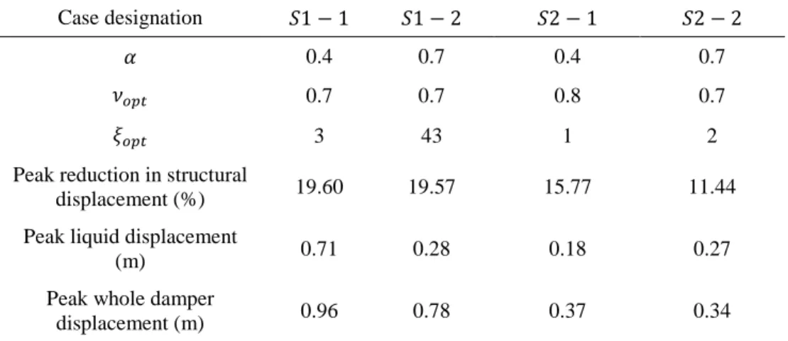
𝜔₁ = √2𝑔 𝐿⁄ . It is thus to be noted that in the design of the CLCD for a flexible structure, 𝐿 is not chosen arbitrarily as in case of the stiff structure, but is dependent on the value of tuning ratio, similar to the conventional TLCD. In the present case, the values of 𝐿 for 𝑆1 − 1 and 𝑆1 − 2 are obtained as 2.44 m and 2.69 m respectively. The optimal values of the passive damper parameters along with the peak reductions in structural displacement and corresponding peak liquid and whole damper displacements are presented in Table 1.

Further, the sensitivity of the response reduction achieved by the passive CLCDs to 𝜉 and the effect of the constraints on the selection of 𝜉_𝑜𝑝𝑡 are examined to later compare with that of the ACLCD. The displacement response reductions of 𝑆1 and 𝑆2 for varying 𝜉, at the values of 𝜈_𝑜𝑝𝑡

(8)

displacement plots are in Figs. 3 and 4 respectively, in which the maximum allowable values are indicated.

Figure 2 Figure 3 Figure 4

It is observed from Fig. 2 that the passive CLCD performance in case 𝑆1 − 1 is sharply sensitive to the variation of 𝜉, whereas for case 𝑆1 − 2, the performance remains consistent beyond the optimum value. Fig. 2 also indicates that both in cases 𝑆2 − 1 and 𝑆2 − 2, the passive damper performances are insensitive to the variation of 𝜉. An inspection of Figs. 3 and 4 reveal that for cases 𝑆1 − 1 and 𝑆2 − 2 the values of 𝜉𝑜𝑝𝑡 are constrained optimum whereas for cases 𝑆1 − 2 and 𝑆2 − 1 the constraints are not active.

The uncontrolled and passive CLCD controlled time histories of the structural displacement for

𝑆1 and 𝑆2 are shown in Figs. 5a and 5b respectively. Figure 5 Design of ACLCD by LQR algorithm

First, the design of the controller is carried out by the LQR algorithm. As the CLCD is an inherently nonlinear system due to the nature of the orifice damping, an equivalent linearized structure-ACLCD system is obtained through stochastic linearization in order to evaluate the gain matrix, which is then multiplied by the response of the nonlinear structure-ACLCD system to obtain the actuator control force. It is to be noted that as the LQR is a classical control technique, the geometrical constraints are explicitly checked and not handled in the derivation of the controller.

LQR control formulation

The dynamical system shown in Fig. 1 can be represented in state-space matrix form as

{𝑋̇} = [𝐴]{𝑋} + [𝐵]{𝑈} + {𝐹} (8)

(9)

[𝐴] =

[

0 1 0 0 0 0

−𝜔_𝑠2 _−2𝜁

𝑠𝜔𝑠 𝜇𝜔22 0 0 0

0 0 0 1 0 0

𝜔𝑠2 2𝜁𝑠𝜔𝑠 −𝜔22 1+𝜏+𝛿𝜇_𝛿 0 𝛼𝜔1

2

𝛿

𝛼 𝛿

2𝐶𝑝

𝐿

0 0 0 0 0 1

0 0 𝛼𝜔₂2 1+𝜏

𝛿 0 −𝜔12 1+𝜏𝛿 − 1+𝜏

𝛿 2𝐶𝑝

𝐿 ]

(9)

where, 𝛿 = 1 + 𝜏 − 𝛼2_.

The control influence matrix is given by

[𝐵] = [0 _𝑚1 0 1+𝜏+𝛿𝜇_𝜇𝛿𝑚 0 −𝛼(1+𝜏)_𝜇𝛿𝑚 ]𝑇 (10) The state vector is as follows.

{𝑋} = {𝑥 𝑥̇ 𝑦 𝑦̇ 𝑢 𝑢̇}𝑇₍₁₁₎ In Eq. (8), the input vector is {𝑈} and {𝐹} is the external excitation vector.

As the LQR is an optimal state-feedback controller, the main objective is to maintain the state close to equilibrium while keeping the control effort optimal in terms of the minimal value of the cost function, 𝐽. The state-feedback law is as follows.

{𝑈} = −[𝐺]{𝑋} (12) The optimal gain matrix ([𝐺]) is evaluated such that the state-feedback law minimizes the quadratic cost function defined as follows.

𝐽 = ∫({𝑋}𝑇_{[𝑄]{𝑋} + {𝑈}}𝑇_{[𝑅]{𝑈})} ∞

0

𝑑𝑡 (13)

Here, [𝑄]6×6 is a symmetric positive semi-definite weighting matrix associated with the state vector and [𝑅]1×1 is a strictly positive-definite symmetric weighting matrix associated with the control force.

(10)

Design of LQR controller and ACLCD performance

Considering the El Centro earthquake excitation as the design input, the controller of the ACLCD is designed for the damper parameters as specified for the passive CLCD. The control parameters are evaluated for 𝑆1 and 𝑆2, from the LQR algorithm, and the results of the structural response reductions along with the corresponding control forces are presented. Utilizing the LQR algorithm for the controller design, the optimum weighting matrix, [𝑄], associated with the state

{𝑋}, is determined for a given weighting matrix associated with the applied control force, [𝑅], considering the constraints of liquid and damper displacements.

The minimum value possible to provide for 𝑅 from the consideration of the stability of response reduction is denoted as 𝑅_𝑙𝑖𝑚. The investigation with higher values of 𝑅 is carried out to estimate the control force required to obtain lower response reductions and to provide design options depending upon the possible cost involvement. The 𝑅 value which provides maximum response reduction in the range investigated is denoted as 𝑅𝑜𝑝𝑡. In [𝑄], higher weights are assigned to the terms associated with the structural responses as greater emphasis is placed on response reduction of the structure. The optimum [𝑄] is determined for each considered value of 𝑅. The peak reduction in structural displacement and the corresponding maximum value of control force are noted for each case and the optimum combination of 𝑅 and [𝑄] is chosen based on the highest value of structural response reduction.

The weighting matrix [𝑄] may be expressed as follows.

[𝑄] =

[

𝑞11(𝑆𝑖) 0 0 0 0 0

0 𝑞₂₂(𝑆𝑖) 0 0 0 0

0 0 𝑞₃₃(𝑆𝑖) 0 0 0

0 0 0 𝑞₄₄(𝑆𝑖) 0 0

0 0 0 0 𝑞₅₅(𝑆𝑖) 0

0 0 0 0 0 𝑞₆₆(𝑆𝑖)]

; 𝑖 = 1, 2 (14)

Here, 𝑞₁₁(𝑆𝑖) and 𝑞₂₂(𝑆𝑖) (𝑖 = 1, 2) denote the weights for the structural displacement and velocity responses respectively. Here, equal weights for these responses are assumed, i.e. 𝑞₁₁(𝑆𝑖) = 𝑞₂₂(𝑆𝑖) = 𝑞(𝑆𝑖)₍_{𝑖 = 1, 2}_{). Further in Eq. (14), the elements}_𝑞

(11)

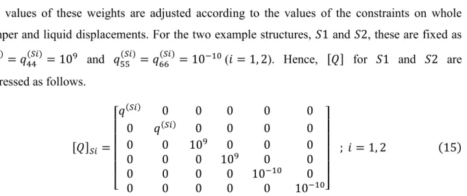
The values of these weights are adjusted according to the values of the constraints on whole damper and liquid displacements. For the two example structures, 𝑆1 and 𝑆2, these are fixed as

𝑞₃₃(𝑆𝑖) = 𝑞₄₄(𝑆𝑖) = 109_and _𝑞

55(𝑆𝑖)= 𝑞66(𝑆𝑖)= 10−10(𝑖 = 1, 2). Hence, [𝑄] for 𝑆1 and 𝑆2 are expressed as follows.

[𝑄]𝑆𝑖 =

[

𝑞(𝑆𝑖) 0 0 0 0 0

0 𝑞(𝑆𝑖) ₀ ₀ ₀ ₀

0 0 109 ₀ ₀ ₀

0 0 0 109 ₀ ₀

0 0 0 0 10−10 ₀

0 0 0 0 0 10−10_]

; 𝑖 = 1, 2 (15)

For each considered value of 𝑅, the weightage on the structural response that provides maximum displacement reduction under the given constraints, denoted by 𝑞_𝑜𝑝𝑡(𝑆𝑖) (𝑖 = 1, 2), is evaluated. The procedure is now illustrated through the design of the controllers for 𝑆1 − 2 and 𝑆2 − 2. In each case 𝑅𝑙𝑖𝑚 = 0.0006. The variations in the peak liquid and whole damper displacements for a range of values of 𝑞(𝑆1)_and_𝑞(𝑆2)_for_{𝑆1 − 2}_and_{𝑆2 − 2}_{, keeping}_{𝑅 = 𝑅}

𝑙𝑖𝑚, are shown in Figs. 6 and 7 respectively.

Figure 6 Figure 7

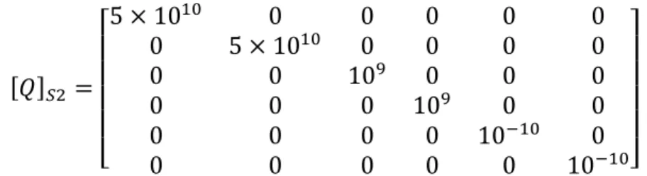
From Figs. 6 and 7 it is observed that the active constraint in each case of 𝑆1 − 2 and 𝑆2 − 2 is that on the peak liquid displacement, which limits the maximum value that may be assigned to

𝑞_𝑜𝑝𝑡(𝑆1) and to 𝑞_𝑜𝑝𝑡(𝑆2) as 4 × 1010_and_{5 × 10}10_{respectively. Hence, the optimum}_[𝑄]_{for the} controller is expressed by

[𝑄]_𝑆1 =

[

4 × 1010 ₀ ₀ ₀ ₀ ₀

0 4 × 1010 ₀ ₀ ₀ ₀

0 0 109 ₀ ₀ ₀

0 0 0 109 ₀ ₀

0 0 0 0 10−10 ₀

0 0 0 0 0 10−10_]

(12)

[𝑄]𝑆2 =

[

5 × 1010 ₀ ₀ ₀ ₀ ₀

0 5 × 1010 ₀ ₀ ₀ ₀

0 0 109 ₀ ₀ ₀

0 0 0 109 ₀ ₀

0 0 0 0 10−10 ₀

0 0 0 0 0 10−10_]

(17)

Figs. 6 and 7 also indicate that, as expected, the peak values of the damper displacements are significantly lower for the stiffer structure, i.e. 𝑆2, as compared to the flexible structure 𝑆1. The resulting time histories of structural displacement and control force (expressed as a percentage of the structural weight) generated by the designed LQR controller, as well as the liquid displacement and whole damper displacement time histories, are presented in Figs. 8 and 9 respectively.

Figure 8 Figure 9

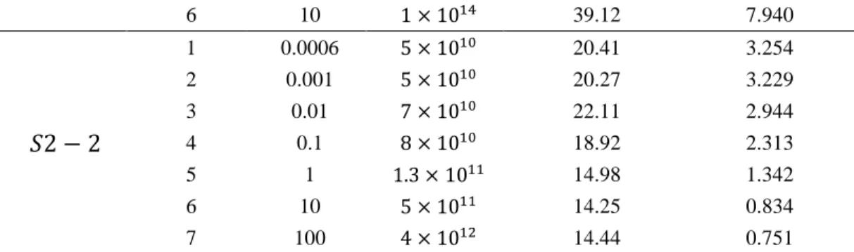
This procedure is repeated for a range of 𝑅 values, 𝑅𝑙𝑖𝑚 to 100, for the cases 𝑆1 − 1, 𝑆1 − 2,

𝑆2 − 1 and 𝑆2 − 2, and the results are presented in Table 2. From this table, on the basis of maximum peak reduction in structural displacement by the ACLCD, the values of 𝑅𝑜𝑝𝑡 are obtained as 0.0004, 0.0006, 0.0005 and 0.01 for cases 𝑆1 − 1, 𝑆1 − 2, 𝑆2 − 1 and 𝑆2 − 2

respectively.

The comparative results of response reductions by the ACLCD and the passive CLCD are presented in Table 3. Here it is clear that considerably higher response reductions are possible by the ACLCD as maximum peak reductions of 27.7 % and 47.09 % are achieved by the ACLCD as against 19.57 % and 15.77 % by the passive CLCD, for the example structures 𝑆1 and 𝑆2

respectively.

(13)

Figure 10

Next, the sensitivity of the controller performance with the head loss coefficient, 𝜉, is investigated. The response reductions achieved by the ACLCD are obtained for a range of 𝜉 for the cases corresponding to 𝑅𝑙𝑖𝑚 in Table 2 and compared with that of the passive CLCD cases in Fig. 11. The value of 𝑞_𝑜𝑝𝑡(𝑆𝑖) (𝑖 = 1, 2) is evaluated for each value of 𝜉. It is observed that in comparison to the passive CLCD, the ACLCD performs better over a wide range of 𝜉 and that the ACLCD performance is insensitive to 𝜉 beyond the optimum value in all the cases. In the design of the passive CLCD for case 𝑆1 − 1, it is clear that 𝜉 greater than 30 cannot be provided whereas the ACLCD provides a consistently good performance over the entire range of 𝜉

studied. Hence, the effective performance of the ACLCD is ensured even in the case of unavailability of optimum 𝜉, as may be due to practical constraints. Thus, in comparison to the passive CLCD, the ACLCD provides flexibility in the choice of 𝜉.

Figure 11

Another point to be noted is that, in case of the flexible structure 𝑆1, the response reduction is not increased beyond 28 % over the considered variation of 𝜉. However, in case of the stiff structure 𝑆2, more than 50 % response reduction could be achieved, which indicates higher effectiveness of the damper for comparatively stiffer structures. From Figs. 11b and 11d, it is also observed that for both types of structures, higher value of 𝛼, i.e. cases 𝑆1 − 2 and 𝑆2 − 2, result in greater sensitivity of the performance of the ACLCD to 𝜉. Further, it is to be noted from Fig. 11d that, unlike in the passive case, in the ACLCD design, response reduction increases with the increase in 𝜉, which reveals that the optimal parameters for passive CLCD, as presented in Table 1, may not always be optimal for the ACLCD.

Performance of designed LQR controller against excitation variability

(14)

in Table 2 for test cases 𝑆1 − 2 and 𝑆2 − 2 respectively are chosen. The gain, [𝐺], is obtained for the El Centro excitation and then the structure is subjected to the other excitations and the control force, {𝑈}, is evaluated by multiplying the structural response with gain [𝐺] (Eq. (12)). The response reductions achieved without violating the constraints and the corresponding required peak control forces are presented in Table 4. From Table 4 it is observed that the LQR controller designed for the structure-ACLCD system subjected to the El Centro earthquake input is also providing a satisfactory performance for the other base excitations. The representative time history results for structural displacement and control force for the flexible (𝑆1 − 2) and stiff (𝑆2 − 2) structures are shown in Figs. 12 and 13 respectively.

Figure 12 Figure 13

Design and performance of ACLCD by WLQR algorithm

Here, a multiresolution based wavelet controller (WLQR), originally proposed by Basu and Nagarajaiah[38]_{, is designed for the ACLCD, with the objective of achieving structural}

displacement response reductions comparable to that obtained from the conventional LQR controller, but by the application of comparatively lower control forces. This is illustrated for some selected combinations of 𝑅 and corresponding 𝑞_𝑜𝑝𝑡(𝑆𝑖) (𝑖 = 1, 2) for the designed ACLCDs by the LQR algorithm presented previously. Finally the effect of excitation variability is also examined and the performance is compared with that of the LQR controller.

WLQR control technique

Wavelet analysis is a time-frequency technique which has the advantage of utilizing information regarding the local time varying frequency content of the vibration signal[39-43]_{. Two types of}

wavelet controller have been proposed by Basu and Nagarajaiah. Out of the two, one is applicable at the signal level[44]_{and the other is at the system level}[38]_{. The latter is more}

(15)

this algorithm, first the response signal to be controlled is decomposed into a set of signals, each containing a frequency band, through a number of stages or levels. At each stage, multiresolution analysis (MRA) splits the input signal into two bands in time by applying the high and low pass filters generated using the basis and scaling function of the appropriate wavelet basis function. The higher band becomes one of the outputs and the lower band (known as approximation signal) is further split into two bands at the next level. This procedure is continued until the approximation signal reaches the desired resolution. Then the control action is synthesized from the filtered signals for different frequency bands in time domain by using discrete wavelet transform (DWT) over a finite interval [𝑡0, 𝑡𝑐] and then the signals are reconstructed. The control action in wavelet domain is expressed as follows[38]_.

{𝑊_𝜓𝑎𝑈} = −[𝐺]_𝑎{𝑊_𝜓𝑎𝑋} (18)

where, 𝑊_𝜓𝑎(∙) is the wavelet transform of (∙) with respect to the basis 𝜓 for a particular value of the dilation parameter 𝑎 and [𝐺]_𝑎 is the control gain matrix, dependent on 𝑎 which controls the frequency content of {𝑊_𝜓𝑎𝑈}.

The quadratic cost function valid for the wavelet transformed state at a frequency band with dilation parameter 𝑎 can be represented as follows.

𝐽_𝑎 = ∫ ({𝑊_𝜓𝑎𝑋}𝑇[𝑄]_𝑎{𝑊_𝜓𝑎𝑋} + {𝑊_𝜓𝑎𝑈}𝑇[𝑅]_𝑎{𝑊_𝜓𝑎𝑈})

𝑡𝑐

𝑡0

𝑑𝑡 (19)

where, [𝑄]𝑎 and [𝑅]𝑎 are weighting matrices dependent on 𝑎 corresponding to a frequency band. The control in time domain is synthesized by using the frequency dependent gains for the different frequency bands and the expression is represented as follows.

{𝑈} = −[𝐺]_𝑎_𝑙{𝑋}_𝑙− ∑[𝐺]_𝑎_𝑗{𝑋}_𝑗

𝑝−1

𝑗=𝑙

(20)

(16)

[𝐺𝑒(𝑡)] = −[𝐺]𝑎𝑙{𝑋}𝑙{𝑋}𝑇({𝑋}{𝑋}𝑇)−1− ∑[𝐺]𝑎𝑗{𝑋}𝑗{𝑋}𝑇({𝑋}{𝑋}𝑇)−1

𝑝−1

𝑗=𝑙

(21)

Hence, the control force vector is obtained by the following equation.

{𝑈} = [𝐺𝑒(𝑡)]{𝑋} (22)

Design of WLQR controller and ACLCD performance

The design of the ACLCD is now carried out by the MRA based WLQR algorithm[38]_{. The}

Daubechies orthogonal wavelet basis (db4 with two vanishing moments) is used for the decomposition of the time signals for the different states in the different approximation spaces to represent the signals containing frequencies of the specified bands. As mentioned earlier, the design of the WLQR controller is carried out with the objective of achieving response reduction comparable to that obtained by the LQR controller, but by the application of comparatively lower control force. For this, the FFT of the structural displacements are evaluated for the given excitation and the frequency bands with higher response magnitudes are identified. In the present study, the response signals are decomposed into seven levels with dyadic scales generating seven detail signals corresponding to frequency bands with central frequencies ranging from 1.753 rad/s (for band 7) to 112.2 rad/s (for band 1) and an approximation signal at Level 7 which contains frequencies from bands with central frequencies less than 1.753 rad/s.

(17)

frequency dependent gains, the equivalent time varying gain, [𝐺𝑒(𝑡)], is evaluated from Eq. (21) and subsequently the control force from Eq. (22) is computed.

The FFTs of the uncontrolled structural displacement response for 𝑆1 and 𝑆2 are shown in Fig. 14. From Fig. 14a it is observed that for 𝑆1, the central frequencies of the frequency bands having higher response magnitude are 1.753 rad/s and 3.506 rad/. Hence here, 𝑅_𝑎 for frequency bands 7 and 6 is taken equal to 𝑅, i.e. 𝑅𝑎7 = 𝑅𝑎6 = 𝑅. Similarly, Fig. 14b and Table 5 show that

for 𝑆2, 𝑅𝑎5 = 𝑅𝑎4 = 𝑅 should be considered as the central frequencies of the frequency bands

having higher response magnitude are 7.013 rad/s and 14.025 rad/s. Figure 14

The WLQR controller is designed for some illustrative cases taken from Table 2, namely those corresponding to 𝑅 equal to 0.0005, 0.01, 0.0005 and 0.0006 for cases 𝑆1 − 1, 𝑆1 − 2, 𝑆2 − 1

and 𝑆2 − 2 respectively. By several trials the 𝑅_𝑎 values corresponding to the frequency bands with lower energy are chosen to obtain an overall lower value of peak control force and comparable response reduction as by the LQR controller. The 𝑅𝑎 values corresponding to these frequency bands are evaluated as 0.014, 0.06, 0.003 and 0.005 for the cases 𝑆1 − 1, 𝑆1 − 2,

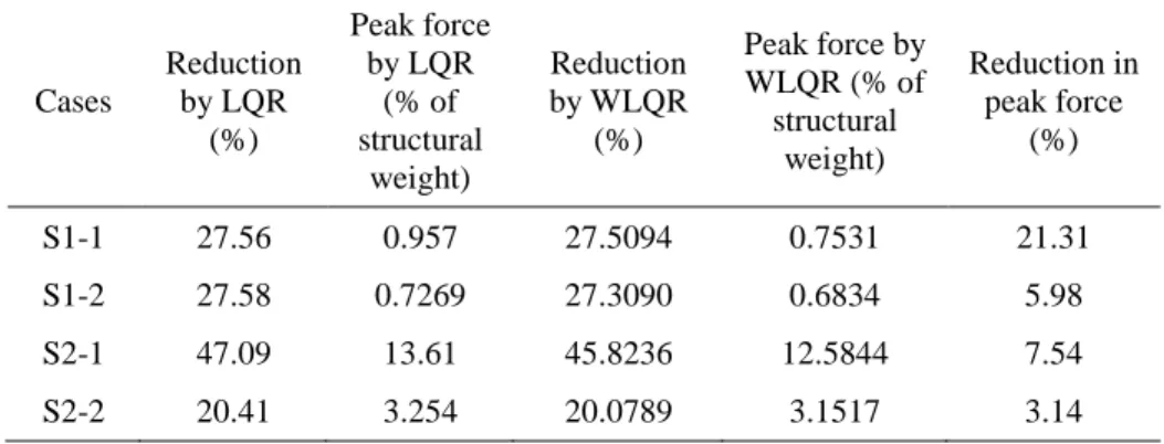
𝑆2 − 1 and 𝑆2 − 2 respectively. The reduction in structural displacement response obtained by the WLQR algorithm and corresponding maximum required control force for the different cases are presented in Table 6 and compared with the results obtained by the LQR algorithm. It is observed that a reduction of as high as 21.31 % in the peak control force could be achieved by the WLQR controller, without compromising the response reduction achieved by the ACLCD. It is also observed that for lower values of length ratio, 𝛼, (cases 𝑆1 − 1 and 𝑆2 − 1) the reduction in force is higher in case of both example structures.

Representative time history results for structural displacement, control force, liquid displacement and whole damper displacement for the example flexible (𝑆1 − 2) and stiff (𝑆2 − 2) structures are shown in Figs. 15 and 16 respectively.

Figure 15 Figure 16

(18)

Now, it has been seen from Fig. 11d that for the LQR controller, the response reduction increases for case 𝑆2 − 2 for higher values of 𝜉. It is thus interesting to examine the performance of the WLQR controller under the same conditions. For this, the control parameters for 𝜉 equal to 51 are chosen, which are 𝑞_𝑜𝑝𝑡(𝑆2)

𝑎 = 4 × 10 11_,_𝑅

𝑎5 = 𝑅𝑎4 = 0.0006 as obtained from the LQR

algorithm. Now by several trials the WLQR controller is designed with the optimum 𝑅_𝑎 value for the low energy frequency bands obtained as 0.008. The peak response reduction and corresponding maximum required control force as obtained by the WLQR controller are 43.51 % and 8.824 % of structural weight respectively. In comparision, the response reduction obtained by the LQR controller is 44.33 % with maximum control force requirement of 10.31 % of structural weight. Thus, a reduction in peak control force of 14.42 % is achieved by the WLQR controller over the LQR controller, which is higher than that obtained with a lower 𝜉 value (see Tables 1 and 2 for case 𝑆2 − 2).

Performance of designed WLQR controller against excitation variability

As in case of the LQR controller, the performance of the designed WLQR controller is examined for base excitations other than the earthquake data used for the design. Previously mentioned Parkfield and Taft earthquake data are used for this study. The test cases mentioned in Table 4 are also considered here. The frequency dependent gains [𝐺]𝑎𝑙 and [𝐺]𝑎𝑗 are calculated for the El

Centro earthquake data using the corresponding values of 𝑅𝑎. With these frequency dependent gains, the equivalent time varying gain, [𝐺𝑒(𝑡)], and the control force are evaluated for Parkfield and Taft input data. The response reductions achieved without violating the constraints and the corresponding required peak control forces are presented in Table 7. The performances of the WLQR and LQR controllers are also compared from Table 4. It is observed that the WLQR controller performs well under excitation variability and here too the WLQR controller can achieve a comparable response reduction as obtained by LQR controller with lower requirement of peak control force.

Figs. 17 and 18 present the representative time history results for structural displacement and control force generated by the WLQR controller for flexible (𝑆1 − 2) and stiff (𝑆2 − 2) structures respectively.

(19)

Figure 18

A maximum of 21.23 % reduction in peak control force is achieved by the WLQR algorithm over the LQR algorithm, which again demonstrates the efficiency of the WLQR algorithm. Conclusions

(20)

founded on some filtering mechanisms (due to the filtering property of the wavelet transform) and hence the high frequency noises are automatically eliminated.

Acknowledgement :

This study was supported by

 Department of Science and Technology (DST), Govt. of India (Sanction Order No: SR/S3/MERC-0017/2012 dated 18th May, 2012).

 Science Foundation Ireland (SFI) under the International Strategic Cooperation Award (Grant Number SFI/12/ISCA/2493)

References:

[1] Saoka Y, Sakai F, Takaeda S, Tamaki T. On the suppression of vibrations by tuned liquid

column dampers. Proceedings of Annual Meeting of JSCE, Tokyo 1988.

[2] Sakai F, Takaeda S, Tamaki T. Tuned liquid column damper – new type device for

suppression of building vibrations. Proceedings of International Conference on Highrise Buildings, Nanjing, China 1989; 926-931.

[3] Xu YL, Samali B, Kwok KCS. Control of along – wind response of the structures by

mass and liquid dampers. Journal of Engineering Mechanics, ASCE 1992; 118(1): 20-39.

[4] Balendra T, Wang CM, Cheong HF. Effectiveness of tuned liquid column dampers for

vibration control of towers. Engineering Structures 1995; 17(9): 668-675.

[5] Wu JC, Shih MH, Lin YY, Shen YC. Design guidelines for tuned liquid column damper

for structures responding to wind. Engineering Structures 2005; 27(13): 1893-1905.

[6] Zhang Z, Basu B, Nielsen SRK. Tuned liquid column dampers for mitigation of edgewise

vibrations in rotating wind turbine blades. Structural Control and Health Monitoring 2015; 22(3): 500-517.

[7] Zhang Z, Staino A, Basu B, Nielsen SRK. Performance evaluation of full-scale tuned

liquid dampers (TLDs) for vibration control of large wind turbines using real-time hybrid testing, Engineering Structures 2016; 126: 417-431.

[8] Sun K. Earthquake responses of buildings with liquid column dampers. Proceedings of

5th U. S. National Conference on Earthquake Engineering, Chicago 1994; II: 411-420.

[9] Won AYJ, Pires JA, Haroun MA. Stochastic seismic evaluation of tuned liquid column

(21)

[10] Sadek F, Mohraz B, Lew HS. Single and multiple tuned liquid column dampers for

seismic applications. Earthquake Engineering and Structural Dynamics 1998; 27: 439-463.

[11] Yalla SK, Kareem A. Optimum absorber parameters for tuned liquid column dampers.

Journal of Structural Engineering 2000; 126(8): 906-915.

[12] Ghosh A, Basu B. Alternative approach to optimal tuning parameter of liquid column

damper for seismic applications. Journal of Structural Engineering, ASCE 2007; 133(12): 1848-1852.

[13] Ghosh A, Basu B. Seismic vibration control of nonlinear structures using the liquid

column damper. Journal of Structural Engineering, ASCE 2008; 134(1): 146-153.

[14] Sakai F, Takaeda S, Tamaki T. Tuned liquid damper (TLCD) for cable stayed bridges.

Proceedings of Specialty Conf. Invitation in Cable-Stayed Bridges, Fukuoka, Japan 1991; 197-205.

[15] Teramura A, Yoshida O. Development of vibration control system using U-shaped water

tank. Proceedings of the Eleventh World Conference on Earthquake Engineering, Pergamon 1996; Paper No. 1343.

[16] Kareem A. The next generation of tuned liquid dampers. Proceedings of First World

Conference on Structural Control, Los Angeles, California, USA 1994; FP5 19-FP5 28.

[17] De Corte W, Delesie C, Bogaert PV. Sealed tuned liquid column dampers: a cost

effective solution for vibration damping of large arch hangers. Proceedings of 5th International Conference on Arch Bridges, Madeira, Portugal 2007; 409-416.

[18] Reiterer M, Ziegler F. Bi-axial seismic activation of civil engineering structures equipped

with tuned liquid column dampers. JSEE: Spring 2005; 7(1): 45-60.

[19] Ghosh A, Basu B. Seismic vibration control of short period structures using the liquid

column damper. Engineering Structures 2004; 26: 1905-1913.

[20] Ghosh A, Basu B. Compliant liquid column dampers for control of seismically excited

short period structures. Proceedings of 1st European Conference on Earthquake Engineering and Seismology, Geneva, Switzerland 2006.

[21] Gur S, Mishra SK, Bhowmick S, Chakraborty S. Compliant liquid column damper

(22)

[22] Bhattacharyya S, Ghosh AD, Basu B. Experimental investigations into CLCD with

identification of tuning and damping effects. Journal of Structural Engineering 2017; 143(9).

[23] Balendra T, Wang CM, Yan N. Control of wind-excited towers by active tuned liquid

column damper. Engineering Structures 2001; 23(9): 1054-1067.

[24] Chen YH, Ko CH. Active tuned liquid column damper with propellers. Earthquake

Engineering and Structural Dynamics 2003; 32:1627–1638. (DOI: 10.1002/eqe.295)

[25] Hochrainer MJ, Ziegler F. Control of tall building vibrations by sealed tuned liquid

column dampers. Structural Control and Health Monitoring 2006; 13: 980-1002.

[26] Haroun MA, Pires JA, Won AY. Suppression of environmentally‐ induced vibrations in

tall buildings by hybrid liquid column dampers. The Structural Design of Tall and Special Buildings 1996; 5(1): 45-54.

[27] Kim H, Adeli H. Hybrid control of smart structures using a novel wavelet-based

algorithm. Computer –aided Civil and Infrastructure Engineering 2005; 1 (20): 7-22.

[28] Yalla SK, Kareem A, Kantor JC. Semi-active tuned liquid column dampers for vibration

control of structures. Engineering Structures 2001; 23: 1469–1479.

[29] Yalla SK, Kareem A. Semi-active tuned liquid column dampers: experimental study.

Journal of Structural Engineering 2003; 129(7): 960-971.

[30] Li HN, Huo LS. Seismic control of eccentric structures using TLCD semi-active neural

networks. Proceedings of IEEE Conference on Control Applications, Istanbul, Turkey 2003; 1: 336-340.

[31] Li HN, Jin Q, Song G, Wang GX. Fuzzy neural network based TLCD semi-active control

methodology for irregular buildings. Proceedings of IEEE International Symposium on intelligent Control, Houston Texas 2003.

[32] Bigdeli Y, Kim D. Response control of irregular structures using structure-TLCD coupled

system under seismic excitations. KSCE Journal of Civil Engineering 2015; 19(3): 672-681.

[33] Sonmez E, Nagarajaiah S, Sun C, Basu B. A study on semi-active Tuned Liquid Column

(23)

[34] Ni YQ, Ying ZG, Wang JY, Ko JM, Spencer Jr. BF. Stochastic optimal control of

wind-excited tall buildings using semi-active MR-TLCDs. Probabilistic Engineering Mechanics 2004; 19: 269–277.

[35] Wang DH, Liao WH. Semiactive controllers for magnetorheological fluid dampers.

Journal of Intelligent Material Systems and Structures 2005; 16(11-12): 983-993.

[36] Colwell S, Basu B. Experimental and theoretical investigations of equivalent viscous

damping of structures with TLCD for different fluids. Journal of Structural Engineering 2008; 134(1): 154-163.

[37] Basu B, Bursi OS, Casciati F, Casciati S, Del Grosso AE, Domaneschi M, Faravelli L,

Holnicki-Szulc J, Irschik H, Krommer M, Lepidi M, Martelli A, Ozturk B, Pozo F, Pujol G, Rakicevic Z, Rodellar J. A European association for the control of structures joint perspective. Recent studies in civil structural control across Europe. Structural Control and Health Monitoring 2014; 21: 1414-1436.

[38] Basu B, Nagarajaiah S. A multi-scale wavelet LQR controller for linear time varying

systems. Journal of Engineering Mechanics, ASCE 2010; 136(9): 1142 – 1150.

[39] Kyprianou A, Staszewski WJ. On the cross wavelet analysis of duffing oscillator. Journal

of Sound and Vibration 1999; 228(1): 199-210.

[40] Staszewski WJ. Identification of damping in MDOF systems using time-scale

decomposition. Journal of Sound and Vibration 1997; 203(2): 283-305.

[41] Staszewski WJ, Robertson AN. Time-frequency and time-scale analyses for structural

health monitoring. Philosophical Transactions of the Royal Society A 2007; 365(1851).

[42] Staszewski WJ, Wallace DM. Wavelet-based frequency response function for

time-variant systems – an exploratory study. Mechanical Systems and Signal Processing 2014; 47(1-2): 35-49.

[43] Chakraborty A, Basu B. Analysis of frequency nonstationarity via continuous wavelet

transform in the response of primary-secondary systems. Journal of Structural Engineering 2010; 136(12): 1608-1612.

[44] Basu B, Nagarajaiah S. A wavelet-based time-varying adaptive LQR algorithm for

(24)

Table 1. Optimal damper parameters of passive CLCD and corresponding response reductions, liquid and whole damper displacements

Case designation 𝑆1 − 1 𝑆1 − 2 𝑆2 − 1 𝑆2 − 2

𝛼 0.4 0.7 0.4 0.7

𝜈𝑜𝑝𝑡 0.7 0.7 0.8 0.7

𝜉𝑜𝑝𝑡 3 43 1 2

Peak reduction in structural

displacement (%) 19.60 19.57 15.77 11.44

Peak liquid displacement

(m) 0.71 0.28 0.18 0.27

Peak whole damper

displacement (m) 0.96 0.78 0.37 0.34

Table 2. 𝑞_𝑜𝑝𝑡(𝑆𝑖) for different values of 𝑅, and corresponding peak reductions in structural displacement and peak control force, for designed ACLCD by LQR algorithm for cases 𝑆𝑖 − 𝑘 (𝑖 = 1, 2; 𝑘 = 1, 2)

Cases Serial No. 𝑅 𝑞_𝑜𝑝𝑡(𝑆𝑖)

Peak reduction in structural displacement (%)

Peak control force (% of structural weight)

𝑆1 − 1

1 0.0004 4 × 1010 27.56 0.994

2 0.0005 4 × 1010 27.56 0.957

3 0.001 4 × 1010 27.55 0.883

4 0.01 4 × 1010 27.43 0.717

5 0.1 4 × 1010 26.49 0.616

6 1 5 × 1010 24.85 0.475

7 10 1 × 1011 23.36 0.315

8 100 6 × 1011 23.64 0.273

𝑆1 − 2

1 0.0006 4 × 1010 27.70 0.7525

2 0.001 4 × 1010 27.69 0.7490

3 0.01 4 × 1010 27.58 0.7269

4 0.1 4 × 1010 26.50 0.6339

5 1 4 × 1010 22.91 0.9370

6 10 9 × 1010 22.17 0.2904

7 100 4 × 1011 21.71 0.2027

𝑆2 − 1

1 0.0005 6 × 1011 47.09 13.610

2 0.001 6 × 1011 46.40 12.780

3 0.01 8 × 1011 44.02 10.510

4 0.1 2 × 1012 41.26 8.771

(25)

6 10 1 × 1014 39.12 7.940

𝑆2 − 2

1 0.0006 5 × 1010 20.41 3.254

2 0.001 5 × 1010 20.27 3.229

3 0.01 7 × 1010 22.11 2.944

4 0.1 8 × 1010 18.92 2.313

5 1 1.3 × 1011 14.98 1.342

6 10 5 × 1011 14.25 0.834

7 100 4 × 1012 14.44 0.751

Table 3. Response reductions obtained by ACLCD and corresponding maximum required force compared with that obtained by passive CLCD for 𝑆1 and 𝑆2

Case designation 𝑆1 − 1 𝑆1 − 2 𝑆2 − 1 𝑆2 − 2

Maximum peak reduction in structural displacement obtained

by ACLCD (%)

27.56 27.70 47.09 22.11

Maximum peak reduction in structural displacement obtained

by passive CLCD (%)

19.60 19.57 15.77 11.44

Table 4. Peak reductions in structural displacement and corresponding maximum control force obtained for designed ACLCD by LQR algorithm against excitation variability

Earthquake data Case

LQR algorithm Peak reduction in

structural displacement (%)

Peak control force (% of structural

weight)

El Centro 𝑆1 − 2 27.70 0.753

𝑆2 − 2 20.41 3.254

Parkfield 𝑆1 − 2 33.74 0.607

𝑆2 − 2 28.84 2.369

Taft 𝑆1 − 2 30.35 0.479

𝑆2 − 2 28.37 1.424

Uttarkashi 𝑆1 − 2 12.42 1.132

𝑆2 − 2 26.38 2.064

Chamoli 𝑆1 − 2 44.10 0.639

𝑆2 − 2 13.02 2.339

Mammoth Lakes 𝑆1 − 2 34.40 0.327

(26)

Table 5. Central frequencies of the frequency bands of decomposed response signal at each level

Frequency band

number 7 6 5 4 3 2 1

Central frequency

(rad/s) 1.753 3.506 7.013 14.025 28.050 56.100 112.200

Table 6. Response reductions obtained by WLQR algorithm and corresponding maximum required force compared with that obtained by LQR algorithm for 𝑆1 and 𝑆2

Cases Reduction by LQR (%) Peak force by LQR (% of structural weight) Reduction by WLQR (%)

Peak force by WLQR (% of

structural weight)

Reduction in peak force

(%)

S1-1 27.56 0.957 27.5094 0.7531 21.31

S1-2 27.58 0.7269 27.3090 0.6834 5.98

S2-1 47.09 13.61 45.8236 12.5844 7.54

S2-2 20.41 3.254 20.0789 3.1517 3.14

Table 7. Peak reductions in structural displacement and corresponding maximum control force obtained for designed ACLCD by WLQR algorithm against excitation variability

Earthquake

data Case

WLQR algorithm Reduction in peak force (%) Peak reduction (%) Peak control force (% of

structural weight)

El Centro 𝑆1 − 2

27.3 0.683 9.18

𝑆2 − 2 20.1 3.152 3.13

Parkfield 𝑆1 − 2

33.4 0.478 21.23

𝑆2 − 2 28.6 2.192 7.46

Taft 𝑆1 − 2 30.0 0.407 14.98

𝑆2 − 2 28.0 1.406 1.31