Automatic Detection and Tracking of CMEs II:
Multiscale Filtering of Coronagraph Images
Jason P. Byrne
1, Huw Morgan
1,2, Shadia R. Habbal
1and Peter T. Gallagher
3 1Institute for Astronomy, University of Hawai’i, 2680 Woodlawn Drive, Honolulu, HI 96822, USA.2Institute of Mathematics and Physics, Aberystwyth University, Ceredigion, Wales, SY23 3BZ. 3Astrophysics Research Group, School of Physics, Trinity College Dublin, Dublin 2, Ireland.
ApJ, 752, 145. doi:10.1088/0004-637X/752/2/145
ABSTRACT
Studying CMEs in coronagraph data can be challenging due to their diffuse structure and transient nature, and user-specific biases may be introduced through visual inspection of the images. The large amount of data available from the SOHO, STEREO, and future coronagraph missions, also makes manual cataloguing of CMEs tedious, and so a robust method of detection and analysis is required. This has led to the development of automated CME detection and cata-loguing packages such as CACTus, SEEDS and ARTEMIS. Here we present the development of a new CORIMP (coronal image processing) CME detection and tracking technique that overcomes many of the drawbacks of current catalogues. It works by first employing the dynamic CME separation technique outlined in a companion paper, and then characterising CME structure via a multiscale edge-detection algorithm. The detections are chained through time to determine the CME kinematics and morphological changes as it propagates across the plane-of-sky. The effectiveness of the method is demonstrated by its application to a selection of SOHO/LASCO and STEREO/SECCHI images, as well as to synthetic coronagraph images created from a model corona with a variety of CMEs. The algorithms described in this article are being applied to the whole LASCO and SECCHI datasets, and a catalogue of results will soon be available to the public.
Subject headings: Sun: activity; Sun: corona; Sun: coronal mass ejections (CMEs); Techniques: image processing
1. Introduction
Coronal mass ejections (CMEs) are large-scale eruptions of plasma and magnetic field from the Sun into interplanetary space, and have been studied extensively since they were first dis-covered four decades ago (Tousey & Koomen 1972). They propagate with velocities ranging from ∼20 km s−1 to over 2000 km s−1 (Yashiro
et al. 2004; Gopalswamy et al. 2001), and with masses of 1014– 1017 g (Jackson 1985; Hudson
et al. 1996; Gopalswamy & Kundu 1992), and are a significant driver of space weather in the near-Earth environment and throughout the
he-liosphere (Schrijver & Siscoe 2010; Schwenn et al. 2005). Traveling through space with average mag-netic field strengths of 13 nT (Lepping et al. 2003) and energies of∼1025J (Emslie et al. 2004), they can cause geomagnetic storms upon impacting Earth’s magnetosphere, possibly damaging satel-lites, inducing ground currents, and increasing the radiation risk for astronauts (Lockwood & Hap-good 2007). Thus, models of CMEs and the forces acting on them during their eruption and propa-gation through the corona remain an active area of research (see reviews by Chen 2011; Webb & Howard 2012).
The Large Angle Spectrometric Coronagraph
suite (LASCO; Brueckner et al. 1995) onboard the Solar and Heliospheric Observatory (SOHO; Domingo et al. 1995) has observed thousands of CMEs from 1995 to present; and since 2006 the Sun-Earth Connection Coronal and Heliospheric Imaging suite (SECCHI; Howard et al. 2008) on-board the Solar Terrestrial Relations Observatory (STEREO; Kaiser et al. 2008) has provided twin-viewpoint observations of the Sun and CMEs from off the Sun-Earth line. Defined as an outwardly moving, bright, white-light feature, CMEs appear in a variety of geometrical shapes and sizes, typi-cally exhibiting a three-part structure of a bright leading front, dark cavity, and bright core (Illing & Hundhausen 1985). Their geometry is attributed to the underlying magnetic field, generally be-lieved to have a flux-rope configuration. The erup-tion of the CME is triggered by a loss of sta-bility and its subsequent outward motion is gov-erned by the interplay of magnetic and gas pres-sure forces in the low plasma-β environment of the solar corona. CMEs are commonly linked to filament/prominence eruptions and solar flares (Moon et al. 2002; Zhang & Wang 2002), or la-belled ‘stealth CMEs’ if they cannot be associ-ated with any on-disk activity (Robbrecht et al. 2009), but knowledge about their specific driver mechanisms remains elusive. Several theoretical models have been developed in order to describe the forces responsible for the observed characteris-tics of CME initiation and propagation. The most favoured models explain CMEs in the context of tether straining and release, whereby the outward magnetic pressure increases due to flux injection or field shearing, and overcomes the magnetic ten-sion of the overlying field (Klimchuk 2001). Dif-ferent approaches to such models provide difDif-ferent force-balance interpretations, that lead to a vari-ety of predictions on the kinematic and morpho-logical evolution of CMEs (e.g. Priest & Forbes 2002; Chen & Krall 2003; Kliem & T¨or¨ok 2006; Lynch et al. 2008). To this end, there is a moti-vation to resolve the obsermoti-vations of CMEs with robust, high-accuracy methods, in order to deter-mine their kinematics and morphology with the greatest possible precision.
From the large number of CMEs observed to date, many exhibit a general multiphased kine-matic evolution. This often consists of an initi-ation phase, an acceleriniti-ation phase, and a
propa-gation phase which can show positive or negative residual acceleration as the CME speed equalizes to that of the local solar wind (Zhang & Dere 2006; Maloney et al. 2009). Statistical analyses can pro-vide a general indication of CME properties (e.g. Gopalswamy et al. 2000; dal Lago et al. 2003; Schwenn et al. 2005), but it remains true that indi-vidual CMEs must be studied with rigour in order to satisfactorily derive the kinematics and mor-phology to be compared with theoretical models. The CME catalogue hosted at the Coordinated Data Analysis Workshop (CDAW1) Data Center
grew out of a necessity to record a simple but ef-fective description and analysis of each event ob-served by LASCO (Gopalswamy et al. 2009), but its manual operation is both tedious and subject to user biases. Ideally an automated method of CME detection should be applied to the whole LASCO and SECCHI datasets in order to glean the most information possible from the available statistics. A number of catalogues have therefore been de-veloped in an effort to do this, namely the Com-puter Aided CME Tracking catalogue (CACTus2; Robbrecht & Berghmans 2004), the Solar Eruptive Event Detection System (SEEDS3; Olmedo et al. 2008) and the Automatic Recognition of Tran-sient Events and Marseille Inventory from Synop-tic maps (ARTEMIS4; Boursier et al. 2009).
How-ever, these automated catalogues have their limi-tations. For example CACTus imposes a zero ac-celeration, while SEEDS and ARTEMIS employ only LASCO/C2 data. The motivation thus ex-ists to develop a new automated CME detection catalogue that overcomes such drawbacks, and in-deed methods of multiscale analysis have shown excellent promise for achieving this (Byrne et al. 2009).
In this paper we discuss a new coronal im-age processing (CORIMP) technique for detect-ing and trackdetect-ing CMEs. We outline our appli-cation of an automated multiscale filtering tech-nique, to remove small scale noise/features and enhance the larger scale CME in single corona-graph frames. This allows the CME structure to be detected with increased accuracy for deriving
1http://cdaw.gsfc.nasa.gov/CME list 2http://sidc.oma.be/cactus/
the event kinematics and morphology. A compan-ion paper (Morgan et al. 2012, hereafter referred to as Paper I) outlines the steps used in prepro-cessing the coronagraph data with a normalizing radial graded filter (NRGF; Morgan et al. 2006) and deconvolution technique for removing the qui-escent background features, leading to a very clean input for the automatic CME detection algorithm. These image processing steps are based on ideas first developed by Morgan & Habbal (2010), where a more rudimentary approach was taken to isolate the dynamic component of coronagraph images. The new methods of Paper I, in conjunction with those outlined here, have led to a significant im-provement in our ability to automatically detect and track CMEs in coronagraph data, such that a wealth of information on their structure and evo-lution may be obtained.
In Section 2 we outline the multiscale filter-ing techniques employed, and our method of au-tomatically detecting and tracking CMEs in coro-nagraph images. In Section 3 the effectiveness of the CORIMP algorithms is demonstrated through their application to sample cases of LASCO and SECCHI data, and to a model corona with CMEs of known morphology. In Section 4 we discuss the results and conclusions from the techniques.
2. Automated CME Detection And
Track-ing
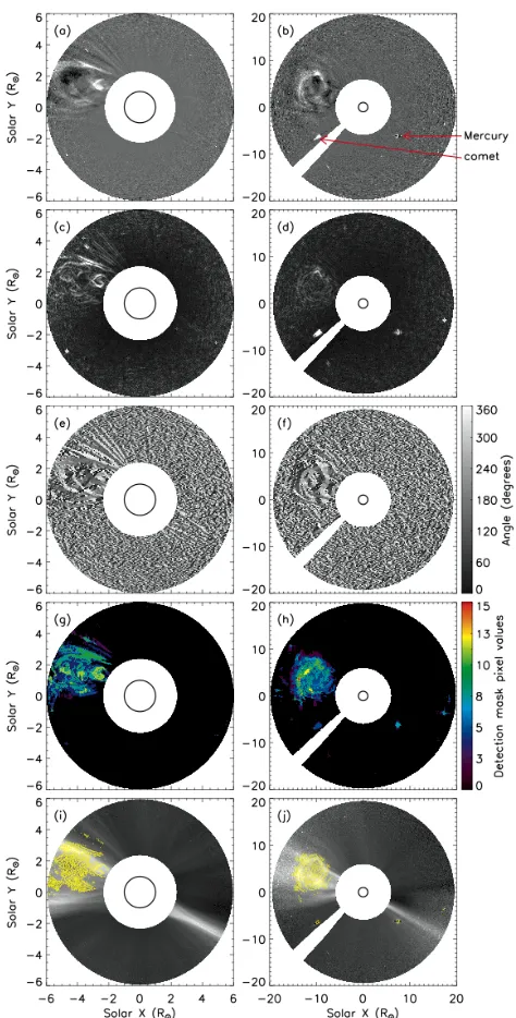
Figures 1a and 1b show a LASCO/C2 and C3 image of a CME on 2010 March 12 at times 05:06 and 11:42 UT respectively, having been pro-cessed as per the techniques of Paper I (namely the NRGF and quiescent background separation). The CME is somewhat ill-defined in the C2 im-age, consisting of a complex loop structure sur-rounded by streamer material. In the C3 image the CME has a clearer three-part structure con-sisting of a bright front, dark cavity, and trailing core. A comet and the planet Mercury are also visible in the C3 field-of-view.
In order to avoid introducing unwanted edge ef-fects with the automated detection technique, i.e., to prevent the occulter/field-of-view edges from dominating the detection, the image data is nu-merically reflected inwards and outwards of the occulted field-of-view in the image. This acts to smooth out the sudden change of intensity at the
limits of the field-of-view, that would otherwise be detected as significant edges along the boundaries of the image data. The strength of the occulter edges would also suppress the true structure lying close to the occulter edge in the image, somewhat limiting the image area eligible for CME detection by a factor dependent on each particular scale of the multiscale decomposition.
2.1. Multiscale Filtering
A multiscale filter is applied as outlined in Young & Gallagher (2008) and shown by Byrne et al. (2009, 2010); Gallagher et al. (2011); P´ erez-Su´arez et al. (2011) to be effective for studying CMEs in coronagraph data. The fundamental idea behind multiscale analysis is to highlight details apparent on different scales within the data. Noise can be effectively suppressed, since it tends to oc-cur only on the smallest scales. Wavelets, as a multiscale tool, have benefits over previous meth-ods, such as Fourier transforms, because they are localised in space and are easily dilated and trans-lated in order to operate on multiple scales. The fundamental equation describing the filter is given by:
ψa,b(t) =
1
√
bψ( t−a
b ) (1)
where aandb represent the shifting (translation) and scaling (dilation) of the mother wavelet ψ
which can take several forms depending on the required use. Here, a method of multiscale de-composition in 2D is employed, through the use of low and high pass filters; using a discrete ap-proximation of a Gaussian, θ, and its derivative,
ψ, respectively. Since θ(x, y) is separable, i.e.,
θ(x, y) = θ(x)θ(y), we can write the wavelets as the first derivative of the smoothing function:
ψxs(x, y) = s−2∂θ(s−1x)
∂x θ(s
−1y) (2)
ψys(x, y) = s−2θ(s−1x)∂θ(s∂y−1y) (3)
wheresis the dyadic scale factor such thats= 2j forj = 1,2,3, ..., J ∈ N. Successive convolutions
of an image with the filters produce the scales of decomposition, with the high-pass filtering provid-ing the wavelet transform of imageI(x, y) in each direction:
WxsI ≡ Ws
xI(x, y) = ψxs(x, y)∗I(x, y) (4)
WysI ≡ Ws
Akin to a Canny edge detector, these horizontal and vertical wavelet coefficients are combined to form the gradient space, Γs(x, y), for each scale:
Γs(x, y) =
WxsI, WysI
(6)
The gradient information has an angular compo-nentαand a magnitude (edge strength)M:
αs(x, y) = tan−1 WysI / WxsI
(7)
Ms(x, y) = q(Ws
xI)2+ (WysI)2 (8)
Figures 1c and 1d show the magnitude infor-mation (with intensity showing the relative edge strengths), and Figures 1e and 1f the angular in-formation, for a particular scale (s = 24) of the
multiscale decomposition applied to the CME im-ages of Figures 1a and 1b. As the figures show, the inherent structure of the CME is highlighted very effectively, along with the comet, the planet Mer-cury, any residual streamer material, and some of the brighter stars. Figures 1e and 1f show the an-gular component αof the gradient, that specifies a direction normal to the intensity regions of the magnitude information M. Thus a pixel-chaining algorithm may be employed to trace out all of the multiscale edges in the image, using the orthogo-nal direction of the angular information as criteria for chaining pixels along the local maxima of the magnitude information.
2.2. CME Detection Mask
The scales upon which the multiscale filter-ing best resolves the CME have dyadic scale fac-tors of s = 22, 23,24,25. The discarded finer
scales mostly detail the noise, and the coarser scales overly smooth the CME signal. At each of these four scales, the corresponding magnitude
M is thresholded at 1.5σ (σ is the standard de-viation) above the mean intensity level, resulting from inspection of the method applied to a sam-ple of ten different CMEs of varying speeds, widths and noise levels. This results in regions-of-interest (ROIs) on each image that may be tested as CMEs since they meet the criterion that they are bright features, consequently having stronger edges. To make the 1.5σthreshold somewhat softer, the ini-tial ROIs are removed and the threshold reapplied at 1.5σof the remaining image data to obtain new ROIs. The difference between the new and
orig-inal ROIs is quantified by subtracting the num-ber of pixels in each, and the intensity threshold reapplied if the subsequent ROI pixel difference is greater than the preceding difference. If the quan-tified difference decreases, signaling that nothing more can be gained by continuing to soften the threshold on the magnitude image, the threshold is fixed and used to determine the final ROIs. The angular information is then determined for each of these ROIs, since a curvilinear feature will have a wider distribution of angles than a radial fea-ture or a point source in the decomposition. The angular distributions of the individual ROIs are rescaled from ranges 0 – 360◦ to 0 – 180◦ due to their axial symmetry, and the distribution is nor-malized to unity. The median value of the dis-tribution across each ROI is then thresholded as a measure for scoring the validity of the detection in order to build up a detection mask of the image:
1. If the median angular value is>20% of the distribution peak then the region is deemed a CME and assigned a score of 3 (the pixels in that ROI are given the value 3).
2. If it is between 10 – 20% the score is 2 (po-tential CME structure).
3. If it is between 5 – 10% the score is 1 (weak CME structure or part thereof).
Figures 1g and 1h show the resulting CME de-tection mask generated from the additive accu-mulation of the scores at each scale used for the LASCO/C2 and C3 images. Immediately it is pos-sible to remove the areas of the mask that do not additively achieve a strong enough detection. So, again by inspection across the test sample of ten events, the masks are thresholded at a level >3 since only the regions that accumulate a sufficient score to be classified as a CME detection are in-cluded.
somewhat reduced by removing the lowest scoring regions of the detection mask as discussed above, but is further corrected for by eroding the detec-tion mask by a factor of 8 pixels. This factor is half the filter width at scale s= 24 chosen based
on the fact that if the lowest scale (s= 25) ROIs in the detection mask have been removed, then the CME edge being detected will likely be situated half the next filter width (s = 24) inside of the detection mask boundary. Figures 1i and 1j show the resultant CME structure detections overlaid on the original images. While there is still an el-ement of noise in the detections, clear structure along the twisted magnetic field topology of the erupting CME plasma is defined - and automati-cally so.
2.3. Determining The Physical
Character-istics Of Detected CMEs
The outermost points along the strongest de-tected edges of the CME structure provide the CME height from Sun-center in each image. To determine these so-called strongest edges, the magnitude information deduced from each of the four scales in use here, are multiplied together to enhance the strongest features, and the result-ing strengths are assigned to the relative pixels of the edge detections. One median absolute devi-ation above the median strength of the edges is used as a threshold for determining the strongest edges within the detected CME structure (as op-posed to one standard deviation above the mean, which is too easily affected by bright stars, plan-ets, noisy features etc.). The outermost points of these strongest edges, measured along radial lines drawn at 1◦position angle intervals, are recorded as the span of CME heights in each frame.
As the detections are performed through time, the information from them may be collated into a three-dimensional stack of ‘Time’ versus ‘Posi-tion Angle’ versus ‘Height’. A CME detected at a particular span of position angles through a se-quence of frames will appear as a block of variable height in the detection stack, an example of which is shown in Figure 2 (following some further pro-cessing via a cleaning algorithm outlined below). The detection stack for the LASCO data contain-ing the CME shown in Figure 1 is illustrated in the top part of Figure 2; while the detection stack for the interval from 2010 February 27 to March 5
is illustrated in the bottom part, as an example of several typical detections during an active period when Jupiter was also in the field-of-view. The angular span of the detections is indicative of the angular width of the CME. Trailing material con-tained within the internal structure of the CME will also be apparent on the detection stack as the CME front moves out of the field-of-view. Any residual streamer flows that are detected will also appear in the detection stack, though they should only span small angular widths. Because the 2010 March 12 CME has a lot of internal and trailing material, the persistent C2 material detections un-derly the increasing C3 height detections, as indi-cated by the somewhat constant purple shade em-bedded in the CME-specific region of the detection stack in the top of Figure 2. This example demon-strates how the codes fare with typical issues faced in CME image data, while also demonstrating its success alongside the additional comet and planet detections. Other CMEs will have cleaner profiles than this one, as some of the detections in the bot-tom plot show. The comet detection height profile shows a decreasing color intensity in time due to its decreasing height as it falls toward the Sun. The planets Mercury and Jupiter show a change in position angle, along with a slight change in height, as they traverse the fields-of-view. Some random detections due either to small-scale flows, noisy features or artifacts in the images are also apparent in the detection stack, mostly concen-trated along the streamer belts centered at posi-tion angles∼90◦ and∼270◦.
For the purposes of cataloguing CMEs, a clean-ing algorithm was developed and applied to the tection stack to remove much of the noise. The de-tection stack regions corresponding to CMEs may be automatically isolated by the following criteria:
1. Detections that lie within two time steps of each other are grouped.
3. Detections that have not been grouped with at least two other detections are discarded.
The resulting detection stack provides a cleaner output for determining the CME kinematics and morphology. The height information at each po-sition angle of the isolated detection groups may be recorded and used to build a height-time pro-file across the angular span of the detection. Since there exists the possibility that persistent C2 de-tections can underly the C3 dede-tections of a CME, conditions are imposed on the code to retrieve the height-time profile in a manner such that once the CME height along each position angle moves beyond the C2 field-of-view, only its subsequent heights within the C3 field-of-view are recorded. Examples of CME height-time profiles recorded in this way are shown in Section 3.1. Changes in the angular width of a CME detection may also be recorded as an indicator of its expan-sion. Thus a final output of information on each CME detection can include CME height, obser-vation time, position angle, trajectory, and angu-lar width. Due to the various methods available for determining kinematics from height-time mea-surements (e.g., standard numerical differentia-tion techniques, spline fitting techniques, inversion techniques; see Temmer et al. 2010 for example), an investigation of the best approach for catalogu-ing the specific kinematics of CMEs is postponed to future work. Furthermore, the morphological information that can be attained with these meth-ods, arising from the pixel-chained edge detections and overall enhancement of structure within the CME, will facilitate future detailed inspections of the observed ejection material.
3. Testing On Real And Synthetic Data
In order to test how well the CME structure is resolved by these automated methods, the algo-rithm is applied to a selection of real data from the LASCO and SECCHI coronagraphs, and to synthetic data comprising a model corona through which CMEs of various appearance are propa-gated. We consider first the real data, which is processed according to the methods outlined in Paper I, namely the NRGF and dynamic separa-tion techniques.
3.1. LASCO And SECCHI CME Data
The automated CME detection technique is ap-plied to LASCO/C2 and C3, and SECCHI/COR2-A and B coronagraph images. For these algo-rithms, the C2 images have a workable field-of-view of 2.35 – 5.95 R, while C3 is limited to 5.95 –
19.5 R (of a potential∼30 R) since the
signal-to-noise ratio is too low in the outermost portion of its field-of-view to be used for automatically iden-tifying CMEs via these methods. The SECCHI coronagraphs have a workable field-of-view of 3 – 11 R for COR2-A, and 4.5 – 11 R for COR2-B
(of a potential ∼3 – 15 R), again limited by the
low signal-to-noise ratio. COR1 proved unfeasi-ble for analysis since the non-radial profile of the corona at heights <3 R does not fare well with
the NRGF, and the images have too low a signal-to-noise ratio for the automated techniques to op-erate satisfactorily.
Figure 3 (and its online animation) shows a sample output of the automated detections on LASCO observations of CMEs dated 2000 January 2, 2000 April 18, 2000 April 23, and 2011 January 13. The four CMEs are shown for instances of their detection in C2 and C3, along with the re-sulting height-time profiles corresponding to the tracks of the strongest outermost front (red points on CMEs) of the overall detected structure (yel-low points on CMEs). Each of these profiles has an associated colorbar that indicates the relevant position angle along which the heights are mea-sured. The 2000 January 2 CME exhibits a multi-loop structure, and its height-time profile indicates a relatively constant velocity as it catches up to slower moving material along its southern path. The 2000 April 18 CME has a typical 3-part struc-ture, and its height-time profile shows early accel-eration, and some trailing ejecta along its western flank. The 2000 April 23 CME is a highly im-pulsive partial halo, and its height-time profile is accordingly steep. Finally, the 2011 January 13 CME exhibits asymmetric expansion as the south-ern portion trails the faster northsouth-ern front, and its height-time profile thus shows a broadening of speeds across the angular span of the event.
Fig. 4.— A sample output of the CORIMP automatic CME detection and tracking technique applied to SECCHI/COR2 A and B images for 2011 January 13. The CME appears as a partial halo in the STEREO observations, and parts of its front are too faint to be fully detected in the images. A corresponding animation of this event is shown in the online material.
spective of the STEREO Ahead and Behind space-crafts. This represents the most difficult class of events to be automatically detected, since halos tend to be faint and somewhat disjoint in the im-ages, sometimes failing to surpass the detection thresholds. Thus, as has happened here, parts of a halo CME can go undetected.
It is at this point that a user may decide how best to treat the CME measurements; for example, by applying a numerical derivative to the height-time measurements to determine velocity and ac-celeration profiles, or fit a spline of orderk, say, or any specific model to be tested against the data. In order to test the robustness of the automatically determined CME measurements, model CMEs of known speeds and morphologies are analyzed and the resulting detections inspected in the following section.
3.2. Model CME Data
We consider the model data generated from a tomographic reconstruction of the coronal density over a two-week set of observations centered on
2005 January 18 (CR 2025.6) (Morgan et al. 2009). Three model CMEs are generated from a hollow flux-rope connected to the Sun at its footpoints, and another three CMEs are generated from sim-ple plasma blobs of varying density. Observational images of the model data are generated in the likeness of LASCO images, with random Gaus-sian noise added. The model images are NRGF processed and the dynamic separation technique applied (see Paper I for details on these models and processing techniques).
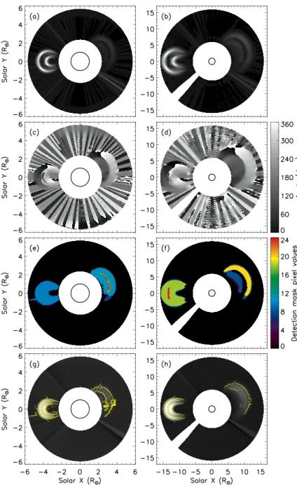
Fig. 5.— A snapshot of the algorithms applied to the model CMEs A and B. (a) and (b) show the magnitude information (edge strength), and (c) and (d) show the angular information, at a partic-ular scale of the multiscale decomposition outlined in Section 2.1. (e) and (f) show the resulting CME detection masks following the scoring system out-lined in Section 2.2. (g) and (h) show the final CME structure detection overlaid in yellow on the model C2 and C3 images. The edges were de-termined using a pixel-chaining algorithm on the magnitude and angular information of the multi-scale decomposition.
especially during solar maxima. Specifically halo CMEs (those that propagate toward or away from the observer) tend to be fainter than limb events, due to the Thomson scattering geometry and line-of-sight considerations (Vourlidas & Howard 2006;
Fig. 6.— A snapshot of the algorithms applied to the model CMEs C and D (though CME D is only visible here in the C3 image due to its later launch time than CME C). Images displayed as in Figure 5.
[image:11.612.308.525.107.452.2]the curvilinear nature of the CMEs as compared to the radial structure of the corona. The magnitude and angular information from the optimum four scales of the multiscale decomposition are used to generate the CME detection masks shown in Fig-ures 5e and 5f. In these masks the pixel values have been assigned a score corresponding to the strength of the detection (see Section 2.2). The final edge detections are over-plotted on the orig-inal model data in Figures 5g and 5h to highlight the structure in the model CMEs.
Figure 6 is displayed in the same manner as Figure 5 for a flux-rope (CME C) launched to the north-east with inclination 50◦, and a
den-sity blob (CME D) launched to the south-west alongside a relatively bright streamer region. (The timing of the events is such that CME D is only visible in the C3 image here.) The structure of the bright front of CME C is satisfactorily de-tected, while its fainter legs are indistinguishable from the background corona. In the C3 images the residual streamer material alongside CME C is included in the detection. The same is true for CME D which is detected along with the resid-ual south-west streamer material. The trailing material from the preceding passage of CME B is also present and detected at its trailing legs in the north-west and beside the top of the residual south-west streamer.
Two final blob CMEs (labelled E and F), with consecutively lower intensities than CME D, are also propagated along the same trajectory as CME D to further test the automated routines. Each of the CME blobs is also satisfactorily detected even at such low intensity levels (note from Paper I that CME F has a density only 10% that of streamers at the same height).
[image:12.612.311.524.110.227.2]In summary, the algorithm is proven to be suc-cessful at detecting each of the different model CMEs (a typical limb event, partial halo, narrow flux-rope, and small faint blobs), thus serving as a testament to its effectiveness in creating a real data catalogue. Full halo CMEs represent the lim-iting case of these events, wherein parts of the faint CME structure may not overcome the thresholds and result in disjoint or incomplete detections.
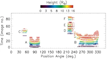
Fig. 7.— The model CME detection stack, plotted in time, i.e., image number, against position angle measured counter-clockwise from solar north. The intensity corresponds to the height of the outer-most points in the detection relative to Sun-center.
3.3. CME Model Kinematics
The model CMEs may be tested for their kinematics by investigating the detection stack that is produced from the automated algorithms. As described in Section 2.3, the detection stack is generated from the height measurements of the strongest outermost edges (along radial lines drawn from Sun-center) on the detected CME structure at each time step, i.e., for each image. It must be noted that for the model CMEs the me-dian absolute deviation threshold on the strength of the edge detections was not applied since the models are so clean (having very smooth bound-aries and minimal internal structure) that this fur-ther thresholding is not appropriate for retrieving and testing the model kinematics. It only serves as an additional step to deal with the complexity of edge detections in the real data.
For the presented model CMEs the resulting detection stack is shown in Figure 7, with time step plotted against position angle, and intensity representing height from Sun-center. Inspecting Figure 7 reveals four main detection areas: two distinct regions centered at position angles ∼90◦
and∼50◦corresponding to CMEs A and C
respec-tively; a large region spanning ∼250 – 340◦ that corresponds to CME B; and a somewhat adjoin-ing region between ∼215 – 240◦ that corresponds to the three density blobs (CMEs D, E, F) that are detected alongside the residual streamer material centered at∼240◦.
Fig. 8.— The derived velocities of CMEs A (top) and B (bottom) for each position angle of the cor-responding detections displayed in Figure 7. The velocities are shown to cluster in such a manner as to indicate an appreciable expansion of each CME, with the flanks moving slower than the apex in both cases. This is an important characteristic when considering the forces acting on a CME as it propagates.
height measurements across the complete span of angles along which the CME propagates. This results in a spread of height-time profiles that represents the different speeds attained along the expanding CME. This is an important property when considering the forces that affect CME prop-agation and expansion, especially when compared to observations further out in the corona with the Heliospheric Imagers (HI; Eyles et al. 2009), or Solar Mass Ejection Imager (SMEI; Jackson et al. 2004) for example, or indeed compared to in-situ measurements as it evolves into an interplanetary CME. Figure 8 demonstrates this capability for the relatively large flux-rope CMEs A and B. This
will allow a min, max, mean and/or median etc. velocity and acceleration to be determined, along with any changes to the position, trajectory, and angular width of the event.
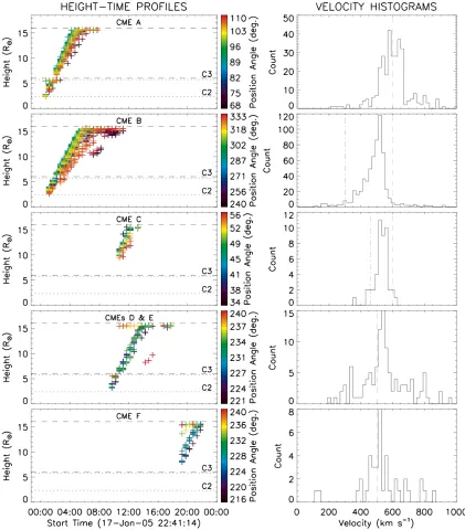
For the purposes of illustrating the automated detection technique, the above models were prop-agated with constant velocities of 600 km s−1 for
CMEs A – C and 500 km s−1 for CMEs D – F (a
model with non-constant acceleration is also dis-cussed below). Their apparent speeds are differ-ent due to the differdiffer-ent longitudinal directions of propagation (see Table 1 of Paper I). In order to retrieve the velocities of the model CMEs, the de-tection stack is inspected as follows:
1. The detection regions are cleaned and grouped as discussed in Section 2.3.
2. The height measurements along each posi-tion angle occurring in a given detecposi-tion re-gion are recorded.
3. The velocity distribution is derived using a 3-point Lagrangian interpolation on the re-sultant height-time data set.
[image:13.612.63.267.124.397.2]Note at this point that the algorithm does not fully distinguish the height-time profile of CME E from CME D, but rather determines it to be trailing material since it is detected in such close prox-imity behind CME D. This highlights the current limitation the automated methods have in sepa-rating the height measurements of co-temporal, co-spatial CMEs.
Figure 9 shows the resulting height-time mea-surements for the detection regions corresponding to CMEs A, B, C, D & E, and F, and histograms of their corresponding velocity distributions in bins of 20 km s−1. A correction, via a simple
measured velocities of CMEs B and C towards a limit of 300 and 460 km s−1 respectively. A 1σ
interval on the peak of each of the velocity distri-butions overlaps the known model velocity, even for the CMEs suffering projection effects. Thus, it is deemed that the automated detection and track-ing techniques satisfactorily determine the correct height-time profiles of the models, thereby verify-ing their applicability and robustness.
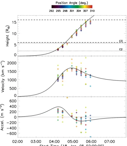
Another model CME flux-rope was generated to test how the automated methods would fare with regards to deriving a non-constant acceler-ation profile, specifically one which exhibits an initial peak followed by a deceleration and then leveling to zero. This is akin to a general impul-sive CME that undergoes an initial high accelera-tion and then decelerates to match the solar wind speed. The model kinematic profiles are described by the following equations, based on a variation of the acceleration function chosen by Gallagher et al. (2003):
h(t) = √2x ttan−1e√t/2x
2x
(9)
v(t) = √2xtan−1e√t/2x
2x
+ et/2xt
et/x+2x (10)
a(t) = e
t/2x(2x(t+4x)−et/x(t−4x))
2x(et/x+2x)2 (11)
where xis a scaling factor, set at x= 1200 for this case. Figure 10 shows the model CME kine-matics (solid line) and the over-plotted height, velocity, and acceleration measurements result-ing from the CORIMP automated detection and tracking of the CME. The 3-point Lagrangian in-terpolation is prone to some scatter, especially at the end-points which are therefore less reliable. The kinematic trends of the model CME are, how-ever, satisfactorily revealed by the methods. It is clear that the limits of the observations (restricted fields-of-view, cadence, measurement errors) can dramatically affect their derivation. For example, there are only two satisfactory measurements in C2 before the majority of the CME front leaves the field-of-view, and similarly for the final mea-surement in C3 where some of the CME front has already left the field-of-view. Nonetheless, given these inherent limitations of the data, the auto-mated methods still prove accurate and effective.
[image:15.612.310.520.146.386.2]Ongoing efforts in this vein will lead to a cat-alogue of real data that can list the determined
Fig. 10.— A non-constant acceleration profile in-put to a model flux-rope CME, and the resulting derived kinematics from the CORIMP automated detection algorithms. The solid curves are the model kinematics, and the ‘plus’ symbols are the resulting kinematics from the automated detection algorithms with a colorbar indicating their rele-vant position angles (measured counter-clockwise from solar north).
4. Conclusions
The main objective in implementing an auto-mated detection and tracking routine is to out-put reproducible, robust, accurate CME measure-ments (height, width, position angle, etc.). Cur-rent methods of CME detection have their limita-tions, mostly since these diffuse objects have been difficult to identify using traditional image pro-cessing techniques. These difficulties arise from the transient nature of the CME morphology, the scattering effects and non-linear intensity profile of the surrounding corona, the presence of coro-nal streamers, and the addition of noise due to cosmic rays and solar energetic particles (SEPs) that impact the coronagraph detector, along with instrumental effects of stray light, the limitations imposed by low cadence observations, and data corruption or dropouts. In the introduction to this paper, the drawbacks of current cataloguing pro-cedures for investigating CME dynamics (CDAW, CACTus, SEEDS, ARTEMIS) were highlighted as the motivation for establishing a new cata-logue. However, given the highly variable nature of CME phenomena and the coronal atmosphere they traverse, there are certain limitations that can never be overcome but only minimized; and it is exactly such a minimizing of current limita-tions that these new CORIMP methods achieve. The methods are completely automated, mak-ing them robust and reproducible - important for back-dating the full LASCO dataset and inspect-ing the statistics across thousands of events. The automated detection has been extended through both the LASCO/C2 and C3 fields-of-view with-out any need for differencing, thus minimizing the issues of under-sampling events and of the uncer-tainty involved when subtracting and scaling im-ages. The multiscale filtering technique reveals the CME structure and so minimizes the uncertainty in determining their often complex geometry. The number of scales in the multiscale decomposition also allows a strength of detection to be assigned through both the magnitude and angular infor-mation, thus minimizing the chances that a CME, or parts thereof, go undetected. Furthermore, the spread of measurements available for inspection of the CME kinematics minimizes the uncertainty involved when deriving velocity and acceleration profiles, which is important for comparing with physical theory of CME propagation. Indeed, the
overall CORIMP method of automatically detect-ing, trackdetect-ing, and deriving CME parameters has been described and demonstrated here on a num-ber of well-conceived models, and real data, with excellent results.
This work is supported by SHINE grant 0962716 and NASA grant NNX08AJ07G to the Institute for Astronomy. We thank the anonymous referee for their valuable comments. The SOHO/LASCO data used here are produced by a consortium of the Naval Research Laboratory (USA), Max-Planck-Institut fuer Aeronomie (Germany), Lab-oratoire d’Astronomie (France), and the Univer-sity of Birmingham (UK). SOHO is a project of international cooperation between ESA and NASA. The STEREO/SECCHI project is an in-ternational consortium of the Naval Research Laboratory (USA), Lockheed Martin Solar and Astrophysics Lab (USA), NASA Goddard Space Flight Center (USA), Rutherford Appleton Lab-oratory (UK), University of Birmingham (UK), Max-Planck-Institut f¨ur Sonnen-systemforschung (Germany), Centre Spatial de Liege (Belgium), In-stitut d’Optique Th´eorique et Appliqu´ee (France), and Institut d’Astrophysique Spatiale (France).
REFERENCES
Boursier, Y., Lamy, P., Llebaria, A., Goudail, F., & Robelus, S. 2009, Sol. Phys., 257, 125
Brueckner, G. E., Howard, R. A., Koomen, M. J., et al. 1995, Sol. Phys., 162, 357
Byrne, J. P., Gallagher, P. T., McAteer, R. T. J., & Young, C. A. 2009, A&A, 495, 325
Byrne, J. P., Maloney, S. A., McAteer, R. T. J., Refojo, J. M., & Gallagher, P. T. 2010, Nature Communications, 1
Chen, J., & Krall, J. 2003, Journal of Geophysical Research (Space Physics), 108, 1410
Chen, P. F. 2011, Living Reviews in Solar Physics, 8, 1
dal Lago, A., Schwenn, R., & Gonzalez, W. D. 2003, Advances in Space Research, 32, 2637
Emslie, A. G., Kucharek, H., Dennis, B. R., et al. 2004, Journal of Geophysical Research (Space Physics), 109, 10104
Eyles, C. J., Harrison, R. A., Davis, C. J., et al. 2009, Sol. Phys., 254, 387
Gallagher, P. T., Lawrence, G. R., & Dennis, B. R. 2003, ApJ, 588, L53
Gallagher, P. T., Young, C. A., Byrne, J. P., & McAteer, R. T. J. 2011, Advances in Space Re-search, 47, 2118
Gopalswamy, N., & Kundu, M. R. 1992, ApJ, 390, L37
Gopalswamy, N., Lara, A., Lepping, R. P., et al. 2000, Geophys. Res. Lett., 27, 145
Gopalswamy, N., Yashiro, S., Kaiser, M. L., Howard, R. A., & Bougeret, J.-L. 2001, Journal of Geophysics Research, 106, 29219
Gopalswamy, N., Yashiro, S., Michalek, G., et al. 2009, Earth Moon and Planets, 104, 295
Howard, R. A., Moses, J. D., Vourlidas, A., et al. 2008, Space Science Reviews, 136, 67
Howard, T. A., & Tappin, S. J. 2009, Space Sci-ence Reviews, 147, 31
Hudson, H. S., Acton, L. W., & Freeland, S. L. 1996, ApJ, 470, 629
Illing, R. M. E., & Hundhausen, A. J. 1985, J. Geophys. Res., 90, 275
Jackson, B. V. 1985, Sol. Phys., 100, 563
Jackson, B. V., Buffington, A., Hick, P. P., et al. 2004, Sol. Phys., 225, 177
Kaiser, M. L., Kucera, T. A., Davila, J. M., et al. 2008, Space Science Reviews, 136, 5
Kliem, B., & T¨or¨ok, T. 2006, Physical Review Let-ters, 96, 255002
Klimchuk, J. A. 2001, Space Weather (Geophys-ical Monograph 125), ed. P. Song, H. Singer, G. Siscoe (Washington: Am. Geophys. Un.), 125, 143
Lepping, R. P., Berdichevsky, D. B., Szabo, A., Arqueros, C., & Lazarus, A. J. 2003, Sol. Phys., 212, 425
Lockwood, M., & Hapgood, M. 2007, Astronomy and Geophysics, 48, 060000
Lynch, B. J., Antiochos, S. K., DeVore, C. R., Luhmann, J. G., & Zurbuchen, T. H. 2008, ApJ, 683, 1192
Maloney, S. A., Gallagher, P. T., & McAteer, R. T. J. 2009, Sol. Phys., 256, 149
Martens, P. C. H., Attrill, G. D. R., Davey, A. R., et al. 2012, Sol. Phys., 275, 79
Moon, Y.-J., Choe, G. S., Wang, H., et al. 2002, ApJ, 581, 694
Morgan, H., Byrne, J. P., & Habbal, S. R. 2012, ApJ, 752, 144
Morgan, H., & Habbal, S. 2010, ApJ, 711, 631
Morgan, H., Habbal, S. R., & Lugaz, N. 2009, ApJ, 690, 1119
Morgan, H., Habbal, S. R., & Woo, R. 2006, Sol. Phys., 236, 263
Olmedo, O., Zhang, J., Wechsler, H., Poland, A., & Borne, K. 2008, Sol. Phys., 248, 485
P´erez-Su´arez, D., Higgins, P. A., Bloomfield, D. S., et al. 2011, “Automated Solar Feature Detection for Space Weather Applications”, in Applied Signal and Image Processing: Multi-disciplinary Advancements, eds. R. Qahwaji, R. Green, & E. L. Hines, (IGI Global), p. 207 – 225
Priest, E. R., & Forbes, T. G. 2002, A&A Rev., 10, 313
Robbrecht, E., & Berghmans, D. 2004, A&A, 425, 1097
Robbrecht, E., Patsourakos, S., & Vourlidas, A. 2009, ApJ, 701, 283
Schwenn, R., dal Lago, A., Huttunen, E., & Gon-zalez, W. D. 2005, Annales Geophysicae, 23, 1033
Temmer, M., Veronig, A. M., Kontar, E. P., Krucker, S., & Vrˇsnak, B. 2010, ApJ, 712, 1410
Tousey, R., & Koomen, M. 1972, in Bulletin of the American Astronomical Society, 4, 394
Vourlidas, A., & Howard, R. A. 2006, ApJ, 642, 1216
Webb, D. F., & Howard, T. A. 2012, Living Re-views in Solar Physics,submitted.
Yashiro, S., Gopalswamy, N., Michalek, G., et al. 2004, Journal of Geophysical Research (Space Physics), 109, 7105
Young, C. A., & Gallagher, P. T. 2008, Sol. Phys., 248, 457
Zhang, J., & Dere, K. P. 2006, ApJ, 649, 1100
Zhang, J., & Wang, J. 2002, ApJ, 566, L117
This 2-column preprint was prepared with the AAS LATEX