A Numerical Simulation of a Three-dimensional
Air Quality Model in an Area Under a Bangkok
Sky Train Platform Using an Explicit Finite
Difference Scheme
Kewalee Suebyat, Nopparat Pochai
Abstract—One of the air pollution problems in areas under Bangkok sky train platforms are caused by the pollutant coming from the entrance to the tunnel. It increases the concentration of pollutant. This affects the well-being of humans and the environment. In this research, the governing equation of the air quality model in a considered area is a three-dimensional advection-diffusion equation with time dependence. A finite difference technique is employed to approximate the solution of the governing equation. This model is solved by using an explicit forward difference in time and central difference in space (FTCS). We consider the wind inflow in two cases: there is wind inflow only inx-direction and there are wind inflow inx -direction andy-direction. In addition, we added obstacles such as the columns along the middle into the tunnel. The results of the model are satisfactory. It will be able to be implemented on a problem of air pollution control in a more complicated tunnel.
Index Terms—air quality, advection-diffusion equation, finite difference method, FTCS, Bangkok sky train, tunnel.
I. INTRODUCTION
A
IR pollution is a global problem for human life and environment that should be realized. It comes from many sources such as forest fires, industrial factory area, traffic jam and more, especially, an area under Sky Train of the Bangkok Transit System (BTS). It provides an effective route of urban transport for people of Bangkok because BTS facilitates quick and easy transportation. However, it is also causing some of the environmental impacts especially the air pollutant impact to the vicinity area around its platform with heavy traffic and a lot of people. The major source of air pollution under Bangkok sky train platform comes from vehicle exhaust, mobile source and others sources including commercial, smoke from the store, construction and building demolition. The air pollutants emitted from mobile source are Carbon Monoxide (CO) and Nitrogen Oxides (NOx). CO is a product of incomplete combustion of fuel such as natural gas, coal or wood. Vehicular exhaust is a major source of carbon monoxide. In areas of high vehicle traffic, such as in large cities, NOx emitted can be a significant source of air pollution. It raises the earth's temperature and becomes air pollutants. Their concentration levels cause injury to human health and an harmful for survival. The effects of air pollutionManuscript received May 02, 2017; revised September 14, 2017. Kewalee Suebyat and Nopparat Pochai are with Department of Mathemat-ics, Faculty of Science, King Mongkuts Institute of Technology Ladkrabang, Bangkok 10520, Thailand and Centre of Excellence in Mathematics, Com-mission on Higher Education (CHE), Si Ayutthaya Road, Bangkok 10400, Thailand. Email: kew26 [email protected] and nop [email protected].
are alarming. Several people are known to have died due to direct or indirect effect of air pollution. It is known that air pollution contributes to cancer among other threats to the body.
Nowadays, there are heavy traffic and an increase in population. It’s the cause of air pollution on the road. Air pollution around the platform in an area under Bangkok sky train platform has increased greatly, so it is interesting to study. However this area should be implemented into the wind inflow direction near the tunnel because it affects the concentration of air pollutant. Then the wind inflow is an important factor of the model.
In 1961, [1] studied the pollution of the air by motor vehi-cles, measurements were made in two London road tunnels during periods of high traffic density. The concentrations of smoke and polycyclic hydrocarbons found that there were much higher than the average values in Central London, but they were of the same order of magnitude as those occurring during temperature inversions on winter evenings when smoke from coal fires accumulates at a low level. In 2004, [2] defined and calculated the stability conditions for several numerical methods for a three-dimensional advection-diffusion equation and compared the numerical solutions. In 2008, [3] presented the modification of Krylov Subspace Spectral (KSS) methods by using the Lanczos iteration to computed the quadrature rules. KSS methods were second-order accurate and unconditionally stable. For more than one node are shown to possess favorable stability proper-ties as well. In 2010, [4] presented a new Pad numerical scheme for the solution of two-dimensional diffusion equa-tions with nonlocal boundary condiequa-tions on four boundaries. The numerical results are shown that these Pad schemes are efficient and provided very accurate results. In 2010, [5] studied a three dimensional advection-diffusion equation of air pollutant is applied to a street tunnel configuration. In 2011, [6] studied a mathematical model of the smoke dispersion from two sources and one source with a structural obstacle was considered. In 2013, [7] studied and compared the performance of 3 different CFD numerical approaches, namely RANS, URANS and LES for evaluation to deter-mine suitability in the prediction of air flow and pollutant dispersion in urban street canyons. The results showed that LES was observed to produce accurate more than RANS and URANS. In 2015, [8] developed the Fluctuating Wind Boundary Conditions (FWBC) and compared to SWBC in order to determine suitability in the investigation of air flow and pollutant dispersion in urban street canyons. 3D
numer-IAENG International Journal of Applied Mathematics, 47:4, IJAM_47_4_16
Fig. 1. The steet tunnel configuration.
ical simulations are performed using Large Eddy Simulation (LES). The FWBC has produced more realistic results when compared to the frequently employed SWBC. In 2015, [9] calculated the concentration of air pollutant and to assessed the air quality state all over the Region. The analysis was carried out by using the Gaussian model ISC. This modeling approach can be considered as an important assessment tool for the local environmental authorities in Campania region, Southern Italy. In 2016, [10] studied a mathematical model for describing the dispersion of the air pollutants released from the source into the atmosphere was examined by using the three-dimensional fractional step method. The results obtained indicated that the proposed experimental variations of the atmospheric stability classes and wind velocities did affect the air quality around the industrial areas. In 2016, [11] studied and presented the development of a next generation air sensor system and application in anad hocair monitoring network, in which the air sensors were placed and operated at the street level to monitor the air along the Marathon route in urban Hong Kong and the near-real time calculation and communication of health-indexed findings of air quality to the public.
The purpose of this paper is to approximate the concentra-tion of air pollutant in two cases: there is wind inflow only in
x-direction and there are wind inflow inx- andy-directions by using the finite difference technique.
II. GOVERNINGEQUATION
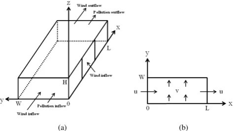
The tunnel is an underground passageway with is enclosed except for the entrance and exit. In this paper, the configura-tion of the area street tunnel is shown in Fig. 1. That is, above the street is sky train platform and both sides of the street are section of buildings. The simulation of configuration of street tunnel are divided into two cases: Case 1: we assume that there is wind inflow only in x-direction. The domain for street tunnel in Case 1 is shown in Fig. 2(a) and the wind direction in this case is shown in Fig. 2(b). Case 2: we assume that there are wind inflow inx- andy-directions. The domain for street tunnel in Case 2 is shown in Fig. 3(a) and the wind direction in this case is shown in Fig. 3(b). Then the consider domain becomes: Ω ={(x, y, z); 0 ≤x≤L, 0 ≤ y ≤ W, 0 ≤ z ≤ H}, where W is the width (m),
L is the length (m) and H is the height (m) of the street tunnel. The air pollutant concentration can be described by the advection-diffusion equation following:
∂C
∂t +V · 5C=5 ·
¯
K⊗ 5C
, (1)
(a) (b)
Fig. 2. (a) The domain for street tunnel (Case 1). (b) The wind direction (Case 1).
(a) (b)
Fig. 3. (a) The domain for street tunnel (Case 2). (b) The wind direction (Case 2).
whereC=C(x, y, z, t) is the air pollutant concentration at (x, y, z)and timet(kg/m3),5= ∂
∂x~i+ ∂ ∂y~j+
∂
∂z~k, and⊗is
matrix multiplication. The vectorV is the wind velocity field (m/sec) and K¯ is the eddy-diffusivity or dispersion tensor (m2/sec).
By the assumption, we assumed that the wind inflow is horizontal direction. We shall consider the three-dimensional advection-diffusion equation in Eq. (1), which can be written as:
∂C ∂t +u
∂C ∂x +v
∂C ∂y =Dh
∂2C
∂x2 +Dh
∂2C
∂y2 +Dv
∂2C
∂z2, (2)
where u is a constant wind velocity in the x-direction (m/sec), v is a constant wind velocity in the y-direction (m/sec),Dh is a constant dispersion coefficient in the
hor-izontal direction (m2/sec) and D
v is a constant dispersion
coefficient in the the z-direction (vertical) (m2/sec) appropri-ate initial and boundary conditions. When we consider the components of the tunnel, it is shown in Fig. 4. The initial condition is assumed by the cold start technique that the air pollutant concentration is to be zero in the whole domain. It is obtained that
C(x, y, z,0) = 0, (3)
for all 0 ≤ x ≤ L, 0 ≤ y ≤ W, 0 ≤ z ≤ H. For the boundary conditions, we distinguish three different cases in the considered domain as following:
Case I: assuming that there is the wind inflows in x -direction. In Fig. 5, model of the Case I is shown.
IAENG International Journal of Applied Mathematics, 47:4, IJAM_47_4_16
[image:2.595.311.550.62.197.2] [image:2.595.307.545.250.383.2]Fig. 4. Components of the tunnel.
Entrance gate :C(0, y, z, t) =c1. Exit gate : ∂C∂x(L, y, z, t) =c2. Side walls : ∂C∂y(x,0, z, t) = ∂C
∂y(x, W, z, t) = 0.
Ground : ∂C∂z(x, y,0, t) = 0.
Platform ceiling : ∂C∂z(x, y, H, t) = 0, A < y < B.
Parallel gap : ∂C∂z(x, y, H, t) =c3,otherwise, where c1 is the inflow air pollutant concentration in x -direction, c2 is the average rate of change of air pollutant concentration at the exit gate,c3is the average rate of change of air pollutant concentration along the both parallel gap, A
is the right parallel gap size along the ceiling, and B is the left parallel gap size along the ceiling.
Case II: assuming that there are the obstacles as the platform column. For the model in this case shown in Fig.6.
Entrance gate :C(0, y, z, t) =c1. Exit gate : ∂C∂x(L, y, z, t) =c2. Side walls : ∂C∂y(x,0, z, t) = ∂C
∂y(x, W, z, t) = 0.
Ground : ∂C∂z(x, y,0, t) = 0.
Platform ceiling : ∂C∂z(x, y, H, t) = 0, A < y < B.
Parallel gap : ∂C∂z(x, y, H, t) =c3,otherwise. Center column :C(Di, E, z, t) = 0,0≤z≤H.
Front and back column : ∂C∂x(Di−1, y, z, t) = ∂C∂x(Di
+1, y, z, t) = 0, E−1≤y ≤E+ 1;t >0.
Left and right column : ∂C∂y(x, E−1, z, t) = ∂C ∂y(x, E
+1, z, t) = 0, Di−1≤x≤Di+ 1;t >0,
where (Di, E)is a center point of the platform column in x- and y-directions, for i= 1,2, ..., ncl,ncl is the number of platform column.
Case III: assuming that there are the wind inflow in x -andy-directions. In Fig. 7, model of the Case III is shown.
Entrance gate :C(0, y, z, t) =c1. Exit gate : ∂C∂x(L, y, z, t) =c2. Ground : ∂C∂z(x, y,0, t) = 0.
Platform ceiling : ∂C∂z(x, y, H, t) = 0, A < y < B.
Parallel gap : ∂C∂z(x, y, H, t) =c3,otherwise. Left side wall : ∂C∂y(x, W, z, t) = 0.
Right side wall gap : C(x,0, z, t) =c4, F ≤x≤G, 0≤z≤H.
Right side wall : ∂C∂y(x,0, z, t) = 0,otherwise, where c4 is the inflow air pollutant concentration in y -direction andF−Gis the side wall gap of the beside consider domain.
III. NUMERICALTECHNIQUES
[image:3.595.72.271.58.159.2]We use the finite difference method for approximating the solution of the three-dimensional advection-diffusion equation. The solution domain of the problem over a time 0≤t≤T is covered by a mesh of grid-lines:xi=i∆x, i=
Fig. 5. Model of the Case I.
[image:3.595.305.548.589.791.2]Fig. 6. Model of the Case II.
Fig. 7. Model of the Case III.
0,1,2, ..., M;yj = j∆y, j = 0,1,2, ..., N;zk =k∆z, k =
0,1,2, ..., O;tn = n∆t, n = 0,1,2, ..., R; parallel to the
space and time coordinate axes, respectively. Approximations
Cn
i,j,ktoC(i∆x, j∆y, k∆z, n∆t)are calculated at the point
of intersection of these lines, namely,(i∆x, j∆y, k∆z, n∆t) which is referred to as the(i, j, k, n)grid point. The constant spatial and temporal grid-spacing are ∆x = ML,∆y =
W N,∆z=
H O,∆t=
T
R, respectively.
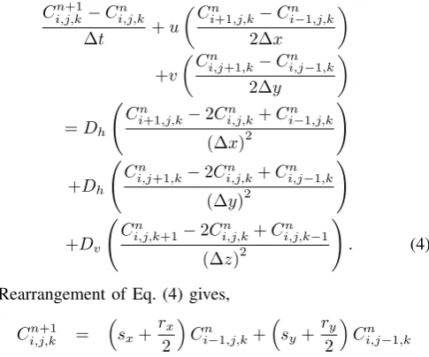
In this paper, we use an explicit forward-difference approximation for the time-derivative (FT), and central-difference approximations for the space-derivatives (CS). It is called FTCS. The approximate solution of the governing equation uses the finite difference scheme satisfies:
Ci,j,kn+1−Cn i,j,k
∆t +u
Cn
i+1,j,k−C n i−1,j,k
2∆x
+v
Cn
i,j+1,k−C n i,j−1,k
2∆y
=Dh Cn
i+1,j,k−2C n i,j,k+C
n i−1,j,k
(∆x)2
!
+Dh
Ci,jn+1,k−2Ci,j,kn +Ci,jn−1,k
(∆y)2
!
+Dv Cn
i,j,k+1−2Ci,j,kn +Ci,j,kn −1
(∆z)2
!
. (4)
Rearrangement of Eq. (4) gives,
Ci,j,kn+1 = sx+ rx
2
Cin−1,j,k+sy+ ry
2
Ci,jn−1,k
IAENG International Journal of Applied Mathematics, 47:4, IJAM_47_4_16
+ (sz)Ci,j,kn −1+
sx− rx
2
Cin+1,j,k
+ sy− ry
2
Ci,jn+1,k+ (sz)Ci,j,kn +1
+ (1−2sx−2sy−2sz)Ci,j,kn , (5)
in whichrx = u∆∆xt, ry = v∆∆yt, sx= (∆Dhx∆)2t, sy = (∆Dhy∆)2t and
sz = (∆Dvz∆)2t. The stability of this three-dimensional finite difference method may be investigated by using the von Neumann method shows that [2], [12] are stable if both
sx+sy+sz≤
1
2, (6)
and
r2x sx
+r 2 y sy
≤3, (7)
are satisfied. The finite difference scheme for the left-hand side (x= 0)and the right-hand side(x=L)as following:
∂C
∂x(x0, yj, zk)≈
−3C0n,j,k+ 4C1n,j,k−C2n,j,k
2∆x , (8)
∂C
∂x(xM, yj, zk)≈
3Cn
M,j,k−4C n
M−1,j,k+C n M−2,j,k
2∆x , (9)
respectively. Iny- andz- directions are obtained in the same way.
IV. NUMERICALEXPERIMENTS
In this section, we will show 3 cases as already mentioned in the previous section, i.e. an area under Sky Train of the Bangkok Transit System (BTS). For Case I and Case II, we assume that there is wind inflow only in x-direction. Case II is similar to Case I, but we add the boundary conditions of obstacles in the tunnel. For Case III, we assume that there are wind inflow in x- and y-directions. We consider the length, width and height of tunnel are 192, 26 and 6 meters, respectively. Then, the problem domain is Ω ={(x, y, z); 0≤x≤192,0≤y≤26,0≤z≤6}.
Case I: for more realistic problem, the parallel gaps along the tunnel between the ceiling and their building of the both sides are added in to the domain. It is assumed that the rate of change are decreased at the parallel gaps and the exit gate. We consider the three-dimensional advection-diffusion equation in Eq. (2) and we assume that c1 = 1,c2=c3= −0.01,A= 4,B= 24.
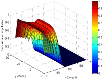
The numerical results of Case I are shown in Table I and Figs. 8-11. Fig. 8 and Fig. 9 show the air pollutant concentration levels after passed 30 second in contour plot and surface plot, respectively. Fig. 10 and Fig. 11 show the air pollutant concentration levels after 120 second has passed in contour plot and surface plot, respectively.
Those figures show the numerical solutions in Case I, where∆x= ∆y= ∆z= 2m;∆t= 0.06sec;Dh= 0.1592
m2/sec; D
v = 0.05 m2/sec; u= 2.7778m/sec; v = 0m/sec; z = 4 m. If we take more time into our system, the concentration of pollutant will be reduce as well.
Case II: in reality, there are obstacles such as columns. So, we will add the boundary conditions of obstacles in the tun-nel. It is assumed that no rate of change at the columns. We consider the three-dimensional advection-diffusion equation in Eq. (2) and we assume that c1 = 1, c2 =c3 = −0.01,
A= 4,B= 24,D1= 41,D2= 101,D3= 161,E= 14.
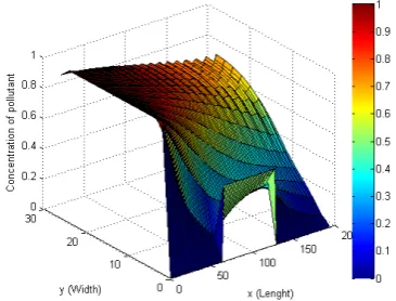
The numerical results of Case II are shown in Table II and Figs. 12-15. Fig. 12 and Fig. 13 show the air pollutant concentration levels after passed 30 second in contour plot and surface plot, respectively. Fig. 14 and Fig. 15 show the air pollutant concentration levels after 120 second has passed in contour plot and surface plot, respectively.
Those figures show the numerical solutions in Case II where∆x= ∆y= ∆z= 1m;∆t= 0.06sec;Dh= 0.1592
m2/sec;Dv = 0.05m2/sec;u= 2.7778m/sec;v= 0m/sec; z = 4 m. The results are agreeable, the concentration of pollutant are decreased away from the source.
Case III: in this example, we consider the wind inflow inx -andy-directions. That is, we will adduinx-direction andv
iny-direction. We consider the three-dimensional advection-diffusion equation in Eq. (2) and we assumec1 = 1,c2 =
c3=−0.01,c4= 0.5,A= 4, B= 24,F = 64,G= 129. The numerical results of Case III are shown in Table III and Figs. 16-19. Fig. 16 and Fig. 17 show the air pollutant concentration levels after passed 30 second in contour plot and surface plot, respectively. Fig. 18 and Fig. 19 show the air pollutant concentration levels after 120 second has passed in contour plot and surface plot, respectively.
Those figures show the numerical solutions in Case III, where∆x= ∆y= ∆z= 2m;∆t= 0.06sec;Dh= 0.1592
m2/sec; Dv = 0.05 m2/sec; u = 2.7778 m/sec; v = 20u
m/sec; z = 4 m. The results are reasonable, the calculated of pollutant are decreased away from the source.
V. CONCLUSION
The proposed model can be used to measure air pollutant concentration in a partly opened street tunnel, especially, an area under Bangkok sky train platform. The model is gov-erned by a three-dimensional in space and one-dimensional in time of the advection-diffusion equation. The results from 3 cases can be summarized as follows: if we take a long time, it can be seen that the concentration of air pollutant has decreased even though the distance has increased. That is, the concentration varied with the length of distance. The results are satisfactory because there is no outside air flow. Then, there is the wind inflow only inx-direction from the entrance gate into the tunnel. However, we added obstacles into the tunnel such as the columns along the middle. As results, the concentration of air pollutant has increased, especially the front of columns has a higher concentration than the back of columns. The higher of air pollution comes from the columns. Furthermore, there are the wind inflow inx- and
y-directions. We assume that the sources are emitted from the entrance gate and the right side wall gap. It caused the concentration of pollution in the left side wall to be higher than other areas. The boundary conditions are not limited only to constant functions but can be assumed to have several interpolated functions. The proposed explicit finite difference method gives a good agreement and reasonable results. Furthermore, the implicit method that unconditionally stable should be introduced as well.
ACKNOWLEDGMENT
This paper is supported by the Centre of Excellence in Mathematics Program of the Commission on Higher Education (CEM), Thailand. The authors greatly appreciate valuable comments received from the reviewers.
IAENG International Journal of Applied Mathematics, 47:4, IJAM_47_4_16
Table. I. The air pollutant concentration for Case I at z= 4 m and T = 30sec.
y(m)\x(m) 30 60 90 120 150
6 0.8949 0.6173 0.0390 -0.0005 -0.0010 10 0.9278 0.6704 0.0454 -0.0001 -0.0006 14 0.9288 0.6727 0.0460 -0.0000 -0.0004 18 0.9287 0.6724 0.0459 -0.0000 -0.0005 22 0.9229 0.6599 0.0436 -0.0003 -0.0009
Table. II. The air pollutant concentration for Case II atz= 4 m and T = 30sec.
y(m)\x(m) 30 60 90 120 150
6 0.9435 0.7615 0.0165 -0.0001 -0.0001 10 0.9353 0.6499 0.0131 -0.0000 -0.0000 14 0.8718 0.2665 0.0085 -0.0000 -0.0000 18 0.9432 0.7561 0.0161 -0.0000 -0.0000 22 0.9406 0.7469 0.0152 -0.0003 -0.0003
Table. III. The air pollutant concentration for Case III at
z= 4m and T = 30sec.
y(m)\x(m) 30 60 90 120 150
6 0.7350 0.3842 0.0936 0.1909 0.2055
10 0.9141 0.6336 0.0417 0.0284 0.0653 14 0.9278 0.6710 0.0451 0.0021 0.0083 18 0.9288 0.6727 0.0460 0.0001 0.0002 22 0.9287 0.6725 0.0458 -0.0001 -0.0006
REFERENCES
[1] R. E. Waller, B. T. Commins and P. J. Lawther, “Air pollution in road tunnels,”Brit. J. industr. Med., vol. 18, pp. 250, 1961.
[2] M. Dehghan, “Numerical solution of the three-dimensional advection diffusion equation,”Applied Mathematics and Computation, vol. 150, pp. 5-19, 2004.
[3] J. V. Lambers, “An explicit, stable, highorder spectral method for the wave equation based on block gaussian quadrature,”IAENG Interna-tional Journal of Applied Mathematics, vol. 38, no. 4, pp. 233-248, 2008.
[4] M. Siddique, “Numerical computation of two-dimensional diffusion equation with nonlocal boundary conditions,” IAENG International Journal of Applied Mathematics, vol. 40, no. 1, pp. 26-31, 2010. [5] M. Thongmoon, “Numerical experiment of air pollutant concentration
in the street tunnel,”International Mathematical Forum, vol. 10, pp. 449-465, 2010.
[6] N. Pochai, “A finite element solution of the mathematical model for smoke dispersion from two sources,”World Academy of Science, Engineering and Technology, vol. 60, pp. 1691-1695, 2011.
[7] S. M. Salim and K. C. Ong, “Performance of RANS, URANS and LES in the prediction of airflow and pollutant dispersion,” IAENG Transactions on Engineering Technologies: Lecture Notes in Electrical Engineering, vol. 170, pp. 263-274, 2013.
[8] S. M. Kwa and S. M. Salim, “Numerical simulation of dispersion in an urban street canyon: comparison between steady and fluctuating boundary conditions,” Engineering Letters, vol. 23, no.1, pp. 55-64, 2015.
[9] P. Iodice and A. Senatore, “Environmental assessment of a wide area under surveillance with different air pollution sources,” Engineering Letters, vol. 23, no.3, pp. 156-162, 2015.
[10] S. A. Konglok and N. M. Pochai, “Numerical computations of three-dimensional air-Quality model with variations on atmospheric stability classes and wind velocities using fractional step method,” IAENG International Journal of Applied Mathematics, vol. 46, no.1, pp. 112-120, 2016.
[11] L. Sun, K. C. Wong, P. Wei, S. Ye, H. Huang, F. Yang, D. Westerdahl, K. K. Louie, W. Y. Luk, and Z. Ning, “Development and application of a next generation air sensor network for the Hong Kong marathon 2015 air quality monitoring,” inLecture Notes in Engineering and Computer Science: Sensors, vol. 16, pp. 211, 2016.
[image:5.595.336.516.243.381.2][12] A. C. Hindmarsh, P. M. Gresho, and D. F. Griffiths, “The stability of explicit euler time-integration for certain finite difference approxima-tions of the multi-dimensional advection-diffusion equation,” innt. J. Numer. Methods Fluids, vol. 4, pp. 853-897, 1984.
[image:5.595.337.517.427.568.2]Fig. 8. Contour plot of concentration of air pollutant levels for Case I after passed 30 second.
[image:5.595.336.516.615.753.2]Fig. 9. Surface plot of concentration of air pollutant levels for Case I after passed 30 second.
Fig. 10. Contour plot of concentration of air pollutant levels for Case I after passed 120 second.
Fig. 11. Surface plot of concentration of air pollutant levels for Case I after passed 120 second.
IAENG International Journal of Applied Mathematics, 47:4, IJAM_47_4_16
Fig. 12. Contour plot of concentration of air pollutant levels for Case II after passed 30 second.
[image:6.595.336.517.244.381.2]Fig. 13. Surface plot of concentration of air pollutant levels for Case II after passed 30 second.
Fig. 14. Contour plot of concentration of air pollutant levels for Case II after passed 120 second.
[image:6.595.81.264.245.384.2]Fig. 15. Surface plot of concentration of air pollutant levels for Case II after passed 120 second.
[image:6.595.336.517.424.569.2]Fig. 16. Contour plot of concentration of air pollutant levels for Case III after passed 30 second.
Fig. 17. Surface plot of concentration of air pollutant levels for Case III after passed 30 second.
Fig. 18. Contour plot of concentration of air pollutant levels for Case III after passed 120 second.
Fig. 19. Surface plot of concentration of air pollutant levels for Case III after passed 120 second.