Empty Containers Inventory System with Fuzzy Demand

ABSTRACT – In this research, with the trend of globalization; trade inequality leads to differences in the throughput of ports. Ports with large number of export goods will face the problem of the lacking of containers. In the model, the cost of dispatching containers is divided into three parts: container holding cost, container ordering cost and container leasing cost. According to the status of inventory level, cost can be effectively reduced according to which method is used to dispatch the container. Due to the reason of demand for each period cannot be accurately predicted, therefore fuzzy theory is added in the research in order to obtain a more realistic and accurate result. Finally, this research cooperates Matlab R2014b in calculating the result for the hypothesis model.

Index Terms—Trade inequality, empty containers scheduling, fuzzy theory

I. INTRODUCTION

s a low-cost, high-capacity transport vehicle, shipping is definitely an important and indispensable means of trade in international trade. For shipping, cost is the primary consideration. The import and export volume of each port is different. If there are more ports than imported ports, there will be problems with excessive containers; if ports with less imports than exports, there will be a shortage of containers. For ports that are out of the containers, the cost of container dispatching is a challenge. If there is a set of well-considered models, the cost can be effectively controlled.

Yang M.F. (2006) uses fuzzy theory to create fuzzy assumptions about the integration of inventory model demand and productivity, also uses the reduced distance method to estimate the total cost. During the process of fuzzification and defuzzification, each procedure is described in detail.

Manuscript received November 28, 2018; revised December 05, 2018. This work was supported in part by the Department of Transportation Science, National Taiwan Ocean University. Paper title is Empty Containers Inventory System with Fuzzy Demand (paper number: ICOR_7). C. H Lin Author is with the department of transportation science, National Taiwan Ocean University, No.2, Beining Rd., Keelung City 202, Taiwan (R.O.C), (corresponding author to provide phone: 0926-188-797; e-mail: [email protected])

C. M. Su Author is with Center of Excellence for Ocean Engineering; the department of transportation science, National Taiwan Ocean University, No.2, Beining Rd., Keelung City 202, Taiwan (R.O.C), (e-mail: [email protected])

S. L. Kao Author is with Center of Excellence for Ocean Engineering; the department of transportation science, National Taiwan Ocean University, No.2, Beining Rd., Keelung City 202, Taiwan (R.O.C). (e-mail: [email protected])

M. F. Yang Author is with Center of Excellence for Ocean Engineering; the department of transportation science, National Taiwan Ocean University, No.2, Beining Rd., Keelung City 202, Taiwan (R.O.C), (e-mail: [email protected])

Rafael Diaz et al. (2011) compared the number of empty containers in the port to a more cost-effective plan for container redistribution, comparing three prediction methods for numerical analysis. Won Young Yun et al. (2011) established a complete cost estimation model, taking into account the differences in the off-season season, and decided to order or lease containers according to the inventory status. The numerical analysis is a complete discussion of the variables.

Ata Allah Taleizadeh et al. (2012) assumes that the time between replenishment is an independent random variable. Although the demand is treated as a fuzzy number, for the shortage, the combination of reverse order and loss sales is considered and proposed. The hybrid algorithm compares the differences in performance of each algorithm. Seyed Mohsen Mousavi and Seyed Taghi Akhavan Niaki (2012) considered the capacity location allocation problem, where the customer demand and location are uncertain, the location follows the normal probability distribution, and the distance between the location and the customer uses Euclidean and Euclidean Reed square, also uses the hybrid intelligent algorithm to calculate the simplex algorithm, fuzzy simulation and improved genetic algorithm. Yuanji Xu and Jinsong Hu (2012) develop a newsboy model with stochastic fuzzy demand that maximizes profits for more accurately describe the uncertain demand. Through the credibility measure of fuzzy events, the expected profit model is given and the concavity of the profit function is revealed. A hybrid algorithm combining random fuzzy simulation and simultaneous perturbation stochastic approximation is designed to obtain the optimal order quantity.

Min Huang et al. (2013) studied the distributed capacity allocation of a single facility between different organizations with fuzzy requirements, established a fuzzy optimization model related to each organization and facility, and transformed the fuzzy optimization model into parameters based on fuzzy theory. The fuzzy optimization model is transformed into a parametric programming model, and an interactive algorithm is proposed to solve these parametric programming models. Feyzan Arikan (2013) argues that multi-sourcing supplier selection issues are multi-objective linear programming problems with fuzzy demand levels. Minimizing total currency costs, maximizing total quality, and maximizing the level of service for purchasing items are three goals. Through a two-stage addition method to solve the problem, in the first stage, the ideal solution is used to find the desired level of each target. In the second stage, the fuzzy additive model is solved by Chen&Tsai's fuzzy model. S. Sarkar and T. Chakrabarti (2013) studied the EPQ calculation model in the fuzzy sense, in which the shortage is allowed and the delivery is fully extended. After defuzzification, the total cost in the fuzzy model is lower than the clear model. Shengju Sang (2014) studies market demand as a positive

Empty Containers Inventory System

with Fuzzy Demand

Chien-Min Su, Sheng-Long Kao, Ming-Fung Yang, Cheng-Hao Lin

trapezoidal fuzzy number in a three-stage supply chain consisting of one manufacturer, one manufacturer and one retailer. In the fuzzy demand environment, the method of fuzzy set theory is used to concentrate. The decision system and the cross-revenue sharing (SRS) contract model are proposed, and the optimal solution of the fuzzy model is proposed.

I. Burhan Turksen et al. (2015) explored the fuzzy inventory model considering the (s, S) type in the Nakagami demand distribution. The membership function of the fuzzy update function can be obtained through the demand distribution with fuzzy extended parameters. The membership function obtains the result of numerical analysis. Vineet Mittal et al. (2015) consider a joint two-tier inventory system in which a single supplier provides a single type of product to a single buyer, demonstrating the optimality of inventory decisions under non-fuzzy and fuzzy requirements through models. Wasim and Sahidul (2016) analyzed the allowable out-of-stock fuzzy inventory system with degraded products. In the fuzzy environment, all necessary parameters are treated as triangular fuzzy numbers, with the aim of minimizing the cost function.

Jianhua Yang et al. (2015) developed a support plan for emergency parts in the face of large-scale emergencies in the large equipment spare parts supply network. Taking into account the occurrence of emergencies, information theory is used to prioritize the weights of emergency repair stations. The paper proposes emergency response time and demand satisfaction functions, aiming at time, demand satisfaction and cost constraints, and establishing under fuzzy requirements. Support the model. M.F. Yang (2015) studies a three-level integrated inventory model for the development of defective products, reprocessing and credit periods. Assuming fuzzy requirements, numerical analysis is used to observe the impact of fuzzy demand on inventory strategy and total profit.

During previous researches, fuzzy is often used in the calculation of demand in order to generate results that fit better to the reality. For example, M.F. Yang et al. (2010) built a two-echelon inventory model for fuzzy demand in a supply chain, while at the same time took approach with mutual beneficial pricing.

This research took reference of the traditional model of container dispatching cost, and construct a model with the addition of fuzzy theory. Demand for each period during off-peak season cannot be accurately predicted in reality. With the application of fuzzy theory, the demand is assumed to be a triangular fuzzy number; which able to provide a result that is in line with the reality environment. At the end, numerical analysis is performed with the use of software; also by changing the upper and lower limits of the fuzzy number, sensitive analysis is done.

II. MODEL FORMULATION

When building the model, demand will change according to peak or off-season. Holding cost can be calculated by taking the remaining inventory of the previous period as the beginning inventory of the current period; then by adding the previous order quantity and deduct the lease amount, the inventory level of the current period will be obtained. Decision of ordering will be considered by the inventory limits and reorder point of the current season, then ordering cost may be calculated. If there are situations of lacking

rental cost is then calculated. Finally, total cost can be estimated by adding the above costs.

A. Ordering and Leasing Policy

When the container’s inventory level is below the low bound (reorder point), the container can be dispatched by ordering; but there will be a lead time for the goods from order to delivery. This research assumes that four periods of lead time are required for ordering containers in the i𝑡ℎ period; the goods will be delivered in the i+4 period. There are situations while containers are urgently needed, but ordering containers are not efficient enough to satisfy immediately needs. Therefore, container leasing took place. The lacking containers can be fully compensated with container leasing, but the cost will be higher than regular containers ordering. Since it is a leasing container, there will be problem due to the containers have to be returned at certain point. This research also assumed that in the i𝑡ℎ _{period lease} of containers, although the required quantity can be fulfilled immediately, but the goods need to be returned in the (i+4) period.

B. Assumption

(1) Only one type of container will be considered. (2) Demand will increase during high demand season. (3) Demand will decrease during low demand season. (4) Leasing container will have 0 lead time.

(5) Leasing containers should be returned after (i+4) periods. (6) Ordering containers will have a lead time that is stable for 4 periods.

(7) Demand and supply of empty containers per week are independent variables.

C. Notation

S1 Highest inventory level in low demand season. s1 Reorder point in low demand season.

S2 Highest inventory level in high demand season. s2 Reorder point in high demand season.

D𝑖 Customer demand in the i𝑡ℎ period.

V𝑖 The amount of containers returned from customers in the i𝑡ℎ _period.

N𝑖 Net inventory at the beginning of the i𝑡ℎ period. H𝑖 Inventory level in the i𝑡ℎ period.

I𝑖 Inventory level in the lead time of i𝑡ℎ period. O𝑖 Order quantity in the i𝑡ℎ period.

L𝑖 Lease in the i𝑡ℎ period. C𝑛 Inventory holding cost per unit. C𝑓 Fixed-ordering cost.

C𝑜 Ordering cost per unit. C𝑙 Leasing cost per unit. TC𝑖 Total cost of the i𝑡ℎ period

D̃_i−1 is a low demand triangular fuzzy number,

D̃i−1= (D1− ∆1, D1, D1+ ∆2), 0 < ∆1< D, 0 < ∆2,

while ∆1, ∆2 is determined by the decision maker.

D. Model building

The choice of (S1, s1) or (S2, s2) depends on the differences between low and high demand season, using the previous remaining stock as the net stock at the beginning of the present period:

𝑁𝑖= 𝐻𝑖−1+ 𝑉𝑖−1− 𝐷̃𝑖−1+ 𝐿𝑖−1 (1)

Holding cost will be calculated by the use of the net stock at the beginning of the present period:

𝑁𝐶𝑖= 𝑁𝑖∗ 𝐶𝑛 (2)

The current inventory level can be obtained by subtracting the lease amount in period (i − 4)(lead time); followed by adding the order amount in period (i − 4)(lead time):

𝐻𝑖= 𝑁𝑖+ 𝑂𝑖−4− 𝐿𝑖−4 (3)

Then,

𝐼𝑖= 𝐻𝑖+ ∑ 𝑂𝑖+1

0

𝑡=−3

+ ∑ 𝐸[𝑉𝑖]

3

𝑖=0

− ∑ 𝐸[𝐷̃𝑖]

3

𝑖=0

(4)

Determine (𝐼𝑖≥ s), if (𝐼𝑖≥ s), ordering is not in need; order [S − MX(0, 𝐼𝑖)] will be placed while (𝐼𝑖< s):

{𝑂𝑖= 0 𝑤ℎ𝑖𝑙𝑒(𝐼𝑖≥ s)

𝑂𝑖= S − MX(0, 𝐼𝑖) 𝑤ℎ𝑖𝑙𝑒(𝐼𝑖< s)

(5)

Then,

𝑂𝐶𝑖= 𝑂𝑖∗ 𝐶𝑜 (6)

Determine (𝐻𝑖+ 𝑉𝑖≥ 𝐷̃𝑖), if (𝐻𝑖+ 𝑉𝑖≥ 𝐷̃𝑖), leasing is not in need; lease [(𝐷̃_𝑖− (𝐻𝑖+ 𝑉𝑖)] will be place while (𝐻𝑖+ 𝑉𝑖< 𝐷̃𝑖):

{𝐿𝑖= 0 𝑤ℎ𝑖𝑙𝑒(𝐻𝑖+ 𝑉𝑖≥ 𝐷̃𝑖) 𝐿𝑖= 𝐷̃𝑖− (𝐻𝑖+ 𝑉𝑖) 𝑤ℎ𝑖𝑙𝑒(𝐻𝑖+ 𝑉𝑖< 𝐷̃𝑖)

(7)

Then,

𝐿𝐶𝑖= 𝐿𝑖∗ 𝐶𝑙 (8)

Finally, take 𝑁𝐶𝑖, 𝑂𝐶𝑖, and 𝐿𝐶𝑖 and add them together to obtain the total cost of the dispatching container.

𝑇𝐶𝑖= 𝑁𝐶𝑖+ 𝑂𝐶𝑖+ 𝐿𝐶𝑖 (9)

Definition 1. From kaufmann and Gupta (1991), Zimmermann (1996), Yao and Wu (2000), for a fuzzy set

𝐷̃ ∈ Ω and ore [0,1] , the α -cut of the fuzzy set 𝐷̃

is D(α) = {𝑥 ∈ Ω|𝜇𝐷(𝑥) ≥ 𝛼} = [𝐷𝐿(𝛼), 𝐷𝑈(𝛼)],

{𝐷𝐿(𝛼) = 𝑎 + 𝛼(𝑏 − 𝑑)

𝐷𝑈(𝛼) = 𝑐 − 𝛼(𝑐 − 𝑏)

(10)

We can obtain the following equation. The signed distance of 𝐷̃ to 0̃1 is defined as:

𝑑(𝐷̃, 0̃1) = ∫ 𝑑{[𝐷𝐿(𝛼), 𝐷𝑈(𝛼)], 0̃1}

𝑡

0

𝑑α

=1

2∫ [𝐷𝐿(𝛼), 𝐷𝑈(𝛼)]𝑑𝛼

1

0

(11)

So the equation will become:

𝑑(𝐷̃, 0̃1) =1

2∫ [𝐷𝐿(𝛼), 𝐷𝑈(𝛼)]𝑑𝛼

1

0 =

1

4(2𝑏 + 𝑎 + 𝑐) (12)

Streamlined distance method is used to the defuzzication of 𝑇𝐶𝑖

𝐷̃ = 𝑑(𝐷̃, 0̃1) =

1

4[(𝐷 − 𝛥1) + 2𝐷 + (𝐷 + 𝛥2)]

= 𝐷 +1

4(𝛥2− 𝛥1) (13)

Then,

{

𝐷̃𝑖−1= 𝐷1+

1

4(𝛥2− 𝛥1)

𝐷̃_𝑖 = 𝐷2+ 1

4(𝛥4− 𝛥3)

(14)

Replace the original with the above formula：

𝑁𝑖= 𝐻𝑖−1+ 𝑉𝑖−1− [𝐷1+

1

4(𝛥2− 𝛥1)] + 𝐿𝑖−1 (15)

Then,

𝐻𝑖= 𝐻𝑖−1+ 𝑉𝑖−1− 𝐷1−

1

4(𝛥4− 𝛥3) + 𝐿𝑖−1+ 𝑂𝑖−4− 𝐿𝑖−4

(16)

Then,

𝐼𝑖= 𝐻𝑖−1+ 𝑉𝑖−1− 𝐷1−

1

4(𝛥2− 𝛥1) + 𝐿𝑖−1+ 𝑂𝑖−4− 𝐿𝑖−4

+ ∑ 𝑂𝑖+1

0

𝑡=−3

+ ∑ 𝐸[𝑉𝑖]

3

𝑖=0

− ∑ 𝐸 [𝐷2+

1

4(𝛥4− 𝛥3)]

3

𝑖=0

(17)

Then,

{

𝑤ℎ𝑖𝑙𝑒 {𝐻𝑖+ 𝑉𝑖≥ [𝐷2+

1

4(𝛥4− 𝛥3)]},

𝐿𝑖= 0

𝑤ℎ𝑖𝑙𝑒 {𝐻𝑖+ 𝑉𝑖< [𝐷2+

1

4(𝛥4− 𝛥3)]},

𝐿𝑖= [𝐷2+

1

4(𝛥4− 𝛥3)] − (𝐻𝑖+ 𝑉𝑖)

(18)

III. NUMERICAL ANALYSIS

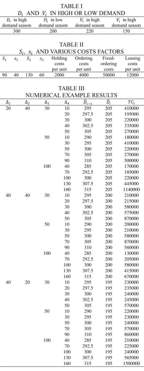
[image:4.595.306.550.48.192.2]

The calculation for the numerical analysis uses Matlab R2014b; the 500th _{period is used as a reference for analyzing.} Data assumptions for 𝐷𝑖 , 𝑉𝑖 , 𝑆𝑖 , 𝑠𝑖 and various costs factors (holding costs per unit, ordering cost per unit, fixed-ordering costs and leasing costs) in the off-peak season are made in TABLE I and TABLE II; while TABLE III does sensitivity analysis for changes in ∆.

TABLE I

𝐷𝑖 AND 𝑉𝑖 IN HIGH OR LOW DEMAND 𝐷𝑖 in high

demand season demand season 𝐷𝑖 in low demand season 𝑉𝑖 in high demand season 𝑉𝑖 in high

[image:4.595.49.290.154.772.2]

300 200 220 150

TABLE II

𝑆𝑖, 𝑠𝑖 AND VARIOUS COSTS FACTORS 𝑆1 𝑠1 𝑆2 𝑠2 Holding

costs per unit Ordering costs per unit Fixed-ordering costs Leasing costs per unit

90 40 130 60 2000 4000 50000 12000

TABLE III

NUMERICAL EXAMPLE RESULTS

∆1 ∆2 ∆3 ∆4 𝐷̃𝑖−1 𝐷̃𝑖 𝑇𝐶𝑖

20 40 30 10 295 205 410000

20 297.5 205 195000

30 40 50 300 302.5 305 205 205 205 220000 335000 270000

50 10

30 290 295 205 205 180000 410000

50 300 205 220000

70 90 305 310 205 205 270000 500000

100 40

70 285 292.5 205 205 170000 185000

100 300 205 220000

130 160 307.5 315 205 205 445000 1140000

40 40 30 10

20 295 297.5 200 200 210000 215000

30 300 200 580000

40 50 302.5 305 200 200 575000 870000

50 10

30 290 295 200 200 200000 210000

50 300 200 580000

70 90 305 310 200 200 870000 560000

100 40

70 285 292.5 200 200 130000 205000

100 300 200 580000

130 160 307.5 315 200 200 415000 670000

40 20 30 10

20 295 297.5 195 195 230000 235000

30 300 195 240000

40 50 302.5 305 195 195 245000 570000

50 10

30 290 295 195 195 220000 230000

50 300 195 240000

70 90 305 310 195 195 570000 860000

100 40

70 285 292.5 195 195 210000 225000

100 300 195 240000

130 160 307.5 315 195 195 565000 1500000

Fig.1. The effect on TC while ∆1> ∆2 and ∆4− ∆3 changed

(1) During the situation when ∆1> ∆2 and ∆3 are unchangeable, the larger ∆4 gets, TC will increase as well. (2) TC normally increases obviously while the difference between ∆3 and ∆4 increase.

(3) According to the numerical result, the minimum of TC can be obtained while ∆1= ∆2 and ∆4− ∆3= −60.

IV. CONCLUSION

Cost control is one of the problems that cannot be ignored in the maritime industry. With the development of the maritime market, the mastery of demand has become the key to controlling costs. By assuming the demand quantity as a triangular fuzzy number, the decision makers can consider the actual situation and set the upper and lower limits of the demand during different periods; which allow to predict the inventory quantity and the total cost more accurately in the estimation model.

By using Matlab in calculating numerical analysis results, while the larger ∆4 gets, the total cost will increase substantially, which means that the enterprise should guard against a sudden large amount of demand; otherwise, it will cause huge losses. In order to make the model more suitable to the realistic environment, hopefully this model is able to add more conditions in consideration in the future.

REFERENCES

[1] G. O. Young, “Synthetic structure of industrial plastics (Book style with paper title and editor),” in Plastics, 2nd ed. vol. 3, J. Peters, Ed. New York: McGraw-Hill, 1964, pp. 15–64.

[2] Ata Allah Taleizadeh, Seyed Taghi Akhavan Niaki, Mir-Bahador Aryanezhad, Nima Shafii, “A hybrid method of fuzzy simulation and genetic algorithm to optimize constrained inventory control systems with stochastic replenishments and fuzzy demand,” Information Sciences 220 (2013) 425–441

[3] Seyed Mohsen Mousavi, Seyed Taghi Akhavan Niaki, “Capacitated location allocation problem with stochastic location and fuzzy demand: A hybrid algorithm,” Applied Mathematical Modelling 37 (2013) 5109–5119

[4] Yuanji Xu, Jinsong Hu, “Random Fuzzy Demand Newsboy Problem,” SciVerse ScienceDirect, Physics Procedia 25 (2012) 924-931, 2012 Published by Elsevier B.V. Selection and/or peer-review under responsibility of Garry Lee

[5] Min Huang, Min Song, V. Jorge Leon and Xingwei Wang, “Decentralized capacity allocation of a single-facility with fuzzy demand,” Journal of Manufacturing Systems 33 (2014) 7– 15 [6] Feyzan Arikan, “A Two-Phased Additive Approach for Multiple

Objective Supplier Selection with Fuzzy Demand Level,” J. of Mult.-Valued Logic & Soft Computing, Vol. 22, pp. 373–385

[7] S. Sarkar* & T. Chakrabarti, “An EPQ Model of Exponential

210000 225000 240000

565000 1500000 0 200000 400000 600000 800000 1000000 1200000 1400000 1600000

-60 -30 0 30 60

To

ta

l Cos

t

International Journal of Industrial Engineering & Production Research, December 2013, Volume 24, Number 4 pp. 307-315

[8] Shengju Sang, “Coordinating a Three Stage Supply Chain with Fuzzy Demand,” Engineering Letters, 22:3 2014, ISSN: 1816-093X (Print); 1816-0948 (Online)

[9] Jianhua Yang, Zhichao Ma and Yang Song, “Research on the Support Model of Large Equipment Emergency Spare Parts under Fuzzy Demand,” Journal of Industrial Engineering and Management, JIEM, 2015 – 8(3): 658-673 – Online ISSN: 0953 – Print ISSN: 2013-8423

[10] M.F. Yang, M.C. Lo, and W.H. Chen, Member, IAENG, “Optimal Strategy for the Three-echelon Inventory System with Defective Product, Rework and Fuzzy Demand under Credit Period,” Engineering Letters, 23:4, 2015, ISSN: 1816-093X (Print); 1816-0948 (Online)

[11] Y. Long, L. H. Lee, E. P. Chew, Y. Luo, J. Shao, A. Senguta, S. M. L. Chua, “OPERATION PLANNING FOR MARITIME EMPTY CONTAINER REPOSITIONING,” International Journal of Industrial Engineering, 20(1-2), 141-152, 2013

[12] Rafael Diaz, Wayne Talley, Mandar Tulpule, “Forecasting Empty Containers Volumes,” The Asia Journal of Shipping and Logistics, Volumes 27 Number 2 August 2011 pp. 217-236

[13] Vineet Mittal, Dega Nagaraju and S. Narayanan, “Optimality Of Inventory Decisions In A Joint Two-Echelon Inventory System With And Without Fuzzy Demand,” International Journal of Applied Engineering Research, ISSN 0973-4562 Volume 10, Number 2 (2015) pp. 4497-4510

[14] I. Burhan Turksen, Tahir Khaniyev, and Fikri Gokpinar, “Investigation of fuzzy inventory model of type (s, S) with Nakagami distributed demands,” Journal of Intelligent & Fuzzy Systems 29 (2015) 531–538, DOI:10.3233/IFS-141309, IOS Press

[15] Wasim Akram Mandal and Sahidul Islam, “Fuzzy Inventory Model for Deteriorating Items, with Time Depended Demand, Shortages, and Fully Backlogging,” Pak.j.stat.oper.res. Vol. XII No.1 2016 pp101-109 [16] P. Parvathi and D. Chitra, “A Fuzzy Inventory Model for Vendor– Buyer Coordination in a Two Stage Supply Chain with Allowed Shortages,” International Journal of Computer Applications (0975 – 8887), Volume 76– No.2, August 2013

[17] M.F. Yang, M.C. Lo and W.H. Chen, “Optimal Strategy for the Three-echelon Inventory System with Defective Product, Rework and Fuzzy Demand under Credit Period,” Engineering Letters, Vol.23(2015), No.4,312-317. (EI)

[18] M.F. Yang, H.J. Tu and M.C. Lo, “A two-echelon inventory model for fuzzy demand with mutual beneficial pricing approach in a supply chain,” African Journal of Business Management (Accepted August 31, 2010). (Impact Factor 1.105, 58/112) (SSCI).

[19] M.F. Yang, M.J. Luo, C.Y. Shen, “Applying fuzzy theory to the