Polynomial Penalty Method for Solving Linear Programming Problems

(1)

Polynomial Penalty Method for Solving Linear

Programming Problems

Parwadi Moengin, Member, IAENG

Abstract—In this work, we study a class of polynomial order-even penalty functions for solving linear programming problems with the essential property that each member is convex polynomial order-even when viewed as a function of the multiplier. Under certain assumption on the parameters of the penalty function, we give a rule for choosing the parameters of the penalty function. We also give an algorithm for solving this problem.

Index Terms—linear programming, penalty method, polynomial order-even.

I.INTRODUCTION

The basic idea in penalty method is to eliminate some or all of the constraints and add to the objective function a penalty term which prescribes a high cost to infeasible points (Wright, 2001; Zboo, etc., 1999). Associated with this method is a parameter σ, which determines the severity of the penalty and as a consequence the extent to which the resulting unconstrained problem approximates the original problem (Kas, etc., 1999; Parwadi, etc., 2002). In this paper, we restrict attention to the polynomial order-even penalty function. Other penalty functions will appear elsewhere. This paper is concerned with the study of the polynomial penalty function methods for solving linear programming. It presents some background of the methods for the problem. The paper also describes the theorems and algorithms for the methods. At the end of the paper we give some conclusions and comments to the methods.

II.STATEMENT OF THE PROBLEM

Throughout this paper we consider the problem minimize ்ܿݔ

subject to Ax = b

x ≥ 0, (1)

where A ∈

R

m×n, c, x ∈

R

n, and b ∈

R

m. Without loss of generality we assume that A has full rank m. We assume that problem (1) has at least one feasible solution. In order to solve this problem, we can use Karmarkar’s algorithm and simpelx method (Durazzi, 2000). But in this paper we propose a polynomial penalty method as another alternative method to solve linear programming problem (1).

Manuscript is submitted on March 6, 2010. This work was supported by the Faculty of Industrial Engineering, Trisakti University, Jakarta.

Parwadi Moengin is with the Department of Industrial Engineering, Faculty of Industrial Technology, Trisakti University, Jakarta 11440, Indonesia. (email: parwadi@hotmail.com, parwadi@trisakti.ac.id).

III. POLYNOMIAL PENALTY METHOD

For any scalar σ > 0, we define the polynomial penalty function

P

(

x

,

σ

)

for problem (1);

P

(

x

,

σ

)

:

R

n

→

by

)

,

(

x

σ

P

=

c

T

x

+

∑

=

ρ

−

σ

m

i i i

b

x

A

1

)

(

, (2)

where ρ > 0 is an even number. Here,

A

_i and

b

_i denote the ith row of matrices A and b, respectively. The positive even number ρ is chosen to ensure that the function (2) is convex. Hence,

P

(

x

,

σ

)

has a global minimum. We refer to σ as the penalty parameter.

This is the ordinary Lagrangian function in which in the altered problem, the constraints

A

_i

x

−

b

_i (i =1,..,m)

are replaced by

(

A

i

x

−

b

i

)

ρ. The penalty terms are formed from a sum of polynomial order−ρ of constrained violations and the penalty parameter σ determines the amount of the penalty.

The motivation behind the introduction of the polynomial order-ρ term is that they may lead to a representation of an optimal solution of problem (1) in terms of a local unconstrained minimum. Simply stating the definition (2) does not give an adequate impression of the dramatic effects of the imposed penalty. In order to understand the function stated by (2) we give an example with some values for σ. Some graphs of

P

(

x

,

σ

)

are given in Figures 1−3 for the trivial problem

minimize

f

(

x

)

=

x

subject to

x

−

1

=

0

,

for which the polynomial penalty function is given by

)

,

(

x

σ

P

=

x

+

σ

(

x

−

1

)

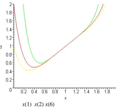
ρ.

Figures 1, 2 and 3 depict the one-dimensional variation of the penalty function of ρ = 2, 4 and 6, for three values of penalty parameter σ, that is σ = 1, σ = 2 and σ = 6, respectively.

(2)

[image:2.612.68.290.51.667.2]

x(1) x(2) x(6)

Figure 1 The quadratic penalty function for ρ = 2

[image:2.612.75.282.58.244.2]

x(1) x(2) x(6)

Figure 2 The polynomial penalty function for ρ = 4

x(1) x(2) x(6)

Figure 3 The polynomial penalty function for ρ = 6

The y-ordinates of these figures represent

P

(

x

,

σ

)

for ρ = 2, ρ = 4, ρ = 6, respectively. Clearly, if the solution x * = 1 of this example is compared with the points which

minimize

P

(

x

,

σ

)

, it is clear that x * is a limit point of the unconstrained minimizers of

P

(

x

,

σ

)

as σ → ∞.

The intuitive motivation for the penalty method is that we seek unconstrained minimizers of

P

(

x

,

σ

)

for value of σ increasing to infinity. Thus the method of solving a sequence of minimization problem can be considered.

The polynomial penalty method for problem (1) consists of solving a sequence of problems of the form

minimize

P

(

x

,

σ

k

)

subject to

x

≥

0

, (3)

where

{ }

σ

k is a penalty parameter sequence satisfying

1

0

<

σ

k

<

σ

k+

for all k,

σ

k

→

∞

.

The method depends for its success on sequentially increasing the penalty parameter to infinity. In this paper, we concentrate on the effect of the penalty parameter.

The rationale for the penalty method is based on the

fact that when

σ

k

→

∞

, then the term

∑

=

ρ

−

σ

m

i

i i k

A

x

b

1

)

(

,

when added to the objective function, tends to infinity if

0

≠

−

_i i

x

b

A

and equals zero if

A

_i

x

−

b

_i

=

0

for all i. Thus, we define the function

]

,

(

:

R

n

→

−∞

+

∞

f

by

⎩

⎨

⎧

≠

−

∞

=

−

=

.

all

for

0

if

,

all

for

0

if

)

(

i

b

x

A

i

b

x

A

x

c

x

f

i i

i i T

The optimal value of the original problem (1) can be written as

f * =

c

T

x

x b

Ax

inf

= , ≥0 =

inf

x≥0

f

(

x

)

=

)

,

(

lim

inf

k

x≥0 →∞

P

x

σ

. (4) On the other hand, the penalty method determines, via the

sequence of minimizations (3),

)

,

(

inf

lim

k

x

k

P

x

f

=

σ

≥ ∞

→ 0 . (5)

Thus, in order for the penalty method to be successful, the original problem should be such that the interchange of “lim” and “inf” in (4) and (5) is valid. Before we give a guarantee for the validity of the interchange, we investigate some properties of the function defined in (2).

First, we derive the convexity behavior of the polynomial penalty function defined by (2) is stated in the following stated theorem.

Theorem 1 (Convexity)

The polynomial penalty function

P

(

x

,

σ

)

is convex in its domain for every σ > 0. [image:2.612.83.272.484.657.2]

(3)

Proof.

It is straightforward to prove convexity of

P

(

x

,

σ

)

using the convexity of

c

T

x

and

(

A

_i

x

−

b

_i

)

ρ. Then the theorem is proven.

The local and global behavior of the polynomial penalty function defined by (2) is stated in next the theorem. It is a consequence of Theorem 1.

Theorem 2 (Local and global behavior)

Consider the function

P

(

x

,

σ

)

which is defined in (2). Then

(a)

P

(

x

,

σ

)

has a finite unconstrained minimizer in its domain for every σ > 0 and the set Mσ of unconstrained minimizers of

P

(

x

,

σ

)

inits domain is convex and compact foreveryσ > 0.

(b) Any unconstrained local minimizer of

P

(

x

,

σ

)

in its domain is also a global unconstrained minimizer of

P

(

x

,

σ

)

.

Proof.

It follows from Theorem 1 that the smooth function

)

,

(

x

σ

P

achieves its minimum in its domain. We then conclude that

P

(

x

,

σ

)

has at least one finite unconstrained minimizer.

By Theorem 1

P

(

x

,

σ

)

is convex, so any local minimizer is also a global minimizer. Thus, the set Mσof unconstrained minimizers of

P

(

x

,

σ

)

is bounded and closed, because the minimum value of

P

(

x

,

σ

)

is unique, and it follows that Mσis compact. Clearly, the convexity of Mσ follows from the fact that the set of optimal points

P

(

x

,

σ

)

is convex. Theorem 2 has been verified.

As a consequence of Theorem 2 we derive the monotonicity behaviors of the objective function problem (1), the penalty terms in

P

(

x

,

σ

)

and the minimum value of the polynomial penalty function

P

(

x

,

σ

)

. To do this, for any

σ

k > 0 we denote

x

k and

P

(

x

k

,

σ

k

)

as a minimizer and minimum value of problem (3),

respectively.

Theorem 3 (Monotonicity)

Let

{

σ

k

}

be an increasing sequence of positive penalty parameters such that

σ

k

→

∞

as

k

→

∞

.

Then

(a)

{

c

T

x

k

}

is non-decreasing.

(b)

⎭

⎬

⎫

⎩

⎨

⎧

∑

−

= ρ m i i k i

x

b

A

1

)

(

is non-increasing.

(c)

{

P

(

x

k

,

σ

k

)

}

is non-decreasing.

Proof.

Let

x

k and

x

k+1 denote the global minimizers of

problem (3) for the penalty parameters

σ

k and

σ

k+1,

respectively. By definition of

x

k and

x

k+1 as

minimizers and

σ

k <

σ

k+1, we have

k k T

x

c

+

σ

∑

= ρ

−

m i i k i

x

b

A

1

)

(

≤

c

T

x

k+1

+ k

σ

∑

= ρ +

−

m i i k i

x

b

A

1

)

(

, (6a)

1

+ k T

x

c

+

σ

k

∑

= ρ +

−

m i i k i

x

b

A

1 1

)

(

≤ 1 + k T

x

c

+

σk +1

∑

= ρ +

−

m i i k i

x

b

A

1

)

(

, (6b)

1

+ k T

x

c

+ σk +1

∑

= ρ +

−

m i i k i

x

b

A

1 1

)

(

≤ k T

x

c

+

σk +1

∑

= ρ

−

m i i k i

x

b

A

1

)

(

. (6c)

We multiply the first inequality (6a) with the ratio

σ

k+1/ k

σ

, and add the inequality to the inequality (6c) we obtain

1 1

1

+ +

+

⎟⎟

⎠

⎞

⎜⎜

⎝

⎛

−

σ

≤

⎟⎟

⎠

⎞

⎜⎜

⎝

⎛

−

σ

T k

k k k T k k

x

c

x

c

.

Since 0 <

σ

k _<

σ

k+1

, it follows that

c

T

x

k

≤

c

T

x

k+1 and part (a) is established.

To prove part (b) of the theorem, we add the inequality (6a) to the inequality (6c) to get

(

)

∑

(

)

∑

= ρ + = ρ +

+ ₋_σ ₋ _≤ _σ ₋_σ ₋

σ m i i k i k k m i i k i k

k _A_x _b _A_x _b

1 1

1 ₍ ₎ ₍ ₎

, thus

∑

= ρ = ρ

+

−

≤

m

−

i i k i m i i k

i

x

b

A

x

b

A

1 1

1

)

(

)

(

as required for part (b).

Using inequalities (6a) and (6b), we obtain

k k T

x

c

+

σ

∑

= ρ

−

m i i k i

x

b

A

1

)

(

≤

c

T

x

k+1_{+ σ}k +1

∑

= ρ +

−

m i i k i

x

b

A

1

)

(

.

Hence, part (c) of the theorem is established.

We now give the main theorem concerning polynomial penalty method for linear programming problem (1).

(4)

Theorem 4 (Convergence of polynomial penalty function)

Let

{

σ

k

}

be an increasing sequence of positive penalty parameters such that

σ

k

→

∞

as

k

→

∞

. Denote

k

x

and

P

(

x

k

,

σ

k

)

as in Theorem 3. Then (a)

Ax

k

→

b

as

k

→

∞

.

(b)

c

T

x

k

→

f

*

as

k

→

∞

. (c)

P

(

x

k

,

σ

k

)

→

f

*

as

k

→

∞

.

Proof.

By definition of

x

k and

P

(

x

k

,

σ

k

)

, we have k

T

x

c

≤

P

(

x

k

,

σ

k

)

_≤

P

(

x

,

σ

k

)

for all

x

≥

0

. (7)

Let f * denotes the optimal value of the problem

(

P

)

. We have

f * =

c

T

x

x b

Ax

inf

= , ≥0 =

inf

(

,

)

k

xAx b

x

P

σ

≥0=

.

Hence, by taking the infimum of the right-hand side of (7) over

x

≥

0

and

Ax

=

b

, we obtain

)

,

(

x

k k

P

σ

=

c

T

x

k +

σ

k

∑

=

ρ

−

m

i

i k i

x

b

A

1

)

(

≤ f *.

Let

x

be a limit point of

{

x

k

}

. By taking the limit superior in the above relation and by using the continuity

of

c

T

x

and

A

_i

x

−

b

_i, we obtain

x

c

T

+

∑

=

ρ ∞

→

σ

−

m

i

i k i k

k

sup

₁

(

A

x

b

)

lim

≤ f *. (8)

Since

∑

=

ρ

−

m

i

i k i

x

b

A

1

)

(

≥ 0 and

σ

k

→

∞

, it follows

that we must have

∑

=

ρ

−

m

i

i k i

x

b

A

1

)

(

→

0

and

0

=

−

_i i

x

b

A

for all i = 1, …, m, 9) otherwise the limit superior in the left-hand side of (8)

will equal to +∞. This proves part (a) of the theorem.

Since

{

x

∈

R

n

x

≥

0

}

is a closed set we also obtain

that

x

≥

0

. Hence,

x

is feasible, and

f * ≤

c

T

x

. (10) Using (8)-(10), we obtain

f * +

∑

=

ρ ∞

→

σ

−

m

i

i k i k

k

sup

₁

(

A

x

b

)

lim

≤

c

T

x

+

∑

=

ρ ∞

→

σ

−

m

i

i k i k k

b

x

A

1

)

(

sup

lim

≤ f *.

Hence,

∑

=

ρ ∞

→

σ

−

m

i

i k i k

k

A

x

b

1

)

(

sup

lim

= 0

and

f * =

c

T

x

,

which proves that

x

is a global minimum for problem (1). This proves part (b) of the theorem.

To prove part (c), we apply the results of parts (a) and (b),

and then taking

k

→

∞

of the definition

P

(

x

k

,

σ

k

)

.

Some notes about this theorem will be taken. First, it assumes that the problem (3) has a global minimum. This may not be true if the objective function of the problem (1) is replaced by a nonlinear function. However, this situation may be handled by choosing appropriate value of ρ. We also note that the constraint

x

≥

0

of the problem (3) is important to ensure that the limit point of

the sequence

{

x

k

}

satisfies the condition

x

≥

0

.

IV. ALGORITHM

The implications of these theorems are remarkably strong. The polynomial penalty function has a finite unconstrained minimizer for every value of the penalty parameter, and every limit point of a minimizing sequence for the penalty function is a constrained minimizer of a problem (1). Thus the algorithm of solving a sequence of minimization problems is suggested. Based on Theorems 4, we formulate an algorithm for solving problem (1).

Algorithm 1

Given Ax = b,

σ

1 > 0, the number of iteration N and ε

> 0.

1. Choose

x

1 ∈

R

nsuch that A

x

1 = b and

x

1 ≥ 0. 2. If the optimality conditions are satisfied for problem

(1) at

x

1, then stop.

3. Compute

P

(

x

1

,

σ

1

)

:=

min

(

,

1

)

0

σ

≥

P

x

x and the

minimizer

x

1.

4. Compute

P

(

x

k

,

σ

k

)

:=

min

(

,

)

0

k

x

P

x≥

σ

, the

minimizer

x

k and

σ

k := 10

σ

k−1 for k = 2.

5. If ||

x

k

−

x

k−1|| < ε or |

P

(

x

k

,

σ

k

)

–

)

,

(

x

k−1

σ

k−1

P

| < ε or ||

Ax

k

−

b

_{|| < ε or}

k = N; then stop. Else k := k + 1 and go to step 4.

(5)

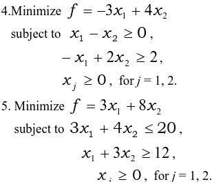
Examples: Consider the following problems. 1.Minimize

f

=

2

x

₁

+

5

x

₂

+

7

x

₃

subject to

x

₁

+

2

x

₂

+

3

x

₃

=

6

,

x

_j

≥

0

, for j = 1, 2, 3. 2.Minimize

f

=

0

.

4

x

₁

+

0

.

5

x

₂ subject to

0

.

3

x

₁

+

0

.

1

x

₂

≥

2

.

7

,

0

.

5

x

₁

+

0

.

5

x

₂

=

6

,

x

_j

≥

0

, for j = 1, 2. 3.Minimize

f

=

4

x

₁

+

3

x

₂

subject to

2

x

₁

+

3

x

₂

≥

6

,

4

x

₁

+

x

₂

≥

4

,

x

_j

≥

0

, for j = 1, 2.

4.Minimize

f

=

−

3

x

₁

+

4

x

₂

subject to

x

₁

−

x

₂

≥

0

,

−

x

₁

+

2

x

₂

≥

2

,

x

j

≥

0

, for j = 1, 2. 5. Minimize

f

=

3

x

₁

+

8

x

₂

subject to

3

x

₁

+

4

x

₂

≤

20

,

x

₁

+

3

x

₂

≥

12

,

0

≥

j [image:5.612.63.513.38.423.2]

x

, for j = 1, 2.

Table 1 reports the results of computational for Algorithm 1(ρ = 2), Algorithm 1(ρ = 4) and Karmarkar’s Algorithm. The first column of Table 1 contains the problem number and the next two columns of each algorithm in this table contain the total iterations and the times (in seconds) of each algorithm.

Tabel 1 Algorithm 1(ρ = 2), Algorithm 1(ρ = 4) and Karmarkar’s Algorithm test statistics

Problem No.

Algorithm 1(ρ = 2) Algorithm 1(ρ = 4) Karmarkar’s Algorithm

Total Iterations

Time (Secs.)

Total Iterations

Time (Secs.)

Total Iterations

Time (Secs.) 1.

2. 3. 4. 5.

10 9 9 10 10

3.4 3.9 8.5 8.7 9.9

25 7 9 12 19

189.1 75.3 851.4 2978.9 5441.7

16 19 19 12 18

3.6 3.7 3.7 2.8 3.8

V. CONCLUSION

As mentioned above, the paper has described the penalty functions with penalty terms in polynomial order-σ for solving problem (1). The algorithms for these methods are also given in this paper. The Algorithm 1 is used to solve the problem (1). We also note the important thing of these methods which do not need an interior point assumption.

REFERENCES

[1] Durazzi, C. (2000). On the Newton interior-point method for nonlinear programming problems. Journal of Optimization Theory and Applications. 104(1). pp. 73−90.

[2] Kas, P., Klafszky, E., & Malyusz, L. (1999).Convex program based on the Young inequality and its relation to linear programming. Central European Journal for Operations Research. 7(3). pp. 291−304.

[3] Parwadi, M., Mohd, I.B., & Ibrahim, N.A. (2002). Solving Bounded LP Problems using Modified Logarithmic-exponential Functions. In Purwanto (Ed.), Proceedings of the National Conference on Mathematics and Its Applications in UM Malang (pp. 135-141). Malang: Department of Mathematics UM Malang.

[4] Wright, S.J. (2001). On the convergence of the Newton/log-barrier method. Mathematical Programming, 90(1), 71−100.

[5] Zboo, R.A, Yadav, S.P., & Mohan, C. (1999).Penalty method for an optimal control problem with equality and inequality constraints. Indian Journal of Pure and Applied Mathematics. 30(1), pp. 1−14.

[image:5.612.322.476.48.180.2]